國 立 交 通 大
學
管 理 科 學 研 究 所
碩 士 論 文
為何股票能在高系統性風險事件下優於大盤
─ 企業成長策略之觀點
Why the Stocks Can Outperform the Market Following the
Black Events:
From the Perspective of the Growth Strategy
研 究 生:王瓊萱
指導教授:王淑芬 博士
包曉天 博士
為何股票能在高系統性風險事件下優於大盤
─ 企業成長策略之觀點
Why the Stocks Can Outperform the Market Following the Black Events:
From the Perspective of the Growth Strategy
研 究 生:王瓊萱 Student:Wang, Chiung-Hsuan
指導教授:王淑芬 博士 Advisor:
包曉天 博士
國 立 交 通 大 學
管理科學研究所
碩 士 論 文
A ThesisSubmitted to Department of Management Science College of Management
National Chiao Tung University in partial Fulfillment of the Requirements for the Degree of Master in Management Science
June 2012
Hsinchu, Taiwan, Republic of China
中 華 民 國 一百零一 年 六 月
Dr. Wang, Sue-Fung
Dr. Bao, Xiao-Tian
i
為何股票能在高系統性風險事件下優於大盤 ─ 企業成長策略之觀點
研究生:王瓊萱 指導教授:王淑芬 博士
包曉天 博士
國立交通大學管理科學研究所碩士班
摘要
過去文獻指出,公司成長策略與市場評價之間抱持兩種相反的假說:
「資訊不對稱假說」以及「綜效理論」。雖然這些文獻比較多角化公司與
聚焦化公司差異,但卻無法得到決定性的一致結論。本研究觀察在高系統
風險事件下,比較兩種成長策略的差異,以及一間企業的多角化程度與市
場評價之間的關係。結果一致性的支持「資訊不對稱假說」,顯示多角化
公司的市場評價較低;企業多角化程度越高,市場給予的評價越低。此外,
本研究更進一步去觀察發生高系統風險事件後,企業多角化程度的改變與
市場評價,發現多角化程度增加之公司相較於未改變之公司得到較差的市
場評價。最後,本研究使用不同的多角化衡量方法使得研究具穩健性,並
且結論一致性的支持「資訊不對稱假說」。
關鍵字:成長策略、多角化、市場評價、黑色事件
33
Why the Stocks Can Outperform the Market Following the Black Events:
─ From the Perspective of the Growth Strategy
Student:Wang, Chiung-Hsuan Advisor:Dr. Wang, Sue-Fung,
Dr. Bao, Xiao-Tian
Graduate Institute of Management Science
National Chiao Tung University
Abstract
According to previous studies, two competing arguments exist in explaining the relation between diversification and the market value, namely, the “information asymmetry hypothesis” and the “theory of synergy”. Although there is a substantial literature that compares diversified firms to focused firms, this literature has not reached a decisive conclusion. In this paper, we investigate whether the market's valuation of a firm is correlated with its degree of diversification following the “black events”. The results are consistent with the “information asymmetry hypothesis”, and show significantly negative relation between the degree of corporate diversification and Tobin’s Q, even after controlling for other determinants. We show further that diversified firms have lower Q's and BHARs than equivalent portfolios of focused firms. And firms that increase their number of segments have significantly lower Q's than firms that keep their number of segment constant after the black event happened. Overall, our main findings are robust to various measures in diversification, and our evidence is consistent with the “information asymmetry hypothesis”
iii
誌 謝
本論文得以順利完成,首先要感謝指導教授王淑芬老師以及包曉天老師
這一年多來的建議與教導。於學術研究與論文撰寫方面,王老師往往付出
更多的時間讓我們的問題能得到最完整的解答,為我們訂正論文疏漏之處,
耐心指導學生論文研究方向與撰寫,真的很感謝王老師孜孜不倦的指導並
且提供豐富的資源,讓我的論文能順利的完成並且也開拓學生的理論與實
務上的視野,我將一輩子銘記在心。此外,感謝口試委員葉銀華、施懿宸
以及王衍智抽空仔細閱讀本論文、參與口試,提供寶貴的意見,給我的建
議與肯定,讓我把論文寫的更臻完善。
同時,也十分感謝陪我一路走過風風雨雨的王家同伴們,給我寶貴的建
議和鼓勵。另外也要感謝我們碩班的同學們,在兩年的學習過程,彼此關
心、打氣,一起討論作業、學習與成長。祝福大家鵬程萬里、身體健康。
最後,我要感謝我的父母親以及我可愛的妹妹。不論我遭遇任何挫折都在
我身邊給予我鼓勵與支持,家人的鼓勵是我勇於挑戰的原動力,有家人的
支持才使我更加堅強。我願把這份榮耀和各位分享,謝謝!
iv
目 錄
中文摘要 ... i 英文摘要 ... ii 誌 謝 ... iii 目 錄 ... iv 圖 目 錄 ... vi 1. Introduction ... 1 2. Methodology ... 8 2.1. Data Source ... 82.2. Long-Run Stock Performance Following the Black Events ... 9
2.2.1. Buy-and-Hold Abnormal Returns (BHARs) ... 10
2.3. Definition of variables ... 12
2.3.1. Growth Strategy ─ the measurements of diversification ... 12
2.3.2. Tobin’s Q ... 13
2.3.3.Other Control Variables ... 14
3. Empirical Results ... 16
3.1 Descriptive Statistics ... 16
3.2 t-test for mean of two subsamples. ... 17
3.3 Correlation Matrix ... 19
3.4 Cross-sectional Regression Analysis ... 20
3.5 Regression s of Q and three measurements of diversification and controls. ... 23
3.6 Literature Review ─ Adjusted ... 24
3.7 Q and change in the degree of diversification following the black event ... 25
4. Conclusion ... 26
References ... 28
v
表 目 錄
Table 1 Number and percentage of company in each industry among three main stock
exchanges ... 9
Table 2 BHAR Adjusted by CRSP Nasdaq Value-Weighted Market Return ... 11
Table 3 Sample Distribution by Industry Type and Growth Strategy ... 12
Table 4 Descriptive Statistics ... 17
Table 5 t-test for mean of two subsamples ... 18
Table 6 Correlation matrix ... 20
Table 7 Cross-sectional Regressions of Q and three measurements of diversification and controls ... 22
Table 8 Regression s of Q and three measurements of diversification and controls ... 24
Table 9 Adjusted ... 25
Table 10 t-test for mean of Q ... 26
vi
圖 目 錄
1
1. Introduction
Market efficiency hypothesis argues that markets are rational and the prices fully reflect all available information. Due to the timely actions of investors prices of stocks quickly adjust to the new information, and reflect all the available information; therefore, no investor can beat the market by generating abnormal returns. However, it is found in many stock exchanges of the world that these markets are not following the rules of EMH. The functioning of these stock markets deviate from the rules of EMH, and thus deviations are called anomalies. According to George & Elton (2001), anomalies are defined as irregularity or a deviation from common or natural order or an exceptional condition. While in standard finance theory, financial market anomaly means a situation in which a performance of stock or a group of stocks deviate from the assumptions of efficient market hypotheses. Such movements or events which cannot be explained by using efficient market hypothesis are called financial market anomalies.
There are a lot of researches done on the existence of various types of anomalies. From the perspective of the market environment, we can find that some investors can beat the market and generate abnormal returns. Different authors segregated anomalies into three main types: calendar anomalies, fundamental anomalies and technical anomalies. Calendar anomalies exist due to deviation in normal behaviors of stocks with respect to time periods, including weekly effect, January effect, and Turn-of-the-Month Effect. Another type is fundamental anomalies that prices of stocks are not fully reflecting their intrinsic values, including dividend yield anomaly, price to earnings ratio anomaly and low price to book anomaly. Technical anomalies are based upon the past prices and trends of stocks; for example, momentum effect.
2
Technical anomalies also include trading strategies like moving averages and trading breaks which includes resistance and support level ( Madiha Latif, Shanza Arshad, Mariam Fatima, and Samia Farooq, 2011 ).
Form the prospect of business operations, there are also many studies done on anomalies; for instance, size effect and corporate governance. In terms of size and market valuation, size effect, which is the most prevalent theory proposed by Fama and French (1992), argues that investors demand higher return due to the higher risks of smaller firms. However, the theory is still subject to counter arguments and debates. Fernandes and Ferreira (2007) find a significantly negative relation between size and Tobin’s Q (hereafter, Q), whereas Moses (1987) proves that size and Q are positively correlated. Thus, both directions between size and market valuation are possible. As for corporate governance, Sanjai Bhagat and Brian Bolton (2008) found that better governance is significantly positively correlated with better contemporaneous and subsequent operating performance.
Ansoff (1957) first used the term “diversification” to illustrate corporate growth strategies. And the most researched linkage in the strategic management literature is that involving diversification and performance ( Leslie E. Palich, Laura B. Cardinal, and C. Chet Miller, 2000; Sheng-Syan Chen, 2006). Growth strategies (i.e., organizational form), focus versus diversification, become more and more important since these growth strategies play a vital role in explaining the valuation effects on firms. A number of studies have carefully investigated how growth strategy exerts an effect on Q (e.g., Bhagat, Shleifer, and Vishny, 1990; Berger and Ofek, 1996; Servaes, 1996; and Heron and Lie, 2002).
3
Diversification is defined both narrowly and broadly. As Villalonga (2004) points out, SFAS 141 defines a segment as “a component of an enterprise engaged in providing a product or service or a group of related product and services primarily to unaffiliated customers for a profit.” Furthermore, Ramanujam and Varadarajan (1989) define diversification as “the entry of a firm or business unit into new lines of activity, either by process of internal business development or acquisition, which entails changes in its administrative structure, system, and other management processes.” Lim, Thong, and Ding (2008) use three methods to measure the degree of diversification, namely, the number of segments in a corporation, Herfindahl index (HI) from sales, and diversification dummy. All these measurements are narrow definitions of diversification. In the current study, we selected all of the three narrow definitions to analyze the diversification of a company. Thus, we would like to clarify that in this work, “segment” is used instead of “subsidiary” for diversification.
Lang & Stulz (1994);Berger & Ofek (1995) explain the corporate diversification discount; they found that diversified firms trade at a discount relative to focused firms in the same industries. As mentioned by Wernerfelt and Montgomery (1998), Lang and Stulz (1994), Servaes (1996), Chen (2006), Chen (2008), and others, focused firms tend to exhibit better investment opportunities than diversified firms. The fundamental argument made against corporate diversification is that it somehow exacerbates managerial agency problems. Inefficient investments due to cross-subsidization between divisions can exist in diversified firms. Shin and Stulz (1998) and Rajan et al. (2000) find evidence of inefficient diversion of corporate resources from divisions with good investment opportunities to failing divisions. Therefore, agency problems have been proposed as an explanation for the
1
A formal document issued by the Financial Accounting Standards Board (FASB), which details accounting standards and guidance on selected accounting policies set out by the FASB. The standards are created to ensure a higher level of corporate transparency.
4
diversification discount effect, and the negative impacts of corporate diversification can be referred to the agency cost hypothesis. Also, managers frequently cite the desire to mitigate asymmetric information as a motivation for increasing firm focus (Jonathan E. Clarke, C. Edward Fee, and Shawn Thomas, 2004). Diversified firms are subject to larger asymmetric information problems than are focused firms, and diversified firms operate with less efficiency.
On the other hand, Villalonga (2004) uses new database (Business Information Tracking Series) and finds the diversification premium. Besides, the premium is robust to variation in the sample, business unit definition and measures of excess value and diversification. Indeed, the management in diversified firms can broaden their internal capital market and acquire these economies by diversifying. For instance, a diversified firm can bypass the external capital market by shifting funds from business segments with poorer investment opportunities to business segment with better investment opportunities. This suggests that diversified firms allocate resources more efficiently. Morck and Yeung (1998) propose the theory of synergy, indicating that the benefits of synergy come from the existence of valuable information-based assets within the firm. According to Thomas (2002), diversified firms have potential information benefits of diversification. Aggarwal and Samwick (2003) also report that the advantage of diversification outweighs its drawback.
As mentioned previously, Villalonga (2004) use a new database (Business Information Tracking Series) and finds the diversification premium which is robust to variation in the sample, business unit definition, and measures of excess value and diversification. According to Morck and Yeung (1998), the theory of synergy indicates that diversification contributes the value of market. However, earlier studies, such as Lang and Stulz (1994), find that Q and firm diversification are negatively
5
related because of diversification discount, that is, firms operate with less efficiency. Berger and Ofek (1995) claim that diversified firms trade at a discount relative to single-segment firms in the same industries. This phenomenon might be attributed to agency cost for outside investors due to information asymmetry. Therefore, the relation between diversification and market valuation is still inconclusive.
The 20th anniversary of what came to be known as “Black Monday”—19 October 1987—provides a memorable platform for considering, yet again, the role of risk in our financial markets (John C. Bogle, 2008). On that single day, the Dow Jones Industrial Average dropped from 2,246 to 1,738, an astonishing decline of almost 25 percent. In fact, during 2007, we witnessed an unprecedented series of amazing market swings, known as financial tsunami. Whereas in the 1990s and 2000s, the daily changes in the level of stock prices typically exceeded 5 percent only one time or two times a year. For example, the Asian financial crisis, internet bubble, Enron financial scandal, the September 11, 2001 terrorist attacks. In this paper, we call these events with rarity, extremeness, and retrospective predictability “Black Events”. Refer to “Black Monday,” the definition of “Black Events” is that the Dow Jones Average Index fell over 5% (greater than 5%) in one day. These stunning declines shocked nearly all market participants, although some veterans were not surprised, outperformed the market even. As a result, these big-shock events provided an opportunity to examine the role of growth strategy in explaining the benefit to the market valuation.
A number of studies discuss the relation between diversification and the firm value. Moreover, this study wants to see the difference of growth strategy in special condition, as called “Black Events”. This study contributes to the literature by examining the importance of focus versus diversification in explaining the value from
6
market following the black event. In a sample of 534 outperformed firms from 2002 to 2004, our findings indicate that long-run valuation effect (BHARs) of corporate growth strategy is differentiated. Our evidence leads to the conclusion that there is a negative relation between Q and diversification. The reason for this relation does not appear to be that good firms diversify and therefore become bad firms. In our sample, there is some evidence that multi-segment firms are firms with lower Q's relative to other focused firms but not relative to firms in their industry. This evidence could imply that firms diversify when they no longer have growth opportunities in their industry or that the market anticipates ill-fated diversification and already impounds it in the firm's value.
Our results are important for two specific reasons. At first, there has been no empirical evidence on the role of growth strategy in explaining the value from market following the black event. Furthermore, by taking into account the issue on the effect of focus and diversification on the value from market following the black event, this study also adds to existing literature on whether the nature of growth strategy is an important consideration in assessing the value from market. Our main findings are robust to different measures in diversification.
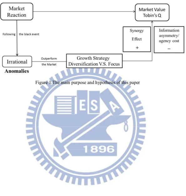
Figure 1 shows this paper’s background about the relationship between
diversification and market valuation. Apparently, both signs are possible for each study. Previous studies might point out either positive or negative relation between diversification and Q. However, such results might be biased or distorted due to the failure to consider other variable. Here, we use a broader perspective to examine the whole picture of diversification and market valuation.
The remainder of this paper is organized in sections. Section 2 explains the methodology, including the sample selection, variable definitions and model. Section
7
3 presents the empirical results and findings on the value from market. Finally, section 4 provides the summaries and conclusions.
8
2. Methodology
2.1. Data Source
This section describes the data sources that we use to conduct our study. As previous sections mention, there are several black events happened in these years. Financial scandals, like Enron, disclosure that the corporate managers engaged in earnings manipulation and accounting irregularities to inflate the stock price and gain from their equity and options holdings. Finally, in 2001, many of the corporate law reforms enacted in the United State have come as a response to corporate scandals. In the same time, terrorist attacked the United State and shocked the market. As a result, we collect an initial sample between January 2002 and December 2004. Stock prices from the original sample were collected from the Center for Research on Security Prices (CRSP).
The main stock exchanges in United State are NASDAQ, NYSE, and AMEX. NASDAQ has established itself as an indicator of the performance of stocks of technology companies and growth companies. The data collected from three individual stock exchange websites indicate that NASDAQ has the biggest percentage of technology firms (see Table 1). A previous study has shown that investors are periodically overoptimistic as regards the earnings potential of young growth companies (Loughran & Ritter, 1995). As a result, issuers can report unusually high earnings by adopting discretionary accounting accruals adjustments that raise reported earnings relative to actual cash flows (Teoh, Welch, & Wong, 1998). We speculate that the possibilities of these firms are higher. Therefore, it’s easier to see the relation between growth strategy and market value. Thus, the current study focuses on
9
NASDAQ, and data we use were collected from Compustat Industry Segment (CIS) database and Wharton Research Data Services (WRDS).
Table 1 Number and percentage of company in each industry among three main stock exchanges
Stock Exchange
NASDAQ NYSE AMEX ALL Statistic No. % No. % No. % No. % Basic Industries 78 2.77 191 5.89 74 14.02 343 5.21 Capital Goods 202 7.18 186 5.73 31 5.87 419 6.36 Consumer Durables 253 8.99 104 3.21 31 5.87 388 5.89 Consumer Non-Durables 124 4.40 122 3.76 22 4.17 268 4.07 Consumer Services 345 12.26 413 12.73 45 8.52 803 12.19 Energy 103 3.66 213 6.57 39 7.39 355 5.39 Finance 600 21.31 468 14.43 25 4.73 1,093 16.59 Health Care 232 8.24 88 2.71 30 5.68 350 5.31 Miscellaneous 87 3.09 47 1.45 4 0.76 138 2.10 Public Utilities 89 3.16 225 6.94 11 2.08 325 4.93 Technology 514 18.26 142 4.38 29 5.49 685 10.40 Transportation 57 2.02 59 1.82 0 0.00 116 1.76 N/A 131 4.65 986 30.39 187 35.42 1,304 19.80 TOTAL 2,815 100 3,244 100 528 100 6,587 100
2.2. Long-Run Stock Performance Following the Black Events
As mentioned by previous studies, measuring long-run stock returns remains heavily debated in the asset pricing literature (e.g., Barber and Lyon, 1997; Fama, 1998; Loughran and Ritter, 2000; and Michell and Stafford, 2000).
10
2.2.1. Buy-and-Hold Abnormal Returns (BHARs)
We calculate the buy-and-hold abnormal returns (BHARs) relative to one benchmark: the CRSP Nasdaq value-weighted market index. More specifically, the sample firm i’s buy-and-hold abnormal returns following the black events can be expressed as equation (1):
, = ∏ 1 + , − ∏ (1 + , ) (1)
where , is the monthly return of the sample firm i in event month em during T-month post-investment period, with the first month (January) after the black event year happened being defined as month 0; and , is the monthly return of the benchmark over the same period.
Following Berger and Ofek (1995), Comment and Jarrell (1995), John and Ofek (1995), Denis et al. (1997), Hadlock, Ryngaert, and Thomas (2001), Chen (2006), and Chen (2008), we partition our overall sample into two subsamples based on whether the outperformers are single-segment firms (i.e., focused firms) or multi-segment firms (i.e., diversified firms). We than compare the outperformers’ BHARs between single-segment firms (i.e., focus firms) and multi-segment firms (i.e., diversified firms).
The initial sample comprises firms with BHARs > 0, and our final sample is conducted by the following criteria:
(1) According to Jiraporn, Kim and Mathur (2008), the financial industry (SIC codes 6000-6999) and the utility industry (SIC code 4900-4999) are excluded due to government regulations.
11
(3) Outperformed firms must have three-year stock return information available from the Center for Research in Securities Prices (CRSP) return files ex post the black event.
(4) Finally, outperformed firms must have three-year accounting and operating information and business-segment information available from COMPUSTAT files.
The final sample contains 244 focused firm data and 290 diversified firm data on the specified period.
Table 2 shows the mean and median buy-and-hold abnormal returns (BHARs) during 3-year (36-month) post-investment period following the black event for single-segment firms and multi-segment firms. And we find that single-segment firms have higher BHARs than diversified firms.
Table 2 BHAR Adjusted by CRSP Nasdaq Value-Weighted Market Return
This table reports the mean and median buy-and-hold abnormal returns (BHARs) during 3-year (36-month) post-investment periods following the black event for single- and multi-segment outperformers. The final sample consists of 534 outperformers during the period 2002-2004. To identify the organizational form for each outperformer, we partition our overall sample into two subsamples based on whether the outperformers are single-segment firms or multi-segment firms.
BHAR Adjusted by CRSP Nasdaq Value-Weighted Market Return
Variables
Single-Segment Firms Multi-Segment Firms
N=244 N=290
Mean Median Mean Median
BHAR[t+1,t+36] 1.8982 0.8566 1.7894 0.9428
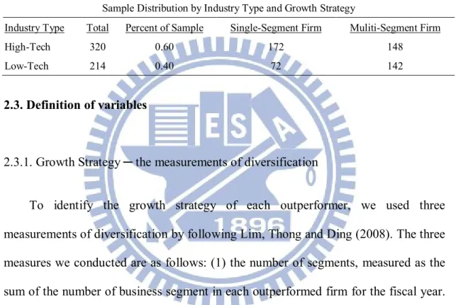
Table 3 presents the sample distribution by the industry type (high- and low-tech industry) and corporate growth strategy. The high- and low- technology industries are categorized by following that of Brown, Fazzari, and Peterson (2009). Table 3 shows that most of outperformed firms, either single- or multi-segment firms, can be found in the high-tech industry. In High-Tech industry, there are more focused firms than
12
diversified firms; on the other hand, there are more diversified firms in Low-Tech industry instead.
Table 3 Sample Distribution by Industry Type and Growth Strategy
This table summarizes the sample distribution by industry type and growth strategy. The final sample consists of 534 outperformers during the period 2002-2004. To identify the organizational form for each outperformer, we partition our overall sample into two subsamples based on whether the outperformers are single-segment firms or multi-segment firms. Data on business segment is from WRDS business-segment files. The high- and low-technology industry types are categorized by following that of Brown, Fazzari, and Peterson (2009).
Sample Distribution by Industry Type and Growth Strategy Industry Type Total
320 Percent of Sample 0.60 Single-Segment Firm 172 Muliti-Segment Firm 148 High-Tech Low-Tech 214 0.40 72 142 2.3. Definition of variables
2.3.1. Growth Strategy ─ the measurements of diversification
To identify the growth strategy of each outperformer, we used three measurements of diversification by following Lim, Thong and Ding (2008). The three measures we conducted are as follows: (1) the number of segments, measured as the sum of the number of business segment in each outperformed firm for the fiscal year. Data on the number of business segments, the segment’s revenue, and the segment’s information are obtained from COMPUSTAT database and Wharton Research Data Services (WRDS). Similarly, the greater number signifies a higher level of diversification. In the second measurement, we used (2) the revenue-based Herfindahl index2, which is a continuous measure that takes higher values with higher level of
2
HIi= ∑ ( , ∑ ,)
Where is firm i’s total number of business segments and , is the firm i’s sales attributable to segment j.
13
diversification. This is a standard method in the strategy and economics literature on diversification (Villalonga, 2004). We calculate as the sum of the squares of each segment’s revenue as a proportion of outperformed firms’ total revenue, after which the inverse of its value was used to easily judge its degree of diversification (i.e., the index equals one for single-segment firm and is smaller than one for multi-segments firms). We compute the sum of squares of each segment’s sales to total sales of the company and then use the inverse of its value in order to easily judge its degree of diversification. That is, the index equals one for single-segment firm and is larger than one for multi-segments firms. Hence, the bigger of the number indicates the higher level of diversification. The third measurement involves the number of segments engaged in a company. We collected (3) dummy for multi-segment firms, which equals zero if there is only one segment and equals one if there are more than two segments (Ruland and Zhou 2005). As defined by SFAS 14, a segment is “a component of an enterprise engaged in providing a product or service or a group of related products and services primarily to unaffiliated customers (i.e., customers outside the enterprise) for a profit.’’
2.3.2. Tobin’s Q
When accessing the firm performance, previous studies have used accounting numbers or stock market return. As Lang and Stulz (1994) point out, this “ex post” methods suffer from two problems, namely, the choice of benchmark for comparisons, which might cause different resluts and the use of adjustment of stock returns for risk. If the risk is not adjusted, a number of firms would perform better, simply because they can bear greater risk. Such phenomenon might distort the evaluation of firm performance. Q, on the other hand, avoids the disadvantages of ex post method
14
because it measures firm performance at a point in time that does not require risk adjustment. Furthermore, Q also contains the capitalized value of the benefits from diversification (Lang & Stulz, 1994).
Similar to Lang and Stulz (1994), Villalonga (2004), and Fernandes and Ferreira (2007), we defined Q as the following equation (2): market value of common equity, plus total assets, minus the book value of common equity, divided by total assets.
Q=
(2)
2.3.3.Other Control Variables
Following Yoon K. Choi (2011), Kim, et al. (1998), Vishal Gaur and Saravanan Kesavan (2007), Pornsit Jiraporn, Young Sang Kim , Ike Mathur (2008), we consider the following control variables, which might be determinants of the value of corporate strategy:
(1) Size: we measured firm size as the logarithm of the total assets.
(2) Liquidity: we measured liquidity as a firm’s cash and equivalents (e.g., cash and marketable securities) in a specific year divided by the book value of total assets in that same year.
(3) Sales Growth: Sales Growth Rate =
(4) Capex ratio: Capex ratio measured as the ratio of capital expenditures to total
sales.
(5) ROA: we define firm profitability using the accounting-based measure, return on assets (ROA).
(6) Leverage: debt ratio measured as the ratio of the book value of total debt over total assets for the year preceding the announcement.
15
2.4. Model
The purpose of this study is to ascertain whether corporate diversification puts a premium or a discount on market value. To examine the relation between diversification and Q, we adopted the following cross-sectional regressions:
Q=f (Diversification, Size, Liquidity, Sales Growth, Capex, ROA, Leverage)
where Q = Tobin’s Q; Diversification, with three measurements: SEG or the number of segment offered by COMPUSTAT, 1/HI or the inverse of Herfidahl index, and DUMMY, with the variable equals one if the firm operates in multiple segments, and zero otherwise. We also employed a few control variables, as suggested by previous studies (e.g., Yoon K. Choi, 2011; Kim, et al., 1998; Vishal Gaur and Saravanan Kesavan, 2007; Pornsit Jiraporn, Young Sang Kim, and Ike Mathur, 2008).
16
3. Empirical Results
3.1 Descriptive Statistics
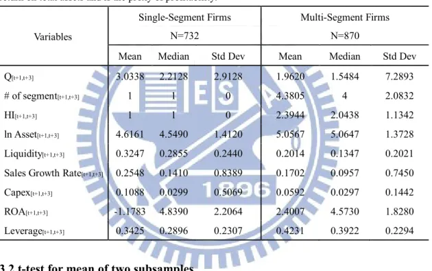
The descriptive statistics are shown in Table 4. Table 4 also presents firm characteristics as well information about outperformers. Of particular interest in our analysis is the relative performance of multi-segment and single-segment firms. The sample consists of 1,602 observations, of which, 732 are from single-segment firms and 870 from multi-segment firms. A quick comparison between the single- and multi-segment samples reveals that single-segment firms tend to be smaller, possess more growth opportunities (i.e., higher sales growth rate), and leverage less. For instance, the average (median) ln assets is 4.6161 (4.5490) for single-segment firms while multi-segment firms have 5.0567 (5.0647). Another example would be the average (median) sales growth rate which is 25.48% (14.10%) for the single-segment firms and 17.02% (9.57%) for the multi-segment firms. Furthermore, the average (median) debt ratio is only 34.25% (28.96%) for the single-segment firms and 42.31% (39.22%) for the multi-segment firms. These observations are comparable to research done by Berger and Ofek (1995), Hadlock, Ryngaert, and Thomas (2001), Chen (2006), and Chen (2008).
17
Table 4 Descriptive Statistics
Descriptive statistics on variables for our sample of firms are from 2002-2004([t+1, t+3]). To identify the growth strategy for each outperformer, we partition our overall sample into two subsamples based on whether the outperformers are single-segment firms (i.e., focused firms) or multi-segment firms (i.e., diversified firms). Q stands for Tobin’s Q and its numerator is computed as book value of total assets and the market value of equity; the denominator is total assets. # of Segment is the number of segment in a company collected from WRDS. HI (herein,”1/HI”) is the Herfindahl Index which is computed based on revenues generated from different segments in a firm. ln assets is the logarithm value of total assets. Liquidity is the ratio that cash and equivalents in a specific year divided by the book value of total assets in that same period. Sales Growth Rate is defined as the annual sales growth rate. Capex is the ratio of capital expenditures to total sales. Leverage is the ratio of debt to total assets. ROA means return on total assets and is the proxy of profitability.
Variables
Single-Segment Firms N=732
Multi-Segment Firms N=870
Mean Median Std Dev Mean Median Std Dev
Q[t+1,t+3] 3.0338 2.2128 2.9128 1.9620 1.5484 7.2893
# of segment[t+1,t+3] 1 1 0 4.3805 4 2.0832
HI[t+1,t+3] 1 1 0 2.3944 2.0438 1.1342
ln Asset[t+1,t+3] 4.6161 4.5490 1.4120 5.0567 5.0647 1.3728 Liquidity[t+1,t+3] 0.3247 0.2855 0.2440 0.2014 0.1347 0.2021 Sales Growth Rate[t+1,t+3] 0.2548 0.1410 0.8389 0.1702 0.0957 0.7450 Capex[t+1,t+3] 0.1088 0.0299 0.5069 0.0592 0.0297 0.1442 ROA[t+1,t+3] -1.1783 4.8390 2.2064 2.4007 4.5730 1.8280 Leverage[t+1,t+3] 0.3425 0.2896 0.2307 0.4231 0.3922 0.2294
3.2 t-test for mean of two subsamples.
Table 5 presents selected features of the sample firms and the t-test for the two
subsamples, focused and diversified. In terms of size, the diversified firms are significantly larger than the focused firms. The liquidity of single-segment firms (32.47%) is significantly higher than that of the diversified firms (20.14%). The sales growth rate and capex ratio are also is significantly higher than that of the diversified firms. The leverage ratio of the diversified firms (42.31%) is significantly higher than that of the single firms (34.25%). The diversified firms have higher profitability that
18
ROA is significantly higher than that of the focused firms. Moreover, the diversified firms have lower Q (1.962) than focused firms (3.0338) at 1% level, implying that diversified firms are likely putting a discount on market value. This result is consistent with Larry H.P. Lang and René M. Stulz (1994), and Kimberly C. Gleason et al. (2011).The t-test used the mean to determine any significantly difference.
Table 5 t-test for mean of two subsamples
Variables for our sample of firms are from 2002-2004([t+1, t+3]). Focused stands for company with only one segment; diversified for more than two segments. Q stands for Tobin’s Q and its numerator is computed as book value of total assets and the market value of equity; the denominator is total assets. # of Segment is the number of segment in a company collected from WRDS. HI (herein,”1/HI”) is the Herfindahl Index which is computed based on revenues generated from different segments in a firm. ln assets is the logarithm value of total assets. Liquidity is the ratio that cash and equivalents in a specific year divided by the book value of total assets in that same period. Sales Growth Rate is defined as the annual sales growth rate. Capex is the ratio of capital expenditures to total sales. Leverage is the ratio of debt to total assets. ROA means return on total assets and is the proxy of profitability.
t-test for mean of two subsamples.
variables Focused Diversified t-statistics
Q[t+1,t+3] 3.0338 1.962 3.74***
HI[t+1,t+3] 1 2.3944 −33.26***
ln Assets[t+1,t+3] 4.6161 5.0567 −6.32***
Liquidity[t+1,t+3] 0.3247 0.2014 11.06***
Sales Growth Rate[t+1,t+3] 0.2548 0.1702 2.14**
Capex[t+1,t+3] 0.1088 0.0592 2.76***
ROA[t+1,t+3] -1.1783 2.4007 −3.93***
Leverage[t+1,t+3] 0.3425 0.4231 −6.98***
N 732 870 -
19
3.3 Correlation Matrix
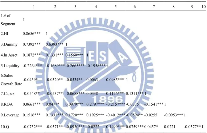
Table 6 presents the Pearson correlations among dependent variable: Q;
independent variables: the proxies of diversification (i.e., number of segment, HI, and Dummy), and other control variables. The correlation between Q and the proxies of diversification (i.e., number of segment, HI, and Dummy) are significantly negative at least at 5% level, which is consistent with Larry H.P. Lang and René M. Stulz (1994) who argued that Q is strongly negatively correlated with the degree of firm diversification. On the other hand, the degree of diversification increases with the number of segments and therefore the correlation is negative for that measure of diversification. The positive correlation between Liquidity or Sales Growth Rate or Capex and Q reveals that cash-rich firms and those with higher growth rates or higher degree of investment level have significantly higher market valuation due to safety concern and future prospect. This result is consistent with that of Fernandes and Ferreira (2007). Furthermore, the correlation between Leverage and Q is significant at 5% level. The correlation coefficients between independent variables and control variables are less than 0.2, and VIFs are all less than 10, proving the absence of any collinear problem.
20
Table 6 Correlation matrix
Variables for our sample of firms are from 2002-2004 Compustat sample of Nasdaq Exchange firms. Q stands for Tobin’s Q and its numerator is computed as book value of total assets and the market value of equity; the denominator is total assets. # of Segment is the number of segment in a company collected from WRDS. HI (herein,”1/HI”) is the Herfindahl Index which is computed based on revenues generated from different segments in a firm. ln assets is the logarithm value of total assets. Liquidity is the ratio that cash and equivalents in a specific year divided by the book value of total assets in that same period. Sales Growth Rate is defined as the annual sales growth rate. Capex is the ratio of capital expenditures to total sales. Leverage is the ratio of debt to total assets. ROA means return on total assets and is the proxy of profitability.
***, **, * statistically significant at the 1%, 5%, and 10% levels, respectively
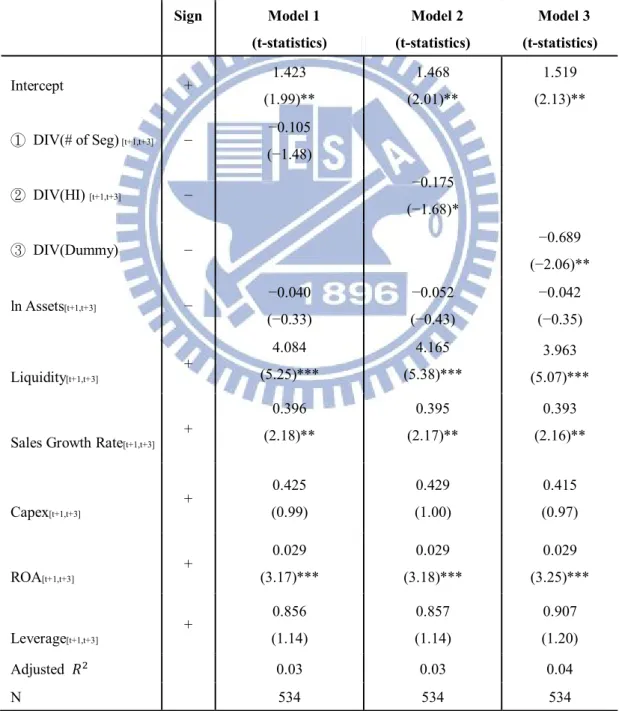
3.4 Cross-sectional Regression Analysis
Table 7 displays the cross-sectional regression results, where the dependent
variable is Q. Model 1, Model 2, and Model 3 seperately presents three different measurements of diversification and their signs. Model 1 uses the number of segments in a company as the proxy of diversification. The coefficient is negative but not statistically significant. Model 2 uses the Herfindahl Index. The coefficient for this
1 2 3 4 5 6 7 8 9 10 1.# of Segment 1 2.HI 0.8656*** 1 3.Dummy 0.7392*** 0.6393*** 1 4.ln Asset 0.1872*** 0.1331*** 0.1560*** 1 5.Liquidity -0.2264*** -0.1689*** -0.2665*** -0.1958*** 1 6.Sales Growth Rate -0.0439* -0.0520** -0.0534** 0.0063 0.0985*** 1 7.Capex -0.0548** -0.0537** -0.0688*** 0.0338 0.1126*** 0.1311*** 1 8.ROA 0.0661*** 0.0477* 0.0979*** 0.2797*** -0.2157*** -0.0375 -0.1541*** 1 9.Leverage 0.1516*** 0.1331*** 0.1720*** 0.1925*** -0.4012*** -0.0594** -0.0255 -0.0953*** 1 10.Q -0.0752*** -0.0571** -0.0930*** -0.0222 0.1499*** 0.0759*** 0.0457* 0.0221 -0.0577** 1
21
variable is negative and significant at the 10% level, implying that average Q increases as the degree of diversification increases. Model 3 includes the dummy variable. The dummy variable is equal to 1 if the firm has more than one segment, and is 0 otherwise. The coefficient for this dummy variable is negative and significant at the 5% level. This evidence is in support of the information asymmetry hypothesis and the agency cost hypothesis.
In summary, the empirical results show negative asscociation between Q and diversificaiton. As a result, all three different measurements of diversification are in support of the diversification discount. Similarly, our evidence is supportive of the view that diversification is not a successful path to higher performance. This result is consistent with Lang and Stulz (1994).
22
Table 7 Cross-sectional Regressions of Q and three measurements of diversification and controls
Variables for our sample of firms are from 2002-2004([t+1, t+3]) Compustat sample of Nasdaq Exchange firms. Q stands for Tobin’s Q and its numerator is computed as book value of total assets and the market value of equity; the denominator is total assets. # of Segment is the number of segment in a company collected from WRDS. HI (herein,”1/HI”) is the Herfindahl Index which is computed based on revenues generated from different segments in a firm. ln assets is the logarithm value of total assets. Liquidity is the ratio that cash and equivalents in a specific year divided by the book value of total assets in that same period. Sales Growth Rate is defined as the annual sales growth rate. Capex is the ratio of capital expenditures to total sales. Leverage is the ratio of debt to total assets. ROA means return on total assets and is the proxy of profitability. The t-statistics are parentheses.
Sign Model 1 (t-statistics) Model 2 (t-statistics) Model 3 (t-statistics) Intercept + 1.423 (1.99)** 1.468 (2.01)** 1.519 (2.13)** ① DIV(# of Seg) [t+1,t+3] − −0.105 (−1.48) ② DIV(HI) [t+1,t+3] − −0.175 (−1.68)* ③ DIV(Dummy) − −0.689 (−2.06)** ln Assets[t+1,t+3] − −0.040 (−0.33) −0.052 (−0.43) −0.042 (−0.35) Liquidity[t+1,t+3] + 4.084 (5.25)*** 4.165 (5.38)*** 3.963 (5.07)***
Sales Growth Rate[t+1,t+3] + 0.396 (2.18)** 0.395 (2.17)** 0.393 (2.16)** Capex[t+1,t+3] + 0.425 (0.99) 0.429 (1.00) 0.415 (0.97) ROA[t+1,t+3] + 0.029 (3.17)*** 0.029 (3.18)*** 0.029 (3.25)*** Leverage[t+1,t+3] + 0.856 (1.14) 0.857 (1.14) 0.907 (1.20) Adjusted 0.03 0.03 0.04 N 534 534 534
23
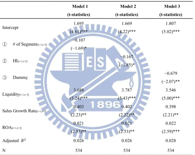
3.5 Regression s of Q and three measurements of diversification and controls. Table 8 demonstrates the effect diversification on Q and other significant control
variables. To examine the relation between diversification and Q, we revised the multivariate regression model as follows:
= ( , , , )
Table 8 displays the multivariate regression results. Model 1, Model 2, and
Model 3 seperately presents three different measurements of diversification and their signs. Model 1 uses the number of segments in a company as the proxy of diversification. The coefficient is negative and statistically significant at 10% level. Model 2 uses the Herfindahl Index. The coefficient for this variable is negative and significant at the 10% level, implying that average Q increases as the degree of diversification increases. Model 3 includes the dummy variable. The dummy variable is equal to 1 if the firm has more than one segment, and is 0 otherwise. The coefficient for this dummy variable is negative and significant at the 5% level. Both results reveal that the degree of diversification increases as the market valuation decreases.
24
Table 8 Regression s of Q and three measurements of diversification and controls
Variables for our sample of firms are from 2002-2004([t+1,t+3]) Compustat sample of Nasdaq Exchange firms.Q stands for Tobin’s Q and its numerator is computed as book value of total assets and the market value of equity; the denominator is total assets. # of Segment is the number of segment in a company collected from WRDS. HI (herein,”1/HI”) is the Herfindahl Index which is computed based on revenues generated from different segments in a firm. Liquidity is the ratio that cash and equivalents in a specific year divided by the book value of total assets in that same period. Sales Growth Rate is defined as the annual sales growth rate. ROA means return on total assets and is the proxy of profitability. The t-statistics are parentheses.
***,**,* statistically significant at the 1%, 5%, and 10% levels, respectively.
3.6 Literature Review ─ Adjusted
Table 9 provides more literature to show low coefficients of determination ( ). The coefficient of determination is used in the context of statistical models whose main purpose is the prediction of future outcomes on the basis of other related information. It is the proportion of variability in a data set that is accounted for by the statistical model. As we can see, the literature related to Q and diversification has
Model 1 (t-statistics) Model 2 (t-statistics) Model 3 (t-statistics) Intercept 1.695 (4.61)*** 1.669 (4.22)*** 1.807 (5.02)*** ① # of Segment[t+1,t+3] −0.107 (−1.69)* ② HI[t+1,t+3] −0.167 (−1.85)* ③ Dummy −0.679 (−2.07)** Liquidity[t+1,t+3] 3.688 (5.24)*** 3.787 (5.43)*** 3.546 (5.00)*** Sales Growth Rate[t+1,t+3]
0.403 (2.23)** 0.402 (2.22)** 0.398 (2.21)** ROA[t+1,t+3] 0.021 (2.53)** 0.021 (2.53)** 0.022 (2.59)*** Adjusted 0.026 0.026 0.028 N 534 534 534
25
much low . Although we have low adjusted in our models, the results seem to be reasonable.
Table 9 Adjusted
Adjusted Literature Review Journal
0.001 0.016 0.024 Philip G. Berger, Eli Ofek (1995) Journal of Financial Economics 37,39-65 0.01 0.03 0.05
Shawn Thomas(2002) Journal of Financial Economics 64, 373–396
0.011 0.015 0.017
Pornsit Jiraporn, Young Sang Kim, Ike Mathur (2008)
International Review of Financial Analysis 17, 1087-1190
3.7 Q and change in the degree of diversification following the black event
We showed that Q falls as diversification increases. The approach we followed so far relates Q cross-sectionally to the degree of diversification. This raises the question of whether firms that diversify are low Q firms or whether they are high Q firms that become low Q firms through diversification. In other words, do poorly performing firms diversify and find out that doing so does not make them high performers or is it that high performers diversify and become poor performers?
We provide evidence from the firms that change the number of segments they report in our sample period to 2. We call these firms diversifying firms under the assumption that the reporting of segment numbers is unbiased. With this assumption, firms that increase the number of segments reported are firms that either has acquired a new, important line of business or firms that have expanded an existing line of business to the point where it is large enough to justify reporting.
Table 10 shows the t-test for mean of Q. Firms that choose to diversify have
26
for the mean. Firms that increase their number of segments have significantly lower Q's than firms that keep their number of segment constant. Diversifying firms have lower Qs. One possible explanation for this tendency of diversifying firms to have lower Q's is that the firms that diversify have lower Q's because the market anticipates poorer performance to result from the diversification attempt.
Table 10 t-test for mean of Q
Variables for our sample of firms are from 2001-2002([t, t+1]).Data on firms that add segments (diversifying firms, i.e., ∆seg > 0) and firms that reduce their number of reported segments (focusing firms, i.e., ∆seg < 0). Data on firms that change their segment (i.e., ∆seg ≠ 0) and firms that do not change their segment (i.e., ∆seg = 0). The t-statistics are parentheses.
Tobin's Q N t-statistics (Pr>|t|) ∆seg[t,t+1] = 0 1.87 344 1.26(0.20) ∆seg[t,t+1] ≠ 0 1.64 180 - ∆seg[t,t+1] > 0 1.35 86 -1.38(0.16) ∆seg[t,t+1] < 0 1.9 94 - ∆seg[t,t+1] = 0 1.87 344 -0.17(0.86) ∆seg[t,t+1] < 0 1.9 94 - ∆seg[t,t+1] = 0 1.87 344 3.26(0.0012)*** ∆seg[t,t+1] > 0 1.35 86 -
***,**,* statistically significant at the 1%, 5%, and 10% levels, respectively.
4. Conclusion
To understand that growth strategy is considered to be of crucial importance to the long-term performance of a firm. This paper examines the differences in market value between focus and diversification strategy. As a result, we find that the outperformance made by focused firms experience greater long-run stock performance (BHARs) than diversified firms, but not significant.
27
Also, the highly diversified firms have significantly lower Q than focused firms. This evidence shows strongly that highly diversified firms are consistently valued less than focused firms. The cross-sectional regression analyses also document a significantly negative relation between the degree of corporate diversification and Tobin’s Q, even after controlling for other determinants. Therefore, we conclude that there is a negative relationship between the degree of diversification and Q in our dataset, which is consistent with information asymmetry hypothesis.
We also provide evidence from the firms that change the number of segments they report in our sample period to 2. Firms that increase their number of segments have significantly lower Q's than firms that keep their number of segment constant. Diversifying firms have lower Qs, and it is consistent with our previous results. One possible explanation for this tendency of diversifying firms to have lower Q's is that the firms that diversify have lower Q's because the market anticipates poorer performance to result from the diversification attempt.
Our evidence is supportive of the view that diversification is not a successful path to higher market values, but it is less definitive on the question if the extent to which diversification hurts market values.
Our results also suggest that a more detailed analysis of the benefits and costs of diversification that tests explicit models of these benefits and costs would be used since our evidence is not consistent with the view that some firms do gain from diversification.
28
References
Aggarwal, R. K., & Samwick, A. (2003). Why do managers diversify their firms? Agency reconsidered. The Journal of Finance , 58 (1), pp. 71-118.
Ansoff, H.I. (1957). Strategies for diversification. Harvard Business Review.
Barber, B. M., and J. D. Lyon. (1997). Detecting long-run abnormal stock returns: The empirical power and specification on test statistics. Journal of Financial
Economics ,41, 359-399.
Berger, P. G., & Ofek, E. (1995). Diversification's effect on firm value. Journal of
Financial Economics , 37, pp. 39-65.
Berger, P. G., and E. Ofek. (1996). Bustup Takeovers of Value-Destroying Diversified Firms. Journal of Finance, 51, 1175-1200.
Bhagat, S.; A. Shleifer; and R. W. Vishny. (1990). Hostile Takeovers in the 1980s: The Return to Corporate Specialization. Brookings Papers on Economic Activity , 1-72. Brown, J., S. Fazzari, and B. Peterson. (2009). Financing Innovation and Growth: Cash
Flow, External Equity, and the 1990s R&D Boom. The Journal of Finance 64, 151–
185.
Comment, R., and G. A. Jarrell. (1995). Corporate focus and stock returns. Journal of
Financial Economics 37, 67–87.
Denis, D. J., Denis, D. K., and A. Sarin. (1997). Agency Problems, Equity Ownership, and Corporate Diversification. Journal of Finance 52, 135-160.
Fama, E. F., & French, K. R. (1992). The cross-section of expected stock returns. The
Journal of Finance , 47 (2), pp. 427-465.
Fama, E. (1998). Market efficiency, long-term returns, and behavioral finance. Journal
29
Fernandes, N., & Ferreira, M. A. (2007). The evolution of earnings management and firmvaluation: A cross-country analysis. working paper, ISCTE Business School . George M. Frankfurtera, Elton G. Mcgoun (2001). Anomalies in Finance: What Are
They and What are They Good For? International Review of Financial Analysis, 10,
p. 22.
Hadlock, C. J., M. Ryngaert, and S. Thomas. (2001). Corporate Structure and Equity Offerings: Are There Benefits to Diversification? Journal of Business 74, 613-635. Hyland, D. C, and J. D. Diltz. (2002). Why Firms Diversify: An Empirical
Examination. Financial Management, 31, 51-81.
Jiraporn, P., Kim, Y. S., & Mathur, I. (2008). Does corporate diversification exacerbate or mitigate earnings management?: An empirical analysis. International Review
of Financial Analysis , 17, pp. 1087–1109.
John C. Bogle. (2008). Black Monday and Black Swans. Financial Analysts Journal
Volume 64, Number 2.
John, K., and E. Ofek. (1995). Asset sales and increase in focus. Journal of Financial
Economics 37, 105–126.
Jonathan E. Clarke, C. Edward Fee, and Shawn Thomas. (2004). Corporate diversification and asymmetric information: evidence from stock market trading characteristics. Journal of Corporate Finance, Volume 10, Issue 1, January 2004,
Pages 105–129
Kim C., Mauer DC, & Sherman AE. (1998). The determinants of corporate liquidity: theory and evidence. Journal of Financial and Quantitative Analysis 33, pp. 335– 359.
30
Kimberly C. Gleason, Inho Kim, Yong H. Kim, and Young Sang Kim. (2011). Corporate Governance and Diversification. Asia-Pacific Journal of Financial
Studies 41, 1–31.
Lang, L. H., & Stulz, R. M. (1994). Tobin's q, corporate diversification and firm performance. Journal of Political Economy , 102, pp. 1248-1280.
Leslie E. Palich, Laura B. Cardinal, and C. Chet Miller (2000). Curvilinearity in the diversification-performance linkage: An examination of over three decades of research. Strategic Management Journal. Strat. Mgmt. J., 21: 155–174.
Lim, C. Y., Thong, T. Y., & Ding, D. K. (2008). Firm diversification and earnings management: evidence from seasoned equity offerings. Review of Quantitative
Finance and Accounting , 30, pp. 69-92.
Loughran, T., & Ritter, J. R. (1995). The new issues puzzle. The Journal of Finance ,
50 (1), pp. 23-51.
Loughrana, T.,and Jay R. Ritter. (2000). Uniformly least powerful tests of market efficiency. Journal of Financial Economics Volume 55, Issue 3, March 2000, Pages
361–389.
Madiha Latif, Shanza Arshad, Mariam Fatima, & Samia Farooq (2011). Market Efficiency, Market Anomalies, Causes, Evidences, and Some Behavioral Aspects of Market Anomalies. Research Journal of Finance and Accounting, vol 2.
Michell, M., and E. Stafford. ( 2000). Managerial Decisions and Long‐Term Stock Price Performance. Journal of Business 73, 287-329.
Morck, R., & Yeung, B. (1998). Why investors sometimes value size and diversification: The Internalization theory of synergy. Working paper .
Moses, O. D. (1987). Income smoothing and incentives: Empirical test using accounting changes. The Accounting Review , 62, pp. 259-377.
31
Paul Zarowin. (1990). Size, Seasonality, and Stock Market Overreaction. The Journal
of Financial and Quantitative Analysis, Vol. 25, No. 1 (Mar., 1990), pp.113-125
Pornsit Jiraporn , Young Sang Kim , Ike Mathur. (2008). Does corporate diversification exacerbate or mitigate earnings management?: An empirical analysis. International
Review of Financial Analysis 17, pp. 1087–1109
Ramanujam, V., & Varadarajan, P. (1989). Research on corporate diversification: A synthesis. Strategic Management Journal , 10, pp. 523-551.
Rajan, R., H. Servaes, and L. Zingales. (2000). The cost of diversity: The diversification discount and inefficient investment. Journal of Finance 55, 35-80. Ruland, W., and Ping Zhou. (2005). Debt, diversification, and valuation. Review of
Quantitative Finance and Accounting 25, 277-291.
Sanjai Bhagat , & Brian Bolton. (2008). Corporate governance and firm performance.
Journal of Corporate Finance 14 (2008) 257–273
Servaes, H. (1996). The Value of Diversification During the Conglomerate Merger Wave. Journal of Finance, 51, 1201-1226.
Shawn Thomas. (2002). Firm diversification and asymmetric information: evidence from analysts’ forecasts and earnings announcements. Journal of Financial
Economics 64, 373–396.
Sheng-Syan Chen. (2006). The economic impact of corporate capital expenditures: Focused firms versus diversified firms. The Journal of Financial and Quantitative
Analysis, Vol. 41, No. 2 (Jun., 2006), pp.341-355
Sheng-Syan Chen. (2008). Organizational form and the economic impact of corporate new product strategies. Journal of Business Finance and Accounting 35, 71-110. Shin, H. H., and R. M. Stulz. (1998). Are internal capital markets efficient? Quarterly
32
Teoh, S. H., Welch, I., & Wong, T. J. (1998). Earnings management and the long-run market performance of initial public offerings. The Journal of Finance1 , 53 (6),
pp.1935-1974.
Villalonga, B. (2004). Diversification Discount or Premium? New Evidence from the Business Information Tracking Series. The Journal of Finance , 59, pp. 479-506. Vishal Gaur, Saravanan Kesavan. (2007). The Effects of Firm Size and Sales Growth
Rate on Inventory Turnover Performance in the U.S. Retail Sector.
Wemerdelt, B., and C. A. Montgomery. (1998). Tobin’s q and the importance of focus in firm performance. American Economic Review 78, 246-250.
Yoon K. Choi. (2011). Corporate Governance, Diversification, and Firm Value: Evidence from “Spin-Ins”. 24th Australasian Finance and Banking Conference 2011
33
Appendix
Table 11 Cross-sectional Regressions of Q and teck dummy and controls
Variables for our sample of firms are from 2002-2004([t+1,t+3]) Compustat sample of Nasdaq Exchange firms.Focused stands for company with only one segment; diversified for more than two segments. Q stands for Tobin’s Q and its numerator is computed as book value of total assets and the market value of equity; the denominator is total assets. ln assets is the logarithm value of total assets. Liquidity is the ratio that cash and equivalents in a specific year divided by the book value of total assets in that same period. Sales Growth Rate is defined as the annual sales growth rate. Capex is the ratio of capital expenditures to total sales. Leverage is the ratio of debt to total assets. ROA means return on total assets and is the proxy of profitability. teck dummy for high-teck firms , which equals one if firm’ SIC code is categorized in high-tech industries 283, 357, 366, 367, 382, 384, and 737 with coverage in Compustat, otherwise equals to zero.( Brown, Fazzari, and Peterson, 2009).
Sign Model (t-statiatics) Intercept + 1.3384 *(1.76) ln Assets[t+1,t+3] − −0.0730 (−0.60) Liquidity[t+1,t+3] + 4.3829***(5.35) Growth of Sales[t+1,t+3] + 0.4000**(2.20) Capex[t+1,t+3] + 0.4358(1.02) ROA[t+1,t+3] + 0.0286(3.16) Leverage[t+1,t+3] + 0.7580(0.99) teck dummy − −0.1598(−0.42) N 534 Adjusted 0.0287
***,**,* statistically significant at the 1%, 5%, and 10% levels, respectively.
Table 11 displays the cross-sectional regression results, where the dependent variable is Q. Model includes the teck dummy variable. The teck dummy variable is equal to 1 if the firm’ SIC code is categorized in high-tech industries 283, 357, 366, 367, 382, 384, and 737 with coverage in Compustat, and is 0 otherwise.( Brown, Fazzari, and Peterson, 2009). The coefficient for this dummy variable is negative but not significant. And the adjusted is still much low, which means that high- or low-teck firms are not the key factor for the performance.