Quantitative theory of transport in vortex matter of type-II superconductors
in the presence of random pinning
B. Rosenstein and V. Zhuravlev
National Center for Theoretical Sciences and Electrophysics Department, National Chiao Tung University, Hsinchu 30050, Taiwan, Republic of China
共Received 27 January 2007; revised manuscript received 24 April 2007; published 17 July 2007兲
We quantitatively describe the competition between interactions, thermal fluctuations, and random quenched disorder using the dynamical Martin-Siggia-Rose approach 关Phys. Rev. A 8, 423 共1973兲兴 to the Ginzburg-Landau model of the vortex matter. The approach first used by Dorsey et al.关Phys. Rev. B 45, 523 共1992兲兴 to describe the linear response far from Hc1is generalized to include both pinning and finite voltage. It allows one
to calculate the non-Ohmic I-V curve, thereby extending the theory beyond the linear response. The static flux line lattice in type-II superconductors undergoes a transition into three disordered phases: the vortex liquid共not pinned兲, the homogeneous vortex glass 共pinned, if one disregards an exponentially small creep at finite tem-peratures兲, and the crystalline Bragg glass 共pinned兲 due to both thermal fluctuations and disorder. The location of the glass transition line in the homogeneous phase is determined and compared to experiments. The line is clearly different from both the melting line and the second peak line describing the translational and rotational symmetry breaking at high and low temperatures, respectively. Time correlation and response functions of the order parameter as functions of the time difference are calculated in both the liquid and the amorphous homogeneous phases. They determine the relaxation properties of the vortex matter due to the combined effect of pinning and thermal fluctuation. We calculate the critical current as a function of magnetic field and temperature in the homogeneous phase. The surface in the J-B-T space defined by this function separates between a dissipative moving vortex matter regime and vortex glass. A quantitative theory of the peak effect, qualitatively different from the conventional one due to Pippard关C. Tang, X. Ling, S. Bhattacharya, and P. M. Chaikin, Europhys. Lett. 35, 597共1996兲; A. B. Pippard, Philos. Mag. 19, 217 共1969兲; A. I. Larkin and Yu. N. Ovchinnikov, J. Low Temp. Phys. 34, 409共1978兲兴, is proposed.
DOI:10.1103/PhysRevB.76.014507 PACS number共s兲: 74.40.⫹k, 74.25.Ha, 74.25.Dw
I. INTRODUCTION
In type-II superconductors for which the penetration depth exceeds the correlation length, the magnetic field penetrates the sample in the form of Abrikosov vortices which strongly interact, thereby creating an elastic “vortex matter.” Impurities always present in a sample lead to inho-mogeneities both on the microscopic scale共described by the electron’s mean free path兲 and the mesoscopic scale 共pin-ning兲, which greatly affect the thermodynamic and, espe-cially, dynamic properties of the vortex matter. When disor-der is strong enough, it pins the vortex matter, resulting in dissipationless persistent current, thereby recovering an original defining property of superconductor. In addition, thermal fluctuations also significantly influence the vortex matter, either directly by melting the vortex lattice into a vortex liquid or by changing the efficiency of the disorder 共thermal depinning兲. They are especially important in high Tc
superconductors. As a result of a delicate interplay between disorder, interactions, and thermal fluctuations, even the static H-T phase diagram of high Tcsuperconductors is very
complex and is still far from being reliably determined. Once electric current J is injected into a sample, one is faced with the problem of describing the dynamical phase diagram, which should be drawn in the three dimensional space T-H-J. This makes the analysis essentially more com-plicated, especially if one intends to study it beyond linear response. Generally, there are two phases: the pinned phase, in which the vortices are pinned and thus the resistivity
van-ishes 共perfect superconductivity exists兲, and the unpinned phase, in which vortices can move due to Lorentz force and thus a finite resistivity appears. The transition surface is de-termined by the critical current as function of magnetic field H and temperature T. When the critical current vanishes, the intersection of the surface with the H-T plane gives the “static” irreversibility line.
Theoretically, the problem of the vortex matter subject to both thermal fluctuations and disorder has a long history. Two major simplifications are generally made. In the major-ity of the works, the vortex matter is considered as an array of elastic lines.2 This 共London兲 approximation is generally
valid far from the higher critical field Hc2, when the vortex
density is low. An alternative simplification to the vortex matter is valid far enough from the lower critical field Hc1.
At high vortex densities, magnetic fields of many vortices overlap and the resulting magnetic inductance is nearly ho-mogeneous. It is usually supplemented by the so-called low-est Landau level 共LLL兲 approximation.3,4 The original idea
of the vortex glass5 and the continuous glass transition
ex-hibiting the glass scaling of conductivity in statics appeared early in the framework of the frustrated XY model.6 The
model was studied by the renormalization group and the variational methods, and has been extensively simulated numerically.7,8 In analogy to the theory of spin glasses, in
this model the replica symmetry is broken when crossing the glass transition line. The frustrated XY model ran into several problems. For finite penetration depth, it has no transition9
and, moreover, there was a difficulty in explaining sharp
Bragg peaks observed in the experiments at low magnetic fields. To address the last problem, another simplified model had been proven to be more convenient: the elastic medium approach to a collection of interacting linelike objects sub-ject to both the pinning potential and the thermal bath. The resulting theory was treated using the Gaussian approximation10,11 and renormalization group.6The original
problem of the very fast destruction of the vortex lattice by disorder was solved with the vortex matter being in the rep-lica symmetry broken phase for dimensionality 2⬍D⬍4, and it was termed “Bragg glass.” In D = 2, there exists dis-crete replica symmetry broken transition. It is possible to address the problem of dynamics in the presence of thermal fluctuation using an approach in which one directly simulates the interacting line-like objects subject to both the pinning potential and the thermal bath Langevin force.12
A vast majority of theoretical works deal with the linear response and cannot address the flux dynamics at finite cur-rents. The I-V curves of the flux flow are very nonlinear. However, one should be very cautious in interpreting the experimental results since they generally do not distinguish between the bulk and the edge effects. In several experiments in which the bulk was isolated共either by Corbino geometry13
or by varying the width of the sample14兲, one finds that the
bulk I-V has a structure simpler than the commonly accepted nonlinear form. It is important to achieve a theoretical un-derstanding of both the bulk and edge contributions in the region of the magnetic phase diagram in which these experi-ments on NbSe2were performed. Very often the flux
dynam-ics is investigated in the London limit with widely separated vortices, so that one can model them as an array of line-like thin objects interacting pairwise. The motion in the presence of disorder looks like a rather chaotic advance in channels, with sudden hops between pinning centers and occasional avalanches. This picture cannot be directly applied in situa-tions when magnetic field of vortices overlap, creating a ho-mogeneous magnetic field. Still, the core regions might ex-hibit this type of behavior. Moreover, the connection between the qualitative description of the motion and the resulting I-V curves is not clear at present.
In this paper, we investigate the 共bulk兲 dynamics of the vortex matter beyond linear response using the disordered Ginzburg-Landau model. In statics, the replica method of handling disorder in the framework of LLL Ginzburg-Landau 共GL兲 model was utilized in both three dimensions and two dimensions15,16 to obtain the irreversibility line
along with other properties of the disordered vortex matter. The irreversibility lines of YBCO and a two-dimensional 共2D兲 organic superconductor were found to be in good agree-ment with experiagree-ment.16 Tesanovic and Herbut used super-symmetry共for columnar defects in layered materials兲.17
Dy-namics in the presence of thermal fluctuations and disorder is phenomenologically described using the time dependent Ginzburg-Landau 共TDGL兲 model, in which the coefficients have random components.2,18Such an attempt was made by
Dorsey et al.1 in the homogeneous 共liquid兲 phase using a
dynamic Martin-Siggia-Rose 共MSR兲 formalism.19,20 They
obtained the irreversibility line and formulated the linear re-sponse theory of the vortex matter.
The main purpose of this paper is to study the dynamics of three-dimensional vortex matter beyond linear response
using the dynamical approach1 within the TDGL model at
finite electric field. In strongly type-II superconductors共for which the Ginzburg-Landau ratio=/is large兲, magnetic and electric fields inside the superconductor are homoge-neous over a wide range of parameters. As mentioned above, high homogeneity of magnetic field in the mixed state origi-nates from superposition of many共B˜/Hc1Ⰷ1兲 vortices. The
same argument is valid for an electric field which arises due to vortex motion. Indeed, the electric field is related by Lor-entz transformation to the homogeneous magnetic field ap-pearing in the frame moving with vortices. Linear response, namely, conductivity in the limit of zero current, is typically obtained using the Kubo formula.1,21–23A theory with a finite
electric field allows one to obtain the I-V curve beyond the linear response. Finite electric fields without disorder have been considered within the framework of TDGL in Refs.4,
21, and24.
Complex motion of vortex matter featuring mesoscopic avalanches, channels, and islands of pinned flux described above, which might exist, are not probed directly in our method of averaging over the white noise disorder. Analyti-cally, one preforms the disorder average of conductivity and magnetization, and does not directly see the picture above. To get a glimpse into the dynamics, time dependent tion functions are calculated. We study the dynamic correla-tion funccorrela-tion C共r,, r
⬘
,⬘
兲 and the response functions R共r,, r⬘
,⬘
兲 共averaged over disorder and thermal fluctua-tions兲 of the order parameter within an appropriately gen-eralized Gaussian approximation in both the flux flow and the pinned phases. We consider the stationary case only,1namely, when the correlation function depends on the time difference and is therefore characterized by the spectrum C. The critical surface Tg共H,J兲 in the three-dimensional space
T-H-J, separating the pinned and unpinned phases, is ob-tained as a surface at which C→⬁ for →0. Above this surface, the real space correlator decays exponentially, while below it is a constant at large time scales. The constant is proportional to the Edwards-Anderson order parameter char-acterizing transition to a glassy state.25Approaching
critical-ity in the parameter space T→Tg
, various quantities diverge powerwise in共T−Tg兲, with critical exponents calculated in mean field. The static glass transition line, namely, the line at zero electric field, coincides with the one obtained using the replica method.16A relation between the dynamical and
rep-lica methods, which is important for understanding the na-ture of any glass transition, is discussed.
We show that the leading contribution to conductivity near the glass line comes from the first Landau level rather than from the LLL. The conductivity diverges on the static glass line. This has important physical consequences. It is well known that within LLL both magnetization and conduc-tivity are proportional to the superfluid density兩兩2.
Magne-tization is generally proportional to the superfluid density in the first order in 1 /2共see Ref.26兲, while for arbitrary LLL
configuration, the electric current can be written as J⬀共zˆ ⫻ⵜ兲兩兩2. This relation does not hold for higher Landau
lev-els共LLs兲. Experimentally, however, while magnetization is continuous across the line, the conductivity diverges. This is known to happen in a wide range of materials and
param-eters. Compare, for example, a recent experiment27on
mag-netization in BSCCO and an earlier transport measurement in the same material and the same range of parameters.28The fact that near the glass line contribution from higher LL 共HLL兲 takes over removes this difficulty of the LLL theory. The exponentially small vortex creep is not included共it cor-responds to instanton contribution in the formulation adopted兲, and therefore, is not general in this respect.
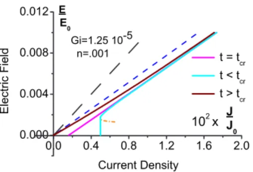
The main result of the present paper is the calculation of the I-V curves in a wide range of parameters. The I-V looks often as a shifted straight line, rather different from the smooth power-like behavior seen in many experiments. However, as mentioned above, it is consistent with recent measurements in which the edge contribution was mini-mized.13,14,29In addition, we provide an alternative theory of
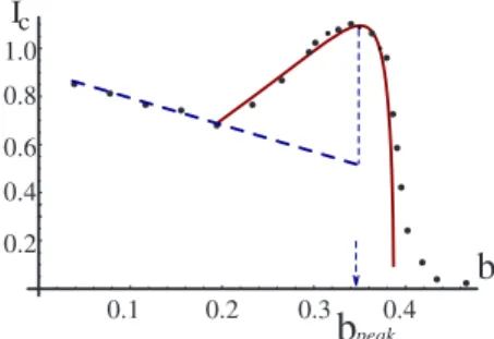
the peak effect in the critical current. A sharp increase of the critical current is not considered as gradual, due to softening of the vortex lattice before melting, but rather an abrupt jump into the homogeneous vortex glass state, in which we obtain large current diminishing fast while approaching the glass line.
The paper is organized as follows. The disordered TDGL model at a constant electric field is defined in Sec. II. The Martin-Siggia-Rose formalism is applied to it using the basis of Landau levels in electric field. In Sec. III, we briefly de-scribe a variant of the Gaussian approximation functional integral method30,31 and apply it to the MSR action for the
LLL sector. We find the dynamical glass transition surface and calculate various critical exponents. The stationary cor-relations in the pinned phase are also found. It is shown in Sec. IV that the main contribution to the current near the glass transition line comes from higher Landau levels, and their leading contribution is calculated. The rest of the paper deals with applications of the obtained general results to ex-periments. The irreversibility line and the I-V curves are con-sidered in Sec. V, while the critical current and the theory of the peak effect are discussed in Sec. VI. A brief discussion of the applicability of the theory and conclusions are the sub-jects of Sec. VII.
II. TIME DEPENDENT GL MODEL IN THE PRESENCE OF BOTH DISORDER AND
THERMAL FLUCTUATIONS A. Basic equations and assumptions
Our starting point is the TDGL equation26in the presence
of thermal fluctuations, which on the mesoscopic scale are represented by a共complex兲 white noise21,24:
ប2␥
4m*D= − ␦
␦*F +, 共1兲
where m* is the effective mass of the Cooper pair. The
co-variant time derivative is D⬅ +ieប*⌽, where ⌽ is the sca-lar electric potential describing the driving force in a purely dissipative dynamics. We assume that the charge of the Coo-per pairs is negative −e*, with positive e*= 2e. The inverse
diffusion constant␥/ 2 controlling the time scale of dynami-cal processes via dissipation is real, although a small
imagi-nary共Hall兲 part is generally present.32 The variance of the
thermal noisedetermines the temperature T = tTc:
具共r,兲*共r
⬘
,⬘
兲典 =␦共−⬘
兲␦共r − r⬘
兲ប 2␥2m*T. 共2兲
The static GL free energy including the⌬Tcdisorder1,2is
F =
冕
d3r冋
ប 2 2m*冏
冉
ⵜ + ie* បcA冊
冏
2 + ប 2 2mc *兩z兩2 −␣Tc共1 − t兲关1 + U共r兲兴兩兩2+ b⬘
2兩兩 4册
. 共3兲The random component of Tc, U共r兲, will be modeled by a
white noise characterized by variance depending on the pin-ning:
U共r兲U共r
⬘
兲 =␦共r − r⬘
兲2znp. 共4兲
The dimensionless pinning strength npis proportional to the
density of pinning centers in units of the coherence volume 2
z, where z=␥awith anisotropy parameter␥a=
冑
m*mc*. We neglect possible random components of other coefficients in TDGL. These might lead to important physical consequences and were considered using replica formalism in statics in Ref. 16. The space covariant derivative D⬅ⵜ+ieបc*A,
de-scribes magnetic field, and the coefficients are related to the coherence length and the magnetic penetration depth via ␣Tc= ប
2
2m*2 and b
⬘
=2ប22e*2
2c2m*2 . The TDGL equations, therefore,
can be written in a form
Lˆ=␣Tc共1 − t兲U− b
⬘
兩兩2+, 共5兲where a共non-Hermitian兲 linear operator is defined by Lˆ⬅ ប 2␥ 4m*D− ប2 2m*D 2− ប 2 2mc* z 2 −␣Tc共1 − t兲. 共6兲
We make several assumptions共identical to those made in Ref.21 and major parts of Ref.4兲 to simplify the problem.
As was discussed in the Introduction, in strongly type-II su-perconductors, =/Ⰷ1; magnetic and electric fields are very homogeneous since fields of vortices overlap. Therefore the Maxwell type equations for electromagnetic field are not considered. The axes are chosen in such a way that the mag-netic and electric fields are oriented along the negative z direction and the negative y direction, respectively. The vor-tices are moving along the positive x direction due to the Lorentz force. The electric and magnetic fields E = −ⵜ⌽ −tA; B =ⵜ⫻A are written in the Landau gauge, with the
vector potential A =共By,0,0兲 and the scalar potential ⌽ = Ey, respectively. Temperatures, currents, and magnetic fields should be close “enough” to the dynamical phase tran-sition line Hc2共T,E兲 in order to apply the GL approach based
on an assumption that the order parameteris small.
B. Martin-Siggia-Rose formalism for TDGL model A Langevin type dynamics can be formulated as a func-tional problem with the dynamical “partition function,”
de-fined by the MSR functional integral19over the order
param-eter and an additional “ghost” field33 . The ghost field
allows exact integration over the white noise. As was no-ticed by Sompolinsky and Zippelius,20 who considered a
similar model in the context of the spin glass theory, this allows one to exactly average over disorder by performing a Gaussian integration over the random field U共x兲 correlated according to Eq.共4兲 without invoking the replica trick:
Z =
冕
D*DD*Dexp兵− AMSR关,兴其. 共7兲Since共a rather nontrivial兲 derivation is closely analogous to the one presented in detail in Ref. 20, with certain aspects further clarified in Ref. 34, we just presented the resulting actionAMSR关,兴. This choice is more convenient for
per-forming Gaussian approximation and does not lead to any mathematical complications.
The functional approach enables us to calculate both the dynamics correlators and response function of the system in close analogy to the calculation of the static correlators in statistical physics. For example, the dynamical correlator and the response function are
C共r,,r
⬘
,⬘
兲 = 具r共兲r⬘ *共 ⬘
兲典 = Z−1冕
D*DD*D r共兲 ⫻r⬘ *共⬘
兲exp兵− A MSR关,兴其, 共8兲 R共r,,r⬘
,⬘
兲 = 具r共兲r⬘ *共 ⬘
兲典 = Z−1冕
D*DD*D r共兲 ⫻r⬘ *共⬘
兲exp兵− A MSR关,兴其. 共9兲From now on,具¯典 will denote both the thermal and disorder averages. The dimensionless “action” contains a quadratic part and two quartic parts共omitting certain counterterms that will be mentioned below in Sec. III B兲,
Afree= 1 T␥2
冕
r, 兵r *共兲Lˆ r共兲 + c.c.其 − ប 2 2Tm*␥4冕
r, r共兲r*共兲 − 4b⬘
l2 z ␥2␣T c冕
r, r共兲r*共兲, 共10兲 Adis= − 2z ␥22np冋
␣共1 − t兲 t册
2冕
r,, 关r *共兲 r共兲 +r共兲r *共兲兴 ⫻关r*共兲r共兲 +r共兲r*共兲兴, 共11兲 Aint= b⬘
T␥2冕
r,r共兲r *共兲关 r *共兲 r共兲 +r共兲r*共兲兴, 共12兲where the operator Lˆ was defined in Eq.共6兲. The second term
in Eq.共10兲 appears due to thermal noise averaging, while the
last one represents a functional Jacobian arising from nor-malization of the ghost field integration.19,34The two quartic
parts describe the disorder and the interactions, respectively.
In the theoretical part of this paper, we will use appropri-ate units of time
⬘
=/GLwith characteristic GL time scaleGL=␥2 and coordinates x
⬘
= x / l, y⬘
= y / l, z⬘
= z /z, wheremagnetic length is l =b−1/2 with b = B / Bc2. It is convenient
to combine the fields in a dimensionless two component col-umn ⌿ =
冉
␣l2z t冊
1/2冉
冊
, in terms of which the action takes the formAfree=
冕
r, ⌿r *共兲D−1⌿ r共兲, Adis= − ng冕
r冋
冕
⌿r *共兲 x⌿r共兲册
2 , Aint= g 2冕
r 关⌿r*共兲↑⌿r共兲兴关⌿r*共兲x⌿r共兲兴. 共13兲Here, we introduced two dimensionless couplings n = np
4
冑
2Gi 共1 − t兲2t , 共14兲
characterizing the relative strength of disorder compared to interactions, and
g = 8bt
冑
2Gi, 共15兲characterizing the interactions compared to thermal fluctua-tions with
冑
2Gi =4␣b2T⬘c2z. The inverse propagator matrix is D−1=
冉
− 2g Lˆ+
Lˆ − 1
冊
, 共16兲where the operator Lˆ of Eq.共6兲 has the form
Lˆ =1 2共+ 4ibvy兲 − b关共x− iy兲 2+ y 2兴 − z2−共1 − t兲, 共17兲 with velocity of fluxons
v =e
*␥El3
4ប 共18兲
given in units of c. We make use of Pauli matricesx,y,z,
and↑,↓=12共1±z兲.
Since the spectrum of the operator Lˆ is discrete共the Lan-dau quantization兲, in a certain range of parameters, one can significantly simplify the problem by considering the “low energy” states only. It is therefore advantageous to reexpress the model in the Landau level basis.
C. Landau level basis in the presence of electric field The moving Landau harmonics are solutions of linearized time dependent GL equation in the presence of electric field.
Mathematically, we define them as the right eigenfunctions of the operator Lˆ, Eq. 共17兲, with eigenvalues LNk,k
z:
Lˆ共e−i
Nk,kz兲=LNk,kz共e−iNk,kz兲, where
Nk,kz= 1
冑
2NN!1/2e −v2/2H N共y − k + iv兲exp关ikzz兴 ⫻exp关ikx兴exp冋
−1 2共y − k + iv兲 2册
, 共19兲and HN共y兲 are Hermit polynomials. The basis functions are
normalized as
冕
r
¯Nk⬘共r兲Mk共r兲 = 共2兲2␦k⬘k␦N,M 共20兲
and␦k⬘k is the 2D␦ function with k =兵k,kz其. Since the
op-erator is not Hermitian, they are different from the left eigen-functions ¯Nk,k
z defined as Lˆ
†共ei¯
Nk,kz兲=LNk,k* z共ei¯Nk,kz兲,
see Ref.24.
The order parameter and the ghost fields are expanded, therefore, via the moving Landau harmonics as
⌿r共兲 =
1 共2兲3/2
兺
N=0
冕
ke−iNk共r兲⌿Nk,. 共21兲
We will use in Sec. III the LLL subspace, although higher levels will be necessary for the calculation of supercurrent and will be considered in Sec. IV. It will be convenient to separate the presumably more important LLL subspace from the rest, the HLL part:
⌿r共兲 = ⌽r共兲 + ⌰r共兲, 共22兲
where⌽k,⬅⌿0k, and ⌰k,⬅兺N=1⌿Nk,. As will become clear in Sec. IV, it will be sufficient for our purposes to consider effects up to first order in⌰r共兲, and now, we
con-centrate on the LLL sector.
In the LLL sector, the quadratic part of the action takes the form Afree=
冕
k, ⌽k,*Dk−1⌽k,, Dk−1=冢
− 2g i⬘
2 + kz 2 + 2ah − i⬘
2 + kz 2+ 2a h − 1冣
, 共23兲where
⬘
=− 4bvk and ah= −共1−t−b−bv2兲/2 is the“dis-tance” on the dynamical phase diagram from the mean field normal-superconductor transition line. The quartic terms are
Adis= − ng 共2兲5/2
冕
关k兴,,␦k1−k2+k3−k4 f0共关k兴兲共⌽k1, * x⌽k2,兲 ⫻共⌽k3, * x⌽k4,兲, 共24兲 Aint= g 2共2兲7/2冕
关k兴,关兴␦1−2+3−4 k1−k2+k3−k4 f 0共关k兴兲共⌽k1,1 * ↑⌽k2,2兲 ⫻共⌽k3,3 * x⌽k4,4兲, 共25兲where关k兴 and 关兴 denote a set of all variables 兵k1, k2, k3, k4其
and 兵1,2,3,4其, respectively, and ␦1−2+3−4
k1−k2+k3−k4 is a
product of Dirac ␦ functions ␦共1−2+3−4兲␦共k1− k2
+ k3− k4兲. The Gaussian damping factor f0共关k兴兲
= exp
关
−共k2−k1兲2+共k 4−k1兲2
2
兴
arises from matrix elements of fourLLL functions.
III. CONSISTENT GAUSSIAN APPROXIMATION FOR THE MSR ACTION
Since the model is highly nontrivial even in the simplest cases, one has to use an approximation scheme. We utilize a method which evolved from the Gaussian variational ap-proach to quantum mechanics, referred to here as Gaussian approximation.31Generally, it captures the basic physical
as-pects, although its precision might not be very high共perhaps similar to a dynamical mean field theory in the band struc-ture calculations兲.
Since we will calculate higher correlators using well known, sometimes inconsistently, Gaussian approximation, we start with a brief description of the general method intro-duced in detail in Ref. 30, utilizing the so-called Gaussian effective action and “truncated” Dyson-Schwinger equations. Naively using the Hartree-Fock procedure 共Wick contrac-tions兲 to calculate correlators leads to several important in-consistencies. For example, approximate correlators of Gold-stone bosons are not massless, contrary to the GoldGold-stone theorem. This is crucial in calculating effects dependent on massless modes like the divergence of conductivity on the glass line. An additional advantage of this approach over the resummation of the diagram technique used in Refs.1and23
共borrowed from the physics of weak localization兲 is that it is systematic and unambiguous, without any reference to the “large number of components” limit.
A. Gaussian effective action and correlators
The exact effective action A共⌿¯ ,G兲 introduced by Corn-wall et al.35 is defined as the functional of two variational
parameters, a “classical”共or shift兲 field ⌿¯
A=具⌿A典 = Z−1
冕
⌿,⌿*⌿Aexp兵− AMSR关⌿,⌿
*兴其 共26兲
and a two-field connected correlator GAB=具共⌿A−⌿¯A兲共⌿B * −⌿¯B *兲典 = Z−1
冕
⌿,⌿*共⌿A−⌿ ¯ A兲共⌿B * −⌿¯B *兲exp兵− A MSR关⌿,⌿*兴其. 共27兲 Here, indices of the field⌿ stand for the full set of variables and parameters: A =兵, k , i其, where i=1,2 is the ⌿ columnindex. Minimization of the effective action yields the “shift” and the “gap” equations
␦A共⌿¯ ,G兲 ␦⌿¯ A = 0, ␦A共⌿¯ ,G兲 ␦GAB = 0, 共28兲 respectively.
In the Gaussian approximation,A共⌿¯ ,G兲 is approximated 共up to an unimportant constant兲 by
A共⌿¯ ,G兲 ⯝ AG共⌿¯ ,G兲 = Afree关⌿¯ 兴 − Tr log G + Tr兵D−1G其
+具Adis典G+具Aint典G, 共29兲
whereAfree关⌿¯ 兴 is the quadratic part of AMSR关⌿¯ 兴 action in
Eq.共10兲 and 具Adis典G, 具Aint典Gare calculated as the Gaussian
averages with the field shifted by⌿¯ :
具O典G=
冕
⌿,⌿* O关⌿,⌿*兴exp关− 共⌿*−⌿¯*兲G−1共⌿ − ⌿¯ 兲兴冕
⌿,⌿* exp关− 共⌿ *−⌿¯*兲G−1共⌿ − ⌿¯ 兲兴 .This allows calculation of correlators of the fields via func-tional differentiation with respect to the shift fields. In the rest of this section, we will solve the gap equations for the MSR action, while correlators共including the four-point func-tions兲 are considered in Sec. IV.
B. Application to the LLL model: The gap equation The Gaussian approximation has been applied to the LLL time dependent Ginzburg-Landau model in the absence of electric field using diagram resummation in Ref.1. Here, we use the Gaussian effective action approach leading to an identical gap equation. Assuming that the gauge 共electric charge兲 U共1兲 symmetry is unbroken, the one-field averages 具典, 具典 and the “charged” two-field cor-relators like 具典 should vanish. The invariant 共“neutral”兲 two-point Green functions include the correlator C共r,,
r
⬘
,⬘
兲⬃具r共兲r⬘ *共⬘
兲典, the response function R共r,, r⬘
,⬘
兲 ⬃具r共兲r⬘*共
⬘
兲典, and the auxiliary field correlatorB共r,, r
⬘
,⬘
兲⬃具r共兲r⬘ *共⬘
兲典 共which will vanish; see be-low兲. In a homogeneous dynamical phase 共physically corre-sponding to a stationary flux flow兲, the correlators depend on the differences−⬘
and r⬘
− r only. Therefore, in the兵, k其 space, one hasGAA⬘=␦⬘␦kk⬘Gk, Gk=
冉
Ck Rk
Rk* Bk
冊
, 共30兲 where ␦⬘⬅␦−⬘ and ␦kk⬘=␦k−k⬘ are the one- andtwo-dimensional Dirac delta functions ␦共−
⬘
兲 and ␦共k − k⬘
兲␦共kz− kz⬘
兲, respectively.Making use of the above relation, the quartic terms in Eq. 共29兲 become 具Adis典g= − ng 共2兲5/2␦␦k
冕
关k兴,关k⬘兴, fR共k⬘
− k兲Tr共xGkxGk⬘兲, 共31兲 具Aint典g= g␦␦k 2共2兲7/2冕
关k兴,关k⬘兴,,fR共k⬘
− k兲关Tr共↑GkxGk⬘兲 + Tr共↑Gk兲Tr共xGk⬘兲兴, 共32兲 where ␦=21兰 and ␦k= 1共2兲2兰r are infinite constants, and
fR共k兲=exp
关
− k22
兴
is a reduced version of the damping factorf0共关k兴兲 due to the momentum conservation. In the disorder
term, we omitted the Wick contractions within the curly brackets in Eq.共24兲, since they are canceled exactly by the
disorder “counterterms” in the MSR action, see Ref.34. Cal-culating the functional derivative ofAg共⌽¯ ,G兲, the gap
equa-tion is written in a well known form GAB −1 = DAB −1 + MAB, MAB= ␦ ␦GAB
共具Adis典gauss+具Aint典gauss兲.
Note that GABis a symmetric function with respect to
trans-position of all its indices. Substituting the matrix MAB as a
function of GABinto the gap equation, we arrive at
Gk−1= D˜k−1− 2ng 共2兲5/2
冕
关k⬘兴 fR共k⬘
− k兲xGk⬘x 共33兲 with D˜k−1= Dk−1+ g 共2兲7/2冕
关k⬘兴, fR共k⬘
− k兲 ⫻关↑Tr共xGk⬘兲 +xTr共↑Gk⬘兲兴. 共34兲Here, one clearly sees the difference between the disorder and the interaction contributions in the Gaussian approxima-tion. The interaction term just renormalizes the quadratic term in the action, while the disorder term is both frequency and wave vector dependent. We make use of this observation to simplify the gap equation.
1. Simplification of the gap equation for response function and correlator
To allow a solution of the gap equation in a closed form, we expand correlation functions共of k
⬘
兲 in Eqs. 共33兲 and 共34兲,xGk⬘xand ↑Tr共xGk⬘兲+xTr共↑Gk⬘兲, near the point
k
⬘
= k and retain only the first two terms. The correlation function depends analytically on electric field, and the lead-ing correction 2G k
k2 is proportional to the square of the
elec-tric field. Furthermore, one can neglect it due to the typical smallness of the velocity parameter关defined in Eq. 共18兲兴, v
Ⰶ1. This approximation does not mean that we will not be interested in important nonanalytic nonlinearities later on. For justification of the above statement, one observes that, according to Eq. 共23兲, the inverse propagator Dk−1 depends only on the combination
⬘
=− 4bvk ofand k. Since in the zero order of the expansion all the dependencies on and k come from Dk, the exact Green function, Gk, also depends on
⬘
only and, therefore, 2G k k2 ⯝v2 2G ⬘kz ⬘2 . Here, we
have used the fact that G⬘kzand its second derivative are of
the same order inv共see the solution obtained below兲 and are analytic. We also have solved the full equation numerically by iterations and verified that the errors are exponentially negligible. In this approximation, the gap equation is trans-formed into the following form 共in what follows, we drop “primes” in
⬘
using notation Gkzfor Gk= G−4bvk,kz兲: Gk z −1 = D˜ kz −1 − 2ng 共2兲2
冕
kz⬘ xGk z ⬘x, 共35兲 D˜k z −1 = Dk z −1 + g 共2兲3冕
kz⬘, 关↑Tr共xGk z ⬘兲 +xTr共↑Gk z ⬘兲兴. 共36兲 Equation 共35兲 is satisfied for vanishing correlator of theghost fields, B= 0, because the Eq.共11兲 matrix elements in
both Gk
z
−1 and
xGkz⬘xare proportional to Bas it should be
generally.34 The correspondent matrix element of D˜
kz
−1 is
equal to zero if the following condition is valid: 1 共2兲3
冕
kz Tr共xGkz兲 = 1 共2兲3冕
kz 共Rkz+ Rk z * 兲 = 2. 共37兲 The above self-consistency condition should be checked for a solution of the gap equation. The dependence on momen-tum along the magnetic field direction z is rather trivial and will be treated first.2. Integrating out the direction along the magnetic field
As a next step, we factor out the kzdependence. Note that
the last term in Eq.共35兲 and the interaction correction in D˜k
z
−1
are both kzindependent, so that the dependence of Gk
z
−1
on kz
is determined, according to Eq.共23兲, solely by an additive kz
dependent term in Dk
z
−1. Therefore, the solution has the form
D˜k z −1 = D˜ −1+ k z 2 x, Gk z −1 = G −1+ k z 2 x, 共38兲
in which a matrix valued function of one variable, G= Gk
z=0⬅
冉
C R
R* 0
冊
, 共39兲remains to be determined. In terms of elements of G, the correlators integrated over kzare given by
1
冕
kz Gk z=x共xG兲 1/2=冢
C R1/2+ R*1/2 R 1/2 R*1/2 0冣
. 共40兲Substituting Eq.共38兲 into Eq. 共35兲, we arrive, after
inte-gration over kz,
G−1= D˜−1− ng 2共xG兲
1/2
x, 共41兲
at a cubic equation for a matrix variable共xG兲1/2:
ng 2共xG兲
3/2− A
共xG兲 + 1 = 0. 共42兲
Here, the matrix
A= D˜−1x=
冢
i 2 + 2aint 0 − 1 − i 2 + 2aint冣
, aint= ah+ g 共2兲3冕
kz Ck z, 共43兲as well as xG and its powers in Eq. 共42兲 are triangular
matrices with zero关12兴 component. The 关22兴 component of Eq.共42兲, ng 2R 3/2 −
冉
− i 2 + 2aint冊
R+ 1 = 0, 共44兲 determines R in terms of aint, while the 关21兴 componentexpresses C via R: C= RR *共R 1/2+ R *1/2兲 R1/2+ R*1/2− ng 2RR * . 共45兲
The remaining关11兴 component yields the complex conjugate equation to the first one, Eq.共44兲. The constant aint, in turn,
depends exclusively on C, so the loop closes. It is important to emphasize that the only effect of interaction in the gap equations共44兲 and 共45兲 is to renormalize ah upward to aint.
This allows one to consider the excitations of the vortex liquid for negative ahsince aint is always positive.3
It is convenient to rescale the correlation functions as gk z⬅
冉
ck z kz kz * 0冊
=冉
g 8冊
2/3 Gk z, c=冉
g 8冊
2/3 C, =冉
g 8冊
2/3 R, 共46兲and define a new parameter, the conventional LLL scaled temperature3,17 a
T= 2共8/ g兲2/3ah. In this variable, the gap
equation for the correlation functions is reduced to 4r3/2−
冋
aT+ 4 2冕
c 1/2+*1/2 − i 2冉
8 g冊
2/3 册
+ 1 = 0, 共47兲 c=冉
8 g冊
2/3 * 共1/2+*1/2兲 1/2+*1/2− 4n* , 共48兲where g was defined in Eq.共15兲. In a certain range of the
does not alter the vacuum structure significantly, the solution can be found assuming the validity of the dissipation-fluctuation theorem 共DFT兲, which subsequently can be checked by substitution back into the gap equation. In a more complicated “glass” phase, the DFT is violated and a solu-tion is found later using a different method.
C. Solution of the gap equations, the glass line, and critical exponents
1. Unpinned phase
Let us assume the validity of the DFT,
冕
vCqz= 2Rqz=0,
which, after integration over qz, yields
1 2
冕
c 1/2+*1/2
=01/2, 共49兲
with0 defined as 0⬅=0. Combining the above relation
with Eq. 共47兲 at= 0, one obtains a cubic equation for 0
共which is a function of external parameters r and aT兲:
− 4共1 − n兲03/2− aT0+ 1 = 0. 共50兲 The solution is 0共aT兲 = − aT+ aT 2 d−1/3+ d1/3 12共1 − n兲4/3 , d = aT 3+ 12共1 − n兲
冑
324共1 − n兲2− 3a T 3− 216共1 − n兲2. 共51兲 In what follows, we will need its asymptotic form for large negative aTin the clean limit, n→0,01/2= −
aT
4 . 共52兲
Further, solving Eq.共50兲, one can substitute the solution
into Eq.共47兲 to obtain a closed form cubic equation for the
frequency dependent response function, 4n3/2− 401/2− aT
冉
1 −i 4ah
冊
+ 1 = 0. 共53兲
It should be noted that, according to Eq.共48兲,determines the correlator ccompleting the solution of the set of the gap equations. Obviously, both the response function and the cor-relator can be written in an explicit form. A characteristic shape of the correlators is shown in Fig.1. We also made use of these explicit functions for a numerical check of DFT. However, below we are mainly interested in analytic proper-ties of the correlation functions, which can be investigated without using the explicit expressions.
The result for the integral over frequency of the correlator coincides with the static correlator calculated using the rep-lica formalism in Gaussian approximation.15,16As was
dis-cussed in these papers, n⬎1 corresponds to a case in which
disorder overpowers “repulsive” interaction and destabilizes the system.
2. Glass line and critical behavior
The critical surface in the “space” of dimensionless scaled parameters共t,b,v兲 is defined as a set of values of the param-eters for which the correlator Cat= 0 diverges. The static glass line is a line on this surface for zero electric field, = 0. We will argue later that below this line the supercon-ductor acquires certain “glassy” properties.
According to the gap equation, Eq. 共48兲, the correlator
c=0becomes infinite when 0=
1
共2n兲2/3. 共54兲
Here, 0 as a function of the external parameters 共r,aT兲 is
given by Eq. 共50兲. Excluding 0, one arrives at a simple
formula for the glass surface: aT
g
=共2n兲2/3
冉
3 −2n
冊
, 共55兲which, in terms of scaled parameters共t,b,v兲, is equivalent to bvg 2 = 1 − t − b +
冉
ng 4冊
2/3冉
3 −2 n冊
. 共56兲The critical velocity vg determines the critical electric field
Eg, which destroys the glassy state, forcing vortices to move
in a direction perpendicular to the field. The static glass line is described by Eq. 共56兲 for zero electric field, vg= 0. This
result is consistent with the one obtained using the replica method16in a similar Gaussian approximation.
Note that for n =23, the glass line coincides with the dy-namic superconductor-normal metal transition line4 a
h= 0,
whereas for a stronger disorder, 23⬍n⬍1, it lies in the nor-mal state, and for n艌1, the Gaussian effective action be-comes unstable, signaling breakdown of the approximation. Similar phenomena occur in the4 theory.30,31 In the static
共B-T兲 phase diagram, the glass line, Bg共T兲, begins from the
point共B=0, T=Tc兲, with zero derivative, dBg共Tc兲
dT = 0共see Fig. FIG. 1.共Color online兲 A typical form of the dimensionless cor-relator共the brown solid line兲, and the real 共the blue dash line兲 and imaginary共green dot line兲 parts of the response function above the glass transition.⌬⬎0 are shown as a function of frequency.
2兲, and crosses Bc2共T兲 line at some intermediate temperature.
The expansion of the correlation functions near the glass line in a small parameter
⌬T= aT− aT g
=共8/g兲2/3⌬ 共57兲 and a small frequency leads to the following critical behav-ior: =共2n兲12/3
冋
1 − 共2n兲1/3 2冑
1 − irel⌬T册
, 共58兲 c=冑
rel 2共2n兲1/3兵1 + 关1 + 共rel兲 2兴1/2其−1/2⌬ T, 共59兲where the characteristic time, rel= 8 3⌬T2
冉
2 n2g冊
2/3 , 共60兲determines a long scale decay of the correlator.
On the critical surface, where⌬T= 0 andreldiverges, the
correlator and response function, g = 1 共2n兲2/3
冋
1 − 2e−i/4冑
6冉
4 ng冊
1/3 1/2册
, 共61兲 cg=冑
1 3冉
8 g冊
1/31 n −1/2, 共62兲both have a fractional power dependence on. One, there-fore, observes criticality with exponent 12. In the static limit near transition, the response function
0=
1 共2n兲2/3−
⌬T
2共2n兲1/3 共63兲
is continuous, while the correlator
c0= 8 3
冑
2冉
8 g冊
2/3 1 共2n兲5/3⌬ T 共64兲 diverges with critical exponent 1.Away from criticality, the correlator decays exponentially at large time differences, C共兲⬀e−/rel, with relaxation time
determined by the singularity in the complexplane nearest to the origin. It, therefore, diverges with critical exponent 2.
3. Solution of the gap equation in the amorphous phase
In the glass phase, namely, when aT⬍aT g
, a regular solu-tion to Eqs. 共47兲 and 共48兲 does not exist. This should not
come as a surprise since similar phenomenon occurs in other glassy systems like spin glass.20In the static limit, the glassy
solution takes over via continuous transition.15,16The same is true in dynamics. Equation 共42兲 for C component of the correlator matrix allows a more general discontinuous solu-tion, c=
冉
8 g冊
2/3 * 共1/2+*1/2兲 1/2+*1/2− 4n* +␦共兲, 共65兲where the constant is the Edwards-Anderson 共EA兲 order parameter. Indeed, in addition to a regular part共at nonzero 兲 obeying the DFT, Eq. 共49兲, which is exactly the same as
on the critical line, there appears an equation for a singular 共at zero兲 contribution expressing the persistent correlation c共−
⬘
兲→−⬘→⬁. Substituting Eq. 共54兲 into Eq. 共47兲 for= 0, 4n03/2−
冉
aT+ 2 冕
c 1/2+*1/2冊
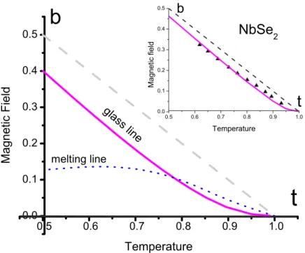
0 + 1 = 0, one obtainsFIG. 2. 共Color online兲 Phase diagram at high temperatures 共t=T/Tc⬎0.5兲. The static glass transition 共the magenta solid line兲, Eq. 共96兲, is
given for Gi = 1.25⫻10−5and n = 0.001. A
sche-matic behavior of the order-disorder transition is shown by a dashed line. It separates crystalline from homogeneous phases. Below the intersec-tion with the glass line, it is the “melting line,” while above it, it becomes a “peak effect line.” In the inset, we present the best fit for the irrevers-ibility line in NbSe2共see Ref. 36兲, with
4n03/2−
冉
aT0+ 403/2+ 01/2冊
+ 1 = 0, resulting in = 共2n兲1/3共aT g − aT兲 = − 共2n兲1/3⌬T. 共66兲The EA order parameter vanishes on the dynamical glass line and increases below it. In real space, the second term in Eq. 共65兲 corresponds to a constant 共the persistent component兲.20
The expression foris given by a solution of Eq.共53兲 with
0=共2n兲−2/3, 4n3/2− 4共2n兲−1/3 − aT
冉
1 − i 4ah冊
+ 1 = 0. 共67兲The regular component of the correlator in thespace, there-fore, decreases as a power C共兲⬀共/GL兲−1/2.
Having completed the solution of the gap equation, we now use it to calculate physical quantities other than the correlator.
IV. dc SUPERCURRENT A. LLL contribution
In the homogeneous phase, the current density after dis-order averaging is independent of bothand r. The average supercurrent density, therefore, is 共in the geometry consid-ered in this paper, the current flows in the y direction兲
jLLL⬅ JLLL J
⬘
= − i 2 共2兲3 VT冕
r具⌽r *共兲 +y⌽r共兲 −关y⌽r *共兲兴 +⌽r共兲典 = v冕
kz Ck z, 共68兲where具¯典 denotes both thermal and disorder averages, and J
⬘
=共2兲បe3*m*l t ␣l2 z= 2b1/2g 共8兲4J0 with J0= e* 冑2Gi 16Tc␥aប2 , using the
solu-tions of the gap equation and integrating over kz. In the liquid
and glass phases, the supercurrent is given by jLLL liq = 2
冉
8 g冊
1/3 0 1/2 v, 共69兲 jLLL glass = 2冉
8 g冊
1/3冋
1 共2n兲1/3+ aT g − aT 4册
v, 共70兲respectively. Here,0 is a solution to Eq.共50兲 given in Eq.
共51兲.
Therefore, within the LLL approximation, the supercur-rent is proportional to velocity times an expression analytic in velocity. Consequently, even at criticality, there exists fi-nite conductivity jLLL
liq
/v = 2
共
4ng兲
1/3, which is determined solely by disorder on the mesoscopic scale ng. The Ohmic behavior implies that there apparently is flux flow in both liquid and glass phases. On the glass transition, the LLL conductivity is continuous, although not a smooth function. In the glass state, we clearly see that there is no expectedvortex pinning and the conductivity is finite. On the liquid side, despite the critical divergencies in correlation function discussed in Sec. III C, the conductivity does not diverge, again in contrast to experiment. The only piece of physics that the LLL approximation is able to capture is the Bardeen-Stephen flux flow conductivity far from the glass transition line and the fluctuation conductivity in normal phase.18In the
clean limit32 共no disorder on the mesoscopic scale兲, n→0
with01/2= −aT
4 关see Eq. 共52兲兴 and one obtains
LLL=
JLLL
E =n
1 − t − b
b , 共71兲
where n is conductivity in the normal state. The full
for-mula provides a disorder correction.
As was mentioned in the Introduction, it is quite clear physically why the LLL approximation contains the Ohmic contribution only. The current generally is proportional to a gradient of the superfluid density, which, in turn, is propor-tional to the electric field. The pinning effects, therefore, ap-pear due to higher Landau levels only. We, therefore, gener-alize the discussion to the lowest states at which the pinning appears.
B. Higher Landau level contribution to current The argument above leading to an Ohmic dependence of the current on electric field in LLL共confirmed by the direct calculation in the previous section兲 is not valid already for the first LL, N = 1: the current is no longer a curl of the superfluid density. It is natural to assume that the HLL cor-rections to fields in Eq. 共22兲 can be considered as a
pertur-bation. Furthermore, to leading order in the perturbation, a nonzero contribution to current comes solely from the first LL共1LL兲: j = jLLL+ jHLL, jHLL= − i 2 共2兲3 VT
冕
r 具⌽r *共兲 +y⌰r共兲 −关y⌰r *共兲兴 +⌽r共兲 + c.c.典. 共72兲This is due to the fact that the operatorycontains just one,
raising or lowering the Landau number operator共in addition to a constant proportional to v兲. Thus one needs the wave function up to the first LL only,
⌿r共兲 = ⌽r共兲 + ⌰r共兲,
and considers it to first order in⌰r共兲.
In this section, we use a simplified model compared to that used in the derivation of the gap equation in the previous section. The difference consists in the application of the steepest descent approximation 共similar to that which was utilized and discussed in Sec. III B兲 already in the MSR ac-tion. As in Sec. III B, due to the Gaussian damping factor in quartic terms 关see Eq. 共24兲兴, we neglect all the terms
off-diagonal in momenta k both in the LLL and the HLL contri-butions:
Afree=
冕
k, 关⌽k, * Dk −1⌽ k,+⌰k, * D1k−1 ⌰k,兴, Adis= − rg 共2兲2␦␦k冕
k,关kz兴,, ␦k1z−k2z+k3z−k4z共⌽k,k1z, * x⌽k,k2z,兲 ⫻共⌽k,k* 3z,x⌽k,k4z,兲 + ⌬Adis, ⌬Adis= − 23/2iv rg 共2兲2␦␦k冕
k,关kz兴,, ␦k1z−k2z+k3z−k4z ⫻关共⌽k,k* 1z,x⌽k,k2z,兲共⌽k,k3z, * x⌰k,k4z,兲 − c.c.兴. 共73兲 Here, the inverse propagator for 1LL isD1k−1 =
冢
0 i⬘
2 + kz 2+ 2a h 1 − i⬘
2 + kz 2 + 2ah 1 − 1冣
, 共74兲 where ah 1= ah+ b is the large “mass” of the first LL
excita-tions. The coefficient in the disorder term is chosen in such a way that the LLL gap equation obtained from this action coincides with Eq. 共35兲. Physically, this assumption is
equivalent to replacing an approximate Landau degeneracy by an exact one. In addition, we ignore the interaction term since, as was noted in Sec. III C, the interaction effects can be accounted for by renormalization of the free part of LLL action, where ah is replaced by aint.
The correction term⌬Adis is already proportional to the
electric field via the factorv due to the fact that the integral of a product of three LLL Landau harmonics and one 1LL harmonic, Eq. 共19兲, vanishes at zero electric field. Since
Afreedoes not “mix” LLL with 1LL, the leading contribution
to jHLL, Eq.共72兲, will be of the second order in HLL ⌰ and
will come from all the connected diagrams proportional to ⌬Adis.
The HLL contribution to the current from the disorder part is jHLL= 2ng共1 + 2v2兲 共2兲2a h 1 v
冕
k关kz兴 ␦k1z−k2z+k3z−k4z具共⌽kk1z * x⌽kk2z兲 ⫻共⌽kk3z * ↑⌽kk2z兲典. 共75兲One, therefore, faces a problem of a consistent calculation of the four-point Green’s function. Diagrammatically, within the linear response theory, it was approximated by a resum-mation of the “diffusion” and “Cooperon” chains.1 We
cal-culate this function using a systematic approach by differen-tiating four times the Gaussian effective action defined in Sec. II.
Factorization of the action and of the current with respect to index k leads to proportionality of all physical quantities to the Landau degeneracy. Dropping below the index k and denoting kzsimply by k, one can express the HLL current as
jHLL=
2ng共1 + 2v2兲
共2兲2a h
1 vHLL, 共76兲
with the HLL contribution to the conductivity, HLL=
冕
兵prqs其 ␦p+q−r−q2x u1,v1 ↑ u2,v2具⌽ p *u1⌽ q *u2⌽ r v1⌽ s v2典 c, 共77兲 proportional to the connected part of the four-point correla-tion funccorrela-tion.C. Four-point correlators
The calculation of the four-point correlators is quite lengthy, so we first describe the general structure of the terms appearing in it. The gap equation derived in Sec. III B for Green’s function GAB=具⌽A⌽B
*典 共where indices A and B
de-note the full index set of the order parameter兲 can be gener-alized to include the rest of Green’s functions FAB=具⌽A⌽B典
and FAB *
=具⌽A *⌽
B
*典. In U共1兲 symmetric theories, like the one
we consider, the last propagators are identically equal to zero due to the symmetry. However, their functional derivatives do contribute to equations for the higher vertex functions and will be necessary for our discussion.
We write the generalized gap equations in a standard form30,31
冉
FB1A1 * GA1B1 GA1B1 * FB1A1冊
冢
冏
␦2A g关⌽¯ ,G兴 ␦⌽¯ A1 * ␦⌽¯ A2 *冏
Tr冏
␦2A g关⌽¯ ,G兴 ␦⌽¯ A1 * ␦⌽¯ A2冏
Tr冏
␦2A g关⌽¯ ,G兴 ␦⌽¯ A1␦⌽¯A2 *冏
Tr冏
␦2A g关⌽¯ ,G兴 ␦⌽¯ A1␦⌽¯A2冏
Tr冣
=␦B1A2, 共78兲where under the truncated part we understand functional de-rivatives of the Gaussian action AG关⌽¯ ,G兴, with propagators
G regarded as independent of the shift fields⌽¯ . Summation over repeated indices is assumed. The equations for a four-point vertex function are derived from Eq.共78兲 by
differen-tiating it twice with respect to the shift field ⌽¯ . The field dependence of the propagators, G关⌽¯ 兴 or F关⌽¯ 兴, determined by the gap equation共with external “source” present兲, should be taken into account. It provides the “chain” parts propor-tional to ␦G
␦⌽¯, ␦F
␦⌽¯, ␦2G
␦⌽¯␦⌽¯ , . . .. From the U共1兲 symmetry, one can
infer that there are two nontrivial vertex contributions: the diffuson and the Cooperon parts defined by the ␦G
␦⌽¯␦⌽¯* and
␦F
␦⌽¯␦⌽¯ second derivatives, respectively.
The diffusion and the Cooperon equations can be obtained from Eq.共78兲, differentiating its 共11兲 component with respect
to⌽¯C2 and⌽¯C1 *
and differentiating the共21兲 component with