Nano-roughness measurements with a modified Linnik microscope and the uses of full-field heterodyne interferometry

(1)

Nano-roughness measurements with a modified

Linnik microscope and the uses of full-field

heterodyne interferometry

Yen-Liang Chen Zhi-Cheng Jian Hung-Chih Hsieh Wang-Tsung Wu

Der-Chin Su,MEMBER SPIE National Chiao Tung University

Department of Photonics and Institute of Electro-Optical Engineering

1001 Ta-Hsueh Road Hsin-Chu 30050, Taiwan

E-mail: [email protected]

Abstract. A collimated heterodyne light enters a modified Linnik micro-scope, and the full-field interference signals are taken by a fast CMOS camera. The sampling intensities recorded at each pixel are fitted to derive a sinusoidal signal, and its phase can be obtained. Next, the 2-D phase unwrapping technique is applied to derive the 2-D phase tion. Then, Ingelstam’s formula is used to calculate the height distribu-tion. Last, the height distribution is filtered with the Gaussian filter, the roughness topography and its average roughness can be obtained and its validity is demonstrated. © 2008 Society of Photo-Optical Instrumentation Engineers. 关DOI: 10.1117/1.3050357兴

Subject terms: roughness measurement; heterodyne interferometry; Linnik microscope; interference microscopy.

Paper 080524R received Jul. 3, 2008; revised manuscript received Nov. 4, 2008; accepted for publication Nov. 5, 2008; published online Dec. 22, 2008.

1 Introduction

The surface quality of optical and microelectronic compo-nents is very important for many manufacturing processes. The conventional stylus method is often used for surface roughness measurements. However, it has certain limita-tions. Among these, the stylus can potentially deform or damage the sample surface. In addition, the stylus travels slowly, so the measurement process is time consuming. To overcome these drawbacks, several nondestructive optical methods1–7 have been proposed and have good measure-ment results. In this paper, an alternative method for mea-suring surface roughness with heterodyne interference mi-croscopy is presented. The light beam coming from a heterodyne light source is collimated and enters a modified Linnik microscope, and the full-field interference signals are taken by a fast CMOS camera. Each pixel records a series of the sampling intensities of a sinusoidal signal. These sampling intensities are fitted8to derive the associ-ated sinusoidal signal, and the phase of that pixel can be obtained. Then, the phase of any pixel can be obtained similarly. Next, the 2-D phase distribution can be deter-mined with the 2-D phase unwrapping technique.9 The height distribution can be derived with the data of the 2-D phase distribution and Ingelstam’s formula.10Last, the data of the height distribution is filtered with the Gaussian filter defined by ISO 11562共Ref. 11兲, and the roughness topog-raphy and its average roughness can be obtained. A rough-ness standard is tested to show the validity of this method. This method has some merits, such as simple optical con-figuration, high measurement accuracy, and rapid measure-ment.

2 Principle

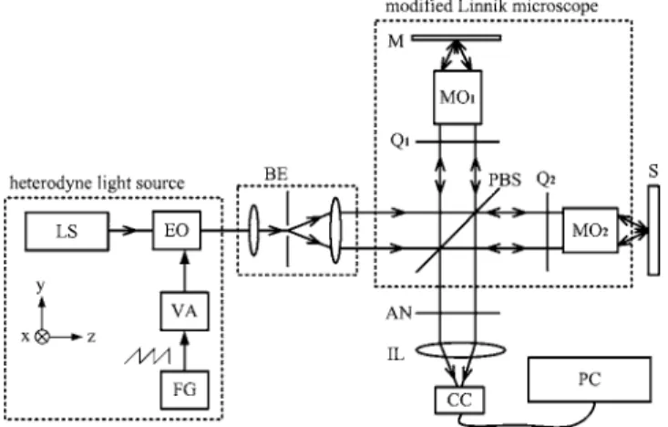
Figure 1 shows a schematic diagram of this method. For

convenience, the +z axis is chosen to be along the light propagation direction, and the y axis is along the vertical direction. A light coming from a heterodyne light source12 has a frequency difference f between the s- and the p-polarizations, and its Jones vector can be written as

E =

_冑

1

2

冋

exp共i␲ft兲

exp共− i␲ft兲

册

. 共1兲

The light beam is expanded and collimated by a beam ex-pander BE. It enters a modified Linnik microscope, which consists of a polarization beamsplitter PBS, a reference mirror M, two quarter-wave plates Q1and Q2with the fast axes at 45 deg with respect to the x axis, and two identical microscopic objectives MO1 and MO2. In addition, a test

Fig. 1 Schematic diagram of this method. LS: laser light source;

EO: electro-optic modulator; FG: function generator; VA: voltage amplifier; BE: beam expander; PBS: polarizing beamsplitter; Q: quarter-wave plate; MO: microscopic objective; M: mirror; S: sample; AN: analyzer; IL: imaging lens; CC: CMOS camera; and PC: personal computer.

(2)

sample S, an analyzer AN with the transmission axis at 45 deg with respect to the x axis, an imaging lens IL, and a CMOS camera CC are introduced into the optical configu-ration, which is also a modified Twyman-Greeen interfer-ometer. In this interferometer, the paths of two collimated beams are 共1兲 PBS→Q1→MO₁→M→MO₁→Q₁→PBS

→AN→IL→CC 共the reference beam兲, and 共2兲 PBS

exp

冉

i␲

冉

ft + 4d ␭

冊冊

, 共3兲

where TPBS and RPBS are the transmission matrix and the reflection matrix of the PBS, rm and rs are the reflection coefficients of the M and the S, respectively; and 2d is the optical path difference between these two beams. Thus, the interference signals measured by the CC can be written as

I =兩Er+ Et兩2= I0+␥· cos共2␲ft +␾0兲 = A · cos共2␲ft兲

+ B · sin共2␲ft兲 + C, 共4兲

where I0 is the mean intensity;␥ and␾0 are the visibility and the phase, respectively, of the interference signal; and

A, B, and C are real numbers. Moreover, ␾0 equals the phase difference between Erand Et. These values are

I0= 1 16共rm 2 + rs 2_兲, _共5兲 ␥=− rmrs 8 , 共6兲 and ␾0共x,y兲 =4␲d ␭ =␾1+␾2= 2n␲+␾2= 2n␲+ tan−1

冉

− B A

冊

, 共7兲 where␾1is the phase of the reference point on the S. This equals 2n␲, where n is an integer, and can be omitted.␾2is the relative phase with respect to the reference point, and it depends on the height distribution h共x,y兲 of the sample surface.

. 共9兲

Equation共8兲can be rewritten as

冢

A B C

冣

=共MtM兲−1Mt

冢

I1 I2 : In

冣

, 共10兲

where Mtmeans the transpose matrix of M. Equation共10兲 can be solved by using the least-square fitting algorithm on IEEE Standards,8and the data of A and B can be obtained. These are substituted into Eq.共7兲, and the data of␾₂can be derived. If these processes are applied to all other pixels, then the associated data␾2共x,y兲 can be obtained similarly. Except the intrinsic electronic noises, the data␾2共x,y兲 are easily influenced by the ambient motions because of the two-path optical configuration. To reduce the phase outliers and dropouts that often occur near groove edges, ␾2共x,y兲 are processed with the special algorithm for noisy phase-map processing.13 In addition, the 2-D phase unwrapping technique9is applied to solve the phase ambiguity, and the full-field phase distribution ␾共x,y兲 is obtained. In this method, the light beam is converged to incident on the S by using the MO2with numerical aperture NA, so the relation between␾共x,y兲 and the height distribution h共x,y兲 of the S can be expressed as

h共x,y兲 =␭ ·␾共x,y兲

4␲ · k, 共11兲

(3)

k = 1 +NA

2

4 , 共12兲

according to Ingelstam’s formula.10 If the derived data of ␾共x,y兲 and the value of k obtained from Eq.共12兲are sub-stituted into Eq.共11兲, then h共x,y兲 can be calculated.

Last, the Gaussian filter defined by ISO 11562共Ref.11兲 is then applied to subtract the waviness part of h共x,y兲, and the roughness part R共x,y兲 can be obtained. Based on the formula of 2-D roughness parameter defined by the ISO 25178-2 standard,14 the average roughness value Sa is de-fined as Sa= 1 UV

兺

_k=0 U−1

兺

l=0 V−1 兩R共xk,yl兲 −␮兩, 共13兲

where U⫻V are the pixel numbers of one frame, and␮is the average of R共x,y兲. Substituting the data of R共x,y兲 and ␮into Eq.共13兲, the data of Sacan be obtained.

3 Experiments and Results

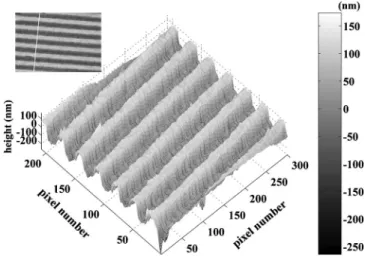
To demonstrate the validity of this method, we tested a roughness standard specimen with rectangular wave forms, as shown in Fig.2. The pitch of the rectangular wave forms is 20␮m. It was also measured with a commercial stylus instrument by the National Measurement Laboratory in Tai-wan, and its average roughness value is 67 nm. An He-Ne laser with 632.8-nm wavelength, two 10⫻ microscopic ob-jectives with NA= 0.25, and a CMOS camera 共Basler/ A504K兲 with 8-bit gray levels and 300⫻210 pixels were used in this test. Under the conditions f = 20 Hz and fc = 300.3 frames/s, 300 frames were taken in 1 s. A least-squares sine fitting algorithm on the IEEE 1241 standard in a MATLAB program was utilized, and the data of␾2共x,y兲 were obtained and are shown in Fig. 3. Then, the data of

␾2共x,y兲 were processed with the 2-D phase unwrapping technique, and the full-field phase distribution␾共x,y兲 were obtained and are shown in gray levels in Fig.4. In addition, the data of ␾共x,y兲 were substituted into Eq. 共11兲 and the data of h共x,y兲 were calculated. Last, the data of h共x,y兲 were filtered by a bandpass Gaussian filter with the long cutoff wavelength ␭c= 80␮m to reduce the waviness and the short cutoff wavelength ␭s= 2.5␮m to eliminate the noise.15,16 The full-field surface roughness topography

R共x,y兲 is shown in gray levels in Fig.5; its average rough-ness can be calculated with Eq. 共13兲 and obtained as Sa = 65.7 nm.

4 Discussion

The profile along the white line in the inset in Fig.5 was also measured by the contact stylus instrument. Their mea-sured results are shown together in Fig.6for comparison: the solid curve is for this method, and the dotted curve is for the contact stylus instrument. From Fig. 6, it can be obtained that their cross-correlation function17 is up to 91.5%. Because the total points with different measured results are less than 10%, both are acceptable.18

The phase distribution␾共x,y兲 is the relative data and is shifted as the optical configuration is rearranged. Despite the shift of ␾共x,y兲, the measured results R共x,y兲 have the same profile with a different value of ␮. The data of Sais Fig. 2 The test sample, which is a roughness standard specimen

with rectangular wave forms.

Fig. 3 The full-field phase distribution␾2共x,y兲 in gray levels.

Fig. 4 The full-field phase distribution␾共x,y兲 in gray levels.

Fig. 5 The measured full-field roughness topography R共x,y兲 in gray

(4)

still unchanged. After filtering by the Gaussian filter, the surface waviness and the alignment error can be subtracted. The errors in this technique may be influenced by the fol-lowing factors:

• Sampling error. This depends on the frequency of the heterodyne interference signal, the camera recording time, the frame period, the frame exposure time, and the number of gray levels. The condition fc = 300.3 frames/s is chosen based on the optimal con-dition proposed by Jian et al.19 to decrease the mea-surement error, and the sampling error ⌬␾s is about 0.036 deg.

• Polarization-mixing error. Owing to the extinction ratio effect of a polarizer, mixing of light polarization occurs. In our experiments, the extinction ratio of the polarizer 共Japan Sigma Koki, Ltd.兲 is 1⫻10−5. This can be estimated in advance to modify the measured results, and the polarization-mixing error can be de-creased to ⌬␾p= 0.03 deg with this modification.20 Consequently, the theoretical error of this method is ⌬Sa=⌬h =

␭

4␲k共⌬␾s+⌬␾p兲 = 0.06 nm. 共14兲 Hence, this method has better theoretical resolution than that of phase-shifting interferometry and white-light interferometry.21

5 Conclusion

In this paper, an alternative method for measuring full-field surface roughness has been proposed by introducing het-erodyne interfermoetry into a modified Linnik microscope. The full-field interference signals are taken by a fast CMOS camera, and a series of the sample intensities of a sinu-soidal signal are recorded at each pixel. The associated phase of each pixel can be derived with a least-squares sine fitting algorithm. The height distribution can be derived

with the 2-D phase unwrapping technique and Ingelstam’s formula. Last, the data of height distribution is filtered, and the roughness topography and its average roughness can be obtained. The method’s validity has been demonstrated, and it has some merits, such as simple optical configura-tion, high measurement accuracy, and rapid measurement.

Acknowledgments

This study was supported in part by the National Science Council, Taiwan, under Contract No. NSC95-2221-E009-236-MY3.

References

1. J. M. Bennett, “Recent developments in surface roughness character-ization,”Meas. Sci. Technol.3, 1119–1127共1992兲.

2. U. Persson, “Real time measurement of surface roughness on ground surface using speckle-contrast technique,” Opt. Lasers Eng. 17, 61–67共1992兲.

3. R. Windecker and H. J. Tiziani, “Optical roughness measurements using extended white-light interferometry,”Opt. Eng.38, 1081–1087

共1999兲.

4. S. H. Wang, C. Quan, C. J. Tay, and H. M. Shang, “Surface rough-ness measurement in the submicrometer range using laser scattering,”

Opt. Eng.39, 1597–1601共2000兲.

5. C. Cheng, C. Liu, N. Zhang, T. Jia, R. Li, and Z. Xu, “Absolute measurement of roughness and lateral-correlation length of random surfaces by use of the simplified model of image-speckle contrast,”

Appl. Opt.41, 4148–4156共2002兲.

6. A. Duparre, J. F. Borrull, S. Gliech, G. Notni, J. Steinert, and J. M. Bennett, “Surface characterization techniques for determining the root-mean-square roughness and power spectral densities of optical components,”Appl. Opt.41, 154–171共2002兲.

7. I. Yamaguchi, K. Kobayashi, and L. Yaroslavsky, “Measurement of surface roughness by speckle correlation,”Opt. Eng.43, 2753–2761

共2004兲.

8. IEEE, “Standard for terminology and test methods for analog-to-digital converters,” IEEE Std. 1241–2000, pp. 25–29共2000兲. 9. D. C. Ghiglia and M. D. Pritt, “Two-dimensional phase unwrapping:

theory, algorithms, and software,” Wiley, New York共1998兲. 10. E. Ingelstam, “Problems related to the accurate interpretation of

mi-crointerferograms,” Interferometry, National Physical Laboratory Symposium 11, 41–163共1960兲.

11. “Geometrical product specifications共GPS兲—surface texture: profile method—metrological characteristics of phase correct filters,” ISO 11562共1996兲.

12. D. C. Su, M. H. Chiu, and C. D. Chen, “Simple two frequency laser,”

Precis. Eng.18, 161–163共1996兲.

13. J. A. Quiroga and E. Bernabeu, “Phase-unwrapping algorithm for noisy phase-map processing,” Appl. Opt. 33, 6725–6731共1994兲. 14. “Geometrical product specifications共GPS兲—surface texture: areal—

part 2: terms, definitions, and surface texture parameters,” ISO/DIS 25178-2共2008兲.

15. “Geometrical product specifications共GPS兲—surface texture: profile method—rules and procedures for the assessment of surface texture,” ISO 4288共1996兲.

16. “Geometrical product specifications共GPS兲—surface texture: profile method—nominal characteristics of contact 共stylus兲 instruments,” ISO 3274共1996兲.

17. J. Song, T. Vorburger, T. Renegar, H. Rhee, A. Zheng, L. Ma, J. Libert, S. Ballou, B. Bachrach, and K. Bogart, “Correlation of topog-raphy measurements of NIST SRM 2460 standard bullets by four techniques,” Meas. Sci. Technol. 17, 500–503共2006兲.

18. R. Krüger-Sehm and J. A. Luna Perez, “Proposal for a guideline to calibrate interference microscopes for use in roughness measure-ments,” Int. J. Mach. Tools Manuf. 41, 2123–2137共2001兲. 19. Z. C. Jian, Y. L. Chen, H. C. Hsieh, P. J. Hsieh, and D. C. Su,

“Optimal condition for full-field heterodyne interferometry,” Opt. Eng.46, 115604共2007兲.

20. M. H. Chiu, J. Y. Lee, and D. C. Su, “Complex refractive-index measurement based on Fresnel’s equations and uses of heterodyne interferometry,”Appl. Opt.38, 4047–4052共1999兲.

21. H. G. Rhee, T. V. Vorburger, J. W. Lee, and J. Fu, “Discrepancies between roughness measurements obtained with phase-shifting and white-light interferometry,”Appl. Opt.44, 5919–5927共2005兲. Fig. 6 Measured profiles along the white line in the inset in Fig.5

with this method共solid curve兲 and the contact stylus instrument 共dot-ted curve兲.

(5)

Yen-Liang Chen received his MS degree

from the Department of Atomic Science, Na-tional Tsing Hua University, Taiwan, in 2000 and is now working toward his PhD degree in optical metrology at the Institute of Electro-Optical Engineering of National Chiao Tung University. His current research activities are in optical metrology.

Zhi-Cheng Jian received his MS degree

from the Institute of Electro-Optical Engi-neering, National Taipei University of Tech-nology, Taiwan, in 2002 and is now working toward a PhD degree in optical metrology at the Institute of Electro-Optical Engineering of National Chiao Tung University. His cur-rent research activities are in optical metrol-ogy.

Hung-Chih Hsieh received his MS degree

from the Institute of Electro-Optical Engi-neering, National Chiao Tung University, Taiwan, in 2005 and is now working toward his PhD degree in optical metrology at the Institute of Electro-Optical Engineering of National Chiao Tung University. His current research activities are in optical metrology and nondestructive testing.

Wang-Tsung Wu received his BS degree in

physics from the National Tsing Hua Univer-sity, Taiwan, in 2006 and is now working to-ward his PhD degree in optical metrology at the Institute of Electro-Optical Engineering of National Chiao Tung University. His cur-rent research activities are in optical metrol-ogy and nondestructive testing.

Der-Chin Su received his BS degree in

physics from the National Taiwan Normal University in 1975 and his MS and PhD de-grees in information processing from the To-kyo Institute of Technology in 1983 and 1986, respectively. He joined the faculty of the National Chiao Tung University in 1986, where he is currently a professor with the Institute of Electro-Optical Engineering. His current research interests are in optical test-ing and holography.