A multiobjective hybrid genetic algorithm for the capacitated multipoint network design problem

(1)

A Multiobjective Hybrid Genetic Algorithm for the

Capacitated Multipoint Network Design Problem

Chi-Chun Lo, Member, IEEE, and Wei-Hsin Chang, Member, IEEE

Abstract—The capacitated multipoint network design problem (CMNDP) is NP-complete. In this paper, a hybrid genetic algo-rithm for CMNDP is proposed. The multiobjective hybrid genetic algorithm (MOHGA) differs from other genetic algorithms (GA’s) mainly in its selection procedure. The concept of subpopulation is used in MOHGA. Four subpopulations are generated according to the elitism reservation strategy, the shifting Prüfer vector, the stochastic universal sampling, and the complete random method, respectively. Mixing these four subpopulations produces the next generation population. The MOHGA can effectively search the fea-sible solution space due to population diversity. The MOHGA has been applied to CMNDP. By examining computational and analyt-ical results, we notice that the MOHGA can find most nondomi-nated solutions and is much more effective and efficient than other multiobjective GA’s.

Index Terms—Genetic algorithms, minimal spanning tree, mul-tiobjective function, nondominated solution, subpopulation.

I. INTRODUCTION

T

HE problem of effectively transmitting data in a network involves the design of communication subnetworks. A critical issue in network design is to find a set of links which connect communication nodes such that the cost (or delay) of the selected paths between pairs of nodes is minimized, and the constraints of network capacity and reliability are met. In the real world, network design has long been recognized as multiobjective in nature. For a centralized multipoint network; i.e., a tree network, the network design problem gives rise to a well-known combinatorial optimization problem, namely, the constrained minimal spanning tree (CMST) problem. The CMST is NP-complete. Many heuristics, e.g., [3], [5], [10], [11], [14], [16], [30], have been proposed. However, their works took account of only cost or delay. In recent years, ge-netic algorithms (GA’s) have been applied to various multiple criteria decision making (MCDM) problems. Fonseca and Fleming [12] explored the fitness assignment method. Horn et al. [22] investigated multiobjective problems via test functions. Tamaki et al.. [35] studied the multiobjective scheduling problem and the decision tree induction problem. Schaffer [33] proposed the vector evaluated genetic algorithm (VEGA) to solve multiobjective optimization problems. In VEGA, a population is divided into many disjoint subpopulations. For each subpopulation, a different objective function is used to

Manuscript received February 17, 1999; revised February 29, 2000. This paper was recommended by Associate Editor Y. Y. Haimes.

The authors are with Institute of Information Management, Na-tional Chiao-Tung University, Hsinchu 300, Taiwan, R.O.C. (e-mail: cclo@cc.nctu.edu.tw).

Publisher Item Identifier S 1083-4419(00)04124-8.

evaluate the fitness of chromosomes (solutions). Ishibuchi and Murata [24] presented the single-objective genetic algorithm (SOGA) that translates multiple objective functions into a single-objective function by using weighting functions.

In this paper, the capacitated multipoint network design problem (CMNDP) is considered. A multiobjective hybrid genetic algorithm (MOHGA) is proposed for CMNDP. The MOHGA differs from other GA’s mainly in its selection procedure. The concept of subpopulation is used in MOHGA. Four subpopulations are generated according to the elitism reservation strategy, the shifting Prüfer vector, the stochastic universal sampling, and the complete random method, respec-tively. Mixing these four subpopulations produces the next generation population. The MOHGA can effectively search the feasible solution space due to population diversity. By applying MOHGA to CMNDP, we notice that the MOHGA can find most nondominated solutions in the feasible solution space and is much more effective and efficient than other multiobjective GA’s.

In the next section, a brief introduction to GA’s is given. Sec-tion III describes the MOHGA. The problem formulaSec-tion of CMNDP is detailed in Section IV. In Section V, computational experiments are presented. Section VI concludes this paper with possible future research directions.

II. GENETICALGORITHMS

A. Overview

The concept of a GA, introduced by Holland [21], is based on the mechanics of natural selection and natural genetics. A GA starts with an initial set of random solutions, called a

pop-ulation. Each individual in the population is called a chromo-some, representing a solution to the problem. The initial

popula-tion evolves through successive iterapopula-tions, called generapopula-tions. A measure of fitness defines the quality of an individual chro-mosome. In each generation, chromosomes are evaluated by a fitness function, also called an evaluation function. After a number of generations, highly fit individuals, which are anal-ogous to good solutions to a given problem, will emerge. Be-cause of this property, the GA is more robust than existing direct search methods, like the hill climbing method [27].

A GA consists of five components, as described in Davis’s book [7]. These five components are as follows:

1) a method for encoding potential solutions into chromo-somes;

2) a means of creating the initial population;

(2)

3) an evaluation function that can evaluate the fitness of chromosomes;

4) genetic operators that can create the next generation pop-ulation;

5) a way to set up control parameters; e.g., population size, the probability of applying a genetic operator, etc. B. Encoding Methods

To solve a problem using GA, the method of encoding its so-lutions is very important. For a CMST problem, its tree repre-sentation is encoded. There are three ways of encoding tree: 1) edge encoding [15], 2) vertex encoding [15], and 3) edge-and-vertex encoding [30].

1) Edge Encoding: Consider an undirected and connected graph , where is the set of vertices of , and

is the set of edges of . For each edge of , an index

is assigned; i.e., , where is the

number of edges of . tree of can be represented by

edge encoding, where if is an edge of

and 0 otherwise. Edge encoding is an intuitive representation of a tree. In a complete graph of nodes, the total number of edges

is equal to . There are possible values

for . All trees have exactly edges. If contains other than 1s, it is not a tree. However, even if contains exactly 1s, it is still unlikely that represents a tree. Therefore, edge encoding is not suitable for CMST due to the extremely low probability of using it to obtain a tree.

2) Vertex Encoding: In 1889, Cayley [4] proved the fol-lowing formula: the number of spanning trees in a complete graph of nodes is equal to . Prüfer [32] presented the simplest proof of Cayley’s formula by establishing a one-to-one correspondence between the set of spanning trees and a set of sequences of integers, with each integer between 1 and inclusive [15]. The sequence of integers for encoding a tree is known as Prüfer vector (or Prüfer number). The Prüfer encoding and decoding procedures are explained as follows:

Prüfer encoding procedure

For a tree , its corresponding Prüfer vector can be ob-tained by the following steps:

Step 1) Let vertex be the lowest labeled leaf node (node of degree 1) of ; let vertex be incident to vertex ; append to the end of ( is constructed from left to right in sequence).

Step 2) Remove vertex and the edge , which connects vertices and .

Step 3) Go back to Step 1 until there is only one edge left in is obtained.

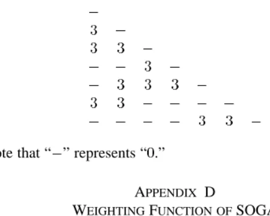
For example, Fig. 1 depicts a 7-node tree. Vertex 2 is the lowest labeled leaf node and vertex 1 is incident to vertex 2. Vertex 1 becomes the first element of ; then, vertex 2 and edge are removed. In the second iteration, vertex 3 is the lowest leaf node and vertex 1 is incident to vertex 3. Append vertex 1 to , and then remove vertex 3 and edge . Repeat the process until only edge is left. is obtained and is equal to .

Prüfer decoding procedure

For a Prüfer vector and the set of its eligible vertices , a unique tree representation of , denoted as , can be obtained

Fig. 1. Seven-node tree and its Prüfer encoding= [1; 1; 4; 4; 4].

by the following steps.

Step 1) Let vertex be the lowest eligible node of and vertex be the first element of . If , add the edge from to into , and then remove vertex from and vertex from .

Step 2) Repeat Step 1 until no elements are left in . Step 3) For the remaining last two vertices and of ,

add the edge from to into .

3) Edge-and-Vertex Encoding: Palmer and Kershenbaum [30] proposed the link-and-node biased encoding method, also termed as the edge-and-vertex encoding as presented by Gen and Cheng [15]. This encoding does not directly encode a tree, but a modified cost matrix. Based on the modified cost matrix, a tree is generated by Prim’s algorithm [31]. For a graph of nodes, the chromosome of this representation has biases, including node bias and link bias , for the nodes and each of the links, for a total of

biases. In this method, two parameters, and , are used as the multipliers of the maximum link cost, . The cost

matrix is biased by , and using

Palmer claimed that this version of representation could encode any tree, given appropriate values of the , and [30]. However, as pointed out by Gen and Cheng [15], this encoding has three major disadvantages:

1) it requires a very long encoding (memory cost);

2) it needs a conventional minimum spanning tree algorithm to generate a tree from its encoding (computation cost); 3) it contains no useful information such as degree,

connec-tion, etc, about a tree.

III. MULTIOBJECTIVEHYBRIDGENETICALGORITHM

For a multiobjective optimization problem, its nondominated solutions (The definition is stated in Appendix A.) can be found by GA’s. To find good solutions via GA’s, the concept of sub-population proposed by Schaffer [33] is a promising approach. A. Subpopulation

1) Elitism Reservation Strategy: In traditional GA’s, a chro-mosome in the current generation is selected into the next gen-eration with certain probability. The best chromosomes of the current generation may be lost due to mutation, crossover, or selection during the evolving process, and subsequently causes

(3)

difficulty in reaching convergence. In other word, it takes more generations; i.e., running time, to get quality solutions. Tamaki et al.. [35] proposed an elitism reservation strategy that permits chromosomes with the best fitness to survive and be carried into the next generation.

2) Shifting Prüfer Vector: The shifting Prüfer vector, introduced in this paper, is a genetic operator. The well-known problem of Prüfer encoding [30] is that it does not preserve locality. Changing one element of a Prüfer vector can change its corresponding tree topology dramatically. To remedy this problem, we introduce a new genetic operator, called the shifting Prüfer vector. This operator maintains maximum locality; i.e., it keeps the similarity between chromosomes. The concept of the shifting Prüfer vector is stated as follows: it replaces the leftmost element of a Prüfer vector by a randomly selected nonleftmost element of the same vector. The new vector differs from the old one only in the leftmost element. Thus, the new topology differs from the old one in at most two edges (The proof of this assertion is presented in Appendix B.) In most cases, the difference is only one edge. The shifting Prüfer vector is a local search method. According to the results obtained by the well-known Add and Drop searching heuristics [26], [28], [31], changing only one element in every iteration of the search process always leads to a globally optimal solution. Thus, the shifting Prüfer vector can significantly improve the quality of newly found chromosomes.

Fig. 2 illustrates the new tree after the shifting Prüfer vector is applied to the 7-node tree shown in Fig. 1. We notice that the new tree and the old one differ in only one edge.

3) Stochastic Universal Sampling: A simple way to per-form sampling is to spin a roulette wheel. Unfortunately, this sampling method does not guarantee that any particular sample will actually be chosen in any given generation. This is a well-known problem of the roulette wheel selection method. Baker suggested the stochastic universal sampling method [2]. Baker’s algorithm completes the whole sampling in a single pass, and requires only one random number. A wheel spin, whose size is equal to the population size, is divided into a number of equally spaced markers. A single spin is used to generate the random number. The expected value for

chromosome is expressed as , where

pop size represents population size and represents selection probability.

4) Complete Random Method: Population is generated ac-cording to random number and random position. The major reason for using the complete random method is to maintain the diversity of the population.

B. Mix Method

There are two competing factors in the selection procedure of a genetic search. They are selection pressure and population diversity. An increase of selection pressure decreases the diver-sity of the population, and vice versa [27]. The stochastic uni-versal sampling method increases selection pressure; however, it may cause the premature convergence of a genetic search. To decrease selection pressure, the complete random method

Fig. 2. New tree after applying the shifting Prüfer vector and its Prüfer encoding= [4; 1; 4; 4; 4].

can be used in conjunction with the stochastic universal sam-pling method. Nevertheless, the best chromosomes of the cur-rent generation may be lost due to crossover and mutation. This problem can be overcome by including the elitism reservation strategy during a genetic search. But, globally optimal solu-tions are rarely obtained. In order to find globally optimal so-lutions, the shifting Prüfer vector is added to the selection cedure. According to the discussions aforementioned, we pro-pose the mix method as follows: first, four subpopulations are generated according to the elitism reservation strategy [35], the shifting Prüfer vector, the stochastic universal sampling [2], and the complete random method, respectively; then, mixing these four subpopulations produces the next generation population. C. The Multiobjective Hybrid Genetic Algorithm

MOHGA

Step 1) Set the maximum number of generation, , and initialize the loop counter, , to zero.

Step 2) Produce the initial population, , by using the complete random method and Prüfer encoding. Step 3) Evaluate ; exit, if the solutions are found. Step 4) Generate the subpopulation, , by using the

elitism reservation strategy.

Step 5) Generate the subpopulation, , by using the shifting Prüfer vector.

Step 6) Generate the subpopulation, , by using the stochastic universal sampling with crossover prob-ability and mutation probability .

Step 7) Generate the subpopulation, , by using the complete random method.

Step 8) Form the next generation population, , by

mixing , and .

Step 9) Increase by 1; if is less than , then go to Step 3; otherwise, evaluate , exit.

where represents the probability of crossover, the prob-ability of mutation, the population of the -th generation, and the -th subpopulation of the -th generation.

IV. CAPACITATEDMULTIPOINTNETWORKDESIGNPROBLEM

A. Problem Formulation

The CMNDP can be formulated as follows:

(1)

(4)

subject to (3) (4) (5) (6) where

number of nodes in the network; set of links in the network;

-th link; and it may not exist for some ; given weight matrix;

weight of the -th node; spanning tree;

number of edges of ;

cost of connecting node to node ; i.e., the cost of link ; the cost matrix is symmetric;

average delay on link ; the delay matrix is symmetric;

the 0/1 decision variable; 1, if link is selected, and 0, otherwise.

Equation (3) guarantees that the total link weight does not ex-ceed the upper limit, (4) guarantees that the set of chosen links does not form any cycle, and (5) guarantees that enough links will be chosen to connect the network.

B. Applying MOHGA to CMNDP

1) Encoding Method: Prüfer encoding provides a one-to-one mapping between the set of spanning trees and the set of sequences of -integers [15], [30]. Because of this excellent property, we choose Prüfer encoding for encoding chromosomes.

2) Initial Population: Each individual chromosome in the initial population is a solution to the problem. We use the com-plete random method to generate the initial population.

3) Evaluation Function: We choose both link cost and trans-mission delay as the evaluation functions for CMNDP.

V. COMPUTATIONALEXPERIMENTS

A. Test Problems and Results

The simulator is coded in the C++ language and is running on an Intel Pentium-166 MHz PC with 64 MB RAM. In order to evaluate the solutions of CMNDP obtained by MOHGA, we examine a set of problems, with 7, 14, 28, and 56 nodes, re-spectively. The number of nondominated solutions obtained by MOHGA is affected by control parameters; e.g., mutation prob-ability, crossover probprob-ability, and the maximum number of gen-erations. The best solution in terms of cost , the best so-lution in terms of delay , or other solutions in terms of network designer’s preference can be deduced from all nondom-inated solutions. The maximum number of generations is depen-dent on problem size. The lager the problem size, the larger the feasible solution space. In other words, more generations are needed to find the solutions.

TABLE I

CPU TIME AND NUMBER OFSOLUTIONS OF THE7-NODEPROBLEMw.r.t. MOHGA, SOGA,ANDVEGA

Problem 1: For the 7-node network, nodes are randomly distributed. Control parameters are given as follows: mutation probability is set to 0.9, crossover probability is set to 0.5, population size is set to 100, and the maximum number of generations is set to 200. Cost, delay, and constrained weight matrices are given in Appendix C.

All the nondominated solutions; i.e., all possible spanning trees, are enumerated. By doing this, we are able to compare the quality of the solutions obtained by MOHGA directly with the enumerated solutions. The pair (total cost, total delay) represents a solution. By enumerating the solutions, we found all six nondominated solutions of this problem, which are

, and .

With ten runs, nondominated solutions obtained by MOHGA can be summarized as follows:

Set 1: Set 2:

Set 3: .

Sets 1, 2, and 3 are obtained 4, 4, and 2 times, respectively. Therefore, we can claim that the MOHGA finds 90% of all non-dominated solutions.

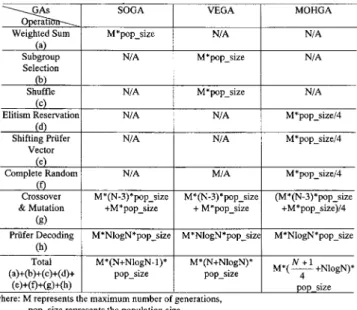
For comparison, the VEGA and the SOGA are applied to the same test problem. In the weighting function of SOGA, weights (cost) and (delay) are both set to 0.5 [24]. Note that we only consider the case in which and are both equal to 0.5, since the largest number of nondominated solutions are ob-tained by setting (Appendix D.) Other control parameters are set to the same value as those of MOHGA. Com-putational results are summarized in Table I.

Problem 2: A network of 14 nodes is considered in Problem 2. Network nodes are randomly distributed. Weight, cost, and delay are randomly generated. Control parameters are given as follows: mutation probability is set to 0.9, crossover probability is set to 0.4, population size is set to 100, and the maximum number of generations is set to 1000. Computational results are presented in Table II.

Problem 3: A network of 28 nodes is considered in Problem 3. Network nodes are randomly distributed. Weight, cost, and delay are randomly generated. Control parameters are given as follows: mutation probability is set to 0.99, crossover proba-bility is set to 0.4, population size is set to 100, and the maximum number of generations is set to1000. Computational results are shown in Table III.

Problem 4: A network of 56 nodes is considered in Problem 4. Network nodes are randomly distributed. Weight, cost, and delay are randomly generated. Control parameters are given as follows: mutation probability is set to 0.99, crossover proba-bility is set to 0.4, population size is set to 100, and the maximum

(5)

TABLE II

CPU TIME ANDNUMBER OFSOLUTIONS OF THE14-NODEPROBLEMw.r.t. MOHGA, SOGA,ANDVEGA

TABLE III

TABLE IV

number of generations is set to 10 000. Computation results are listed in Table IV.

Problems 5, 6, and 7: A network of 56 nodes is considered in Problems 5, 6, and 7. Network nodes are not randomly distributed. For Problem 5, most nodes reside at the upper left corner of the network. For Problem 6, node distribution is sparse. For Problem 7, node distribution is dense. Weight, cost, and delay are randomly generated. Control parameters are given as follows: mutation probability is set to 0.99, crossover probability is set to 0.4, population size is set to 100, and the maximum number of generations is set to 10 000. Computation results are reported in Tables V–VII.

Problem 8: Problem 8 is designed to evaluate the correct-ness of the mix method as described in Section III. Four algo-rithms are evaluated. In Algorithm 1, only the stochastic uni-versal sampling method is used in the selection procedure. Al-gorithm 2 is obtained by adding the complete random method to Algorithm 1. Algorithm 3 is obtained by adding the elitism reservation strategy to Algorithm 2. Algorithm 4 (the MOHGA) is obtained by adding the shifting Prüfer vector to Algorithm 3. Network nodes of 7, 14, and 28 are considered. Simulation re-sults are reported in Table VIII. By examining Table VIII, we notice that Algorithm 4 not only finds more nondominated so-lutions but also obtains them faster than the other three algo-rithms.

Problem 9: Problem 9 is designed to evaluate the perfor-mance of MOHGA with respect to different combinations of crossover probability and mutation probability . A net-work of 56 nodes is considered in Problem 9. ’s of values 0.4, 0.5, 0.6, and 0.7 are considered. Each is paired with a , which is of values 0.7, 0.8, 0.9, and 0.99. Average CPU time and

TABLE V

CPU TIME ANDNUMBER OFSOLUTIONS OFPROBLEM5 w.r.t. MOHGA, SOGA,ANDVEGA

TABLE VI

TABLE VII

TABLE VIII

CPU TIME ANDNUMBER OFSOLUTIONS OFPROBLEM8

average number of nondominated solutions are obtained. Sim-ulation results are shown in Table IX. Results indicate that the MOHGA is not sensitive to the changes of and . B. Analyses

1) Space Usage Analysis: For a network of nodes, Prüfer encoding requires elements to encode a chromosome. Assume an element is represented by a two-byte integer and population size is denoted by pop_size. Then, the space usage of Prüfer encoding is equal to pop size (of order ). Since the MOHGA, the SOGA, and the VEGA all use Prüfer encoding to encode their chromosomes; therefore, their space usage is the same and of order .

2) Running Time (Complexity) Analysis: • Operational Analysis

The running time of SOGA, VEGA, and MOHGA is calculated in terms of the number of operations executed. For the three GA’s, we have identified eight operations, which are weighted sum, subgroup selection, shuffle,

(6)

TABLE IX

CPU TIME ANDNUMBER OFSOLUTIONS OFPROBLEM9

TABLE X

NUMBER OFOPERATIONS OFSOGA, VEGA,ANDMOHGA

elitism reservation, shifting Prüfer vector, complete random, crossover and mutation, and Prüfer decoding. We assume that every operation takes the same amount of CPU time. Operational analysis is detailed in Table X. By examining Table X, we notice that the MOHGA requires the least number of operations.

• Simulation Analysis

For small size problems; i.e., Problems 1 and 2, the MOHGA takes more time than the SOGA, but less time than the VEGA. For large size problems; i.e., Problems 3 to 7, the MOHGA takes the least time to generate nondominated solutions. The comparison of the running time of MOHGA, SOGA, and VEGA is shown in Fig. 3. Fig. 3 illustrates that the rate of increase of the running time of SOGA, and that of VEGA, is close to an expo-nential function. For MOHGA, the rate of increase of the running time is only 57.6% of that of SOGA, and that of VEGA. By examining computational results, we have the following observations: the SOGA takes the least time for small size problems, but obtains the worst results; the VEGA takes the most computing time; and the MOHGA is much more efficient than the SOGA and the VEGA. 3) Quality Analysis: For Problem 1, the MOHGA, which finds 90% of all nondominated solutions, performs much better than the SOGA and the VEGA. The same phenomena can be found for Problems 2 through 7, as illustrated in Tables II through VII. The MOHGA always finds more nondominated

Fig. 3. Running time (complexity) analysis.

solutions than the SOGA and the VEGA. Also, by examining Tables I through VII, we notice that the MOHGA always finds the best solution in terms of cost and the best solution in terms of delay . Therefore, the MOHGA is much more effective than the SOGA and the VEGA.

C. Discussions

Three observations are worthy of discussing.

1) Both the reasons described in Section III-B. and simu-lation results obtained from Problem 8 indicate that the mix method is a reasonable approach. Further, the run-ning time analysis and the quality analysis explain why the MOHGA using the mix method is very efficient and effective.

2) The subpopulation generated by using the stochastic uni-versal sampling with crossover probability and mu-tation probability is one of the four subpopulations considered in the mix method. The influence of and on the total population is reduced by three-fourths. Therefore, the MOHGA is not sensitive to the changes of and . This assertion can also be verified by the simulation results presented in Table IX. Since and can be assigned to any value in a given range, they can be expressed as fuzzy numbers of a fuzzy knowledge-based system. But to define a set of fuzzy rules of a fuzzy knowl-edge-based system is a difficult task.

3) Cost and delay vary from time to time due to user behavior, increase of bandwidth, business strategy, etc. When de-signing a network, a network designer usually derives cost and delay by estimation. In CMNDP, cost and delay can be expressed as fuzzy objective functions due to their uncertainty. The CMNDP is transformed into a fuzzy multiobjective decision making problem (FMODMP) by including fuzzy objective functions into its problem formulation. In [36], Buckly proposed a fuzzy genetic algorithm, in which chromosomes are interpreted as fuzzy numbers, to solve single objective fuzzy optimization problems. For solving the FMODMP, the MOHGA can be modified according to Buckly’s approach.

VI. CONCLUSION

A. Summary

The MOHGA is based on the subpopulation concept. The elitism reservation strategy, the shifting Prüfer vector, the stochastic universal sampling, and the complete random method are used to produce the next generation population. The

(7)

MOHGA has been applied to CMNDP. By examining com-putational and analytical results, we notice that the MOHGA finds most nondominated solutions and is much more effective and efficient than the SOGA and the VEGA.

B. Future Directions

Here we would like to mention the following areas, which may merit further investigation.

1) Apply the MOHGA to other multiobjective optimization problems, such as the facility layout problem, the wire-less channel assignment problem, the resource scheduling problem, etc.

2) Develop an algorithm to determine the maximum (op-timal) number of nondominated solutions of a multiob-jective optimization problem. In essence, this is a hard problem. For small size problems, enumeration is pos-sible. For large size problems, artificial intelligence tech-niques; e.g., branch-and-bound, minimax, etc. can be con-sidered.

APPENDIX A NONDOMINATEDSOLUTIONS

A. Multiobjective Optimization Problem

For a multiobjective optimization problem, the set of its fea-sible decisions, , is defined as follows:

where is an -dimension variable;

represents a constraint;

represents the number of constraints; represents the set of real numbers.

The multiobjective optimization problem (MOP) can be stated as follows:

minimize (A.1)

where is a vector-valued objective func-tion defined on an -dimension variable .

B. Nondominated Solutions

A solution of (A.1) is said to be nondominated if there exist no other feasible solutions such that

, for all . The is also called Pareto optimal. APPENDIX B

SHIFTINGPRÜFERVECTOR

A. Shifting Prüfer Vector

The shifting Prüfer vector, introduced in this paper, is a ge-netic operator. This operator replaces the leftmost element of a Prüfer vector by a randomly selected nonleftmost element of the same vector.

Theorem: If is a Prüfer vector and is obtained by the use of the shifting Prüfer vector on , and and are the corresponding tree representations of and , respectively, then differs from in at most two edges.

Proof: Let be denoted as , where

is a vertex and its value, denoted as , is

an integer. Then, can be expressed as ,

where . To prove the theorem, we will

consider the following five cases:

Case 1.

Because ; therefore, . Since, for a given Prüfer vector, the Prüfer decoding procedure always produces a unique tree representation; hence, we can claim that and

have the same topology.

Case 2. and

Let and be the lowest eligible node of and , re-spectively.

The following proof is derived via the Prüfer decoding pro-cedure.

1) In the first iteration, according to the first step of the pro-cedure, the following statements hold true.

• Since and

, we have .

Therefore, after and are removed from and , respectively, and are reduced to the same set.

• After and are removed from and , re-spectively, and are reduced to the same vector

.

• The first edge of and that of

is different.

2) In the remaining iterations, since and are reduced to the same vector, and and are reduced to the same set, at the end of the first iteration, the decoding of is the same as that of .

From 1) and 2), we can claim that and are different only in the first edge.

Case 3. and

The proof is the same as Case 2. We conclude that and are different only in the first edge.

Case 4 and

Let and be the lowest eligible node of and , respectively. Two subcases are considered.

Case 4.1.

The proof is similar to Case 2. We conclude that and are different only in the first edge.

Case 4.2.

The following proof is derived via the Prüfer decoding proce-dure.

• Since ,

and , we have

. Therefore, after and are removed from and , respectively, is

changed to set and is

changed to set , respectively.

.

(8)

2) In the second iteration, let and be the lowest eligible node of and , respectively (Note that and are the second lowest eligible nodes of the orig-inal and , respectively.) According to the first step of the procedure, the following statements hold true.

• Since

, and

(shown in the first iteration), we have , and . Therefore, after and are removed from and , respectively, and

are reduced to the same set.

• After are removed from both and and are reduced to the same vector ; • The second edge of , and that of

, is different.

3) In the remaining iterations, since and are reduced to the same vector, and and are reduced to the same set, at the end of the second iteration, the decoding of is the same as that of .

From 1), 2), and 3), we can claim that and are different only in the first edge and the second edge.

Case 5 and

Let and be the lowest eligible node of and , respectively. Two subcases are considered.

Case 5.1.

The proof is similar to Case 2. We conclude that and are different only in the first edge.

Case 5.2.

The following proof is derived via the Prüfer decoding proce-dure.

• Since ,

and , we have

. Therefore, after and are removed from and , respectively, is

changed to set and is

changed to set ,

respec-tively.

.

is different.

2) In the second iteration, let and be the lowest eligible node of and , respectively (Note that and are the second lowest eligible nodes of the orig-inal and , respectively.) According to the first step of the procedure, the following statements hold true.

• Since

, and

(shown in the first iteration), we have , and . Therefore, after and

are removed from and , respectively, and are reduced to the same set.

• After are removed from both and and are reduced to the same vector .

• The second edge of and that of

is different.

From 1), 2), and 3), we can claim that and are dif-ferent only in the first edge and the second edge.

From the conclusions obtained from the above five cases, we have proved that differs from in at most two edges.

B. Examples

Example 1: This example is used to illustrate the proof of Case 4.2. For a 7-node network, assume that

and . and can be expressed as sets

and , respectively. Let

and be the lowest eligible node of and , respectively. 1) In the first iteration of the Prüfer decoding procedure,

since and ; therefore, and

. After node 4 and node 1 are removed from and , respectively, is changed to set

and is changed to set , respectively. After element 1 and element 3 are removed from and , respectively, and are reduced to the same vector . The first edge of , and that of

, is different.

In the second iteration of the Prüfer decoding pro-cedure, let and be the lowest eligible node of and , respectively. Since and are equal

to the same vector ,

and ; therefore, and

. After node 1 and node 4 are removed from and , respectively, and are both changed to set . After element 2 are removed from both and and are both reduced to the same vector . The second edge of , and that of , is different.

From 1), 2), and 3), we notice that and are different only in the first edge and the second edge.

Example 2: This example is used to illustrate the proof of Case 5.2. For a 7-node network, assume that

and . and can be expressed as sets

and , respectively. Let

and be the lowest eligible node of and , respectively. 1) In the first iteration of the Prüfer decoding procedure,

since ; therefore, and

. After node 6 and node 3 are removed from and , respectively, is changed to set

(9)

TABLE XI

CPU TIME ANDNUMBER OFSOLUTIONSw.r.t DIFFERENT(w1; w2) PAIRS

and is changed to set , respectively. After element 3 and element 1 are removed from and , respectively, and are reduced to the same vector . The first edge of , and that of

, is different.

2) In the second iteration of the Prüfer decoding proce-dure, let and be the lowest eligible node of and , respectively. Since and are equal

to the same vector ,

and ; therefore, and

. After node 3 and node 6 are removed from and , respectively, and are both changed to set . After element 1 are removed from both and and are both reduced to the same vector . The second edge of , and that of , is different.

From 1), 2), and 3), we notice that and are different only in the first edge and the second edge.

APPENDIX C

MATRICES OFTESTPROBLEM1 Cost matrix:

Delay matrix:

Note that “ ” represents infinity.

Constrained weight matrix:

Note that “ ” represents “ .” APPENDIX D

WEIGHTINGFUNCTION OFSOGA

In order to evaluate the effect of the weighting function of SOGA, we have simulated the SOGA with respect to different combinations of cost weight and delay weight . Five different pairs of are assumed. A network of 56 nodes is considered. Simulation results are presented in Table XI. By examining Table XI, we have the following observations: for all five test cases, their running time is very close; with

, the SOGA finds the largest number of nondominated solutions. Table XI indicates that the SOGA has the best perfor-mance when there is no bias between cost and delay.

REFERENCES

[1] F. N. Abuali, R. L. Wainwright, and D. A. Schoenefeld, “Determinant factorization: A new encoding scheme for spanning tree applied to the probability minimum spanning tree problem,” in Proc. 6th ICGA, 1995, pp. 470–477.

[2] J. Baker, “Adaptive selection methods for genetic algorithms,” in Proc.

2nd ICGA, 1987, pp. 100–111.

[3] R. R. Boorstyn and H. Frank, “Large scale network topological opti-mization,” IEEE Trans. Commun., vol. COM-25, pp. 29–47, Jan. 1977. [4] A. Cayley, “A theorem on tree,” Quart. J. Math., vol. 23, pp. 376–378,

1889.

[5] L. W. Clarke and G. Anandalingam, “An integrated system for designing minimum cost survivable telecommunications networks,” IEEE Trans.

Syst., Man, Cybern. A, vol. 26, pp. 856–862, Nov. 1996.

[6] Handbook of Genetic Algorithms, L. Davis, Ed., Van Reinhold, New

York, 1991, pp. 124–143.

[7] L. Davis, Genetic Algorithms and Simulated Annealing. Los Altos, CA: Morgan Kaufmann, 1987. Research Notes in Artificial Intelligence. [8] , “A genetic algorithm for survivable network design,” in Proc. 5th

ICGA, 1993, pp. 408–415.

[9] K. A. De Jong, “An Analysis of the Behavior of a Class of Genetic Adap-tive Systems,” Ph.D. dissertation, Univ. Michigan, Ann Arbor, 1975. [10] R. Elbaum and M. Sidi, “Topological design of local-area networks

using genetic algorithms,” IEEE/ACM Trans. Networking, vol. 4, no. 5, pp. 766–778, Oct. 1996.

[11] C. Ersoy and S. S. Panwar, “Topological design of interconnected LAN/WAN networks,” IEEE J. Select. Areas Commun., vol. 11, pp. 1172–1182, Oct. 1993.

[12] C. M. Fonseca and P. J. Fleming, “Genetic algorithms for multiobjective optimization: Formulation, discussion and generalization,” in Proc. 5th

ICGA, 1993, pp. 416–423.

[13] M. R. Garey and D. S. Johnson, Computers and Intractability: A Guide

to the Theory of NP-Completeness. San Francisco, CA: Freeman, 1979.

[14] B. Gavish, “Topological design of telecommunication networks-local access design methods,” Ann. Oper. Res., vol. 33, pp. 17–71, 1991. [15] M. Gen and R. Cheng, Genetic Algorithms & Engineering

De-sign. New York: Wiley, 1997.

[16] M. Gerla and L. Kleinrock, “On the topological design of distributed computer networks,” IEEE Trans. Commun., vol. COM-25, pp. 48–60, Jan. 1977.

[17] A. Gibbons, Algorithmic Graph Theory. Cambridge, U.K.: Cambridge Univ., 1985.

(10)

[18] D. E. Goldberg, Genetic Algorithms in Search, Optimization, and

Ma-chine Learning. Reading, MA: Addison-Wesley, 1989.

[19] J. J. Grenfenstette, “Optimized control of parameters for genetic algo-rithms,” IEEE Trans. Syst., Man, Cybern., vol. SMC-16, pp. 122–128, 1986.

[20] , “Incorporation problem specific knowledge into genetic algo-rithms,” in Genetic Algorithms and Simulated Annealing, L. Davis, Ed. Los Altos, CA: Morgan Kaufmann, 1987.

[21] J. H. Holland, Adaptation in Natural and Artificial Systems. Ann Arbor, MI: Univ. Michgan Press, 1992. Reprint by MIT Press, Cam-bridge, MA.

[22] J. Horn, N. Nafpliotis, and D. E. Goldberg, “A niched pareto genetic algorithm for multiobjective optimization,” in Proc. 1st ICEC, 1994, pp. 82–87.

[23] T. C. Hu, “Optimum communication spanning trees,” SIAM J. Comput., no. 3, pp. 188–195, 1994.

[24] H. Ishibuchi and T. Murata, “Multi-objective genetic local search algo-rithm,” in Proc. 3rd ICEC, 1996, pp. 119–124.

[25] B. A. Julstrom, “A genetic algorithm for rectilinear Steiner problem,” in

Proc. 5th ICGA, 1993, pp. 474–479.

[26] A. Kershenbaum, Telecommunication Network Design Algo-rithms. New York: McGraw-Hill, 1993, pp. 225–236.

[27] Z. Michalewicz, Genetic Algorithms + Data Structure = Evolution

Pro-grams. New York: Springer-Verlag, 1996.

[28] B. M. E. Moret and H. D. Shapiro, Algorithms from P to NP: Design and

Efficiency. San Francisco, CA: Benjamin/Cummings, 1991, vol. I, pp. 254–292.

[29] T. Murata and H. Ishibuchi, “MOGA: Multi-objective genetic algo-rithms,” in Proc. 2nd ICEC, 1995, pp. 289–294.

[30] C. C. Palmer and A. Kershenbaum, “An approach to a problem in net-work design using genetic algorithms,” Netnet-works, vol. 26, pp. 151–163, 1995.

[31] R. C. Prim, “Shortest connection networks and some generalizations,”

Bell Syst. Tech. J., vol. 36, pp. 1389–1401, 1957.

[32] H. Prüfer, “Neuer bewis eines Satzes über Permutationnen,” Arch. Math.

Phys., vol. 27, pp. 742–744, 1918.

[33] J. D. Schaffer, “Multiple objective optimization with vector evaluated genetic algorithms,” in Proc. 1st ICGA, 1985, pp. 93–100.

[34] J. D. Schaffer, R. A. Carunam, L. J. Eshelman, and R. Das, “A study of control parameters affecting online performance of genetic algorithms for function optimization,” in Proc. 3rd ICGA, J. D. Schaffer, Ed., 1989, pp. 51–60.

[35] H. Tamaki, H. Kita, and S. Kobayahi, “Multi-objective optimization by genetic algoritms: A review,” in Proc. 3rd ICEC, 1996, pp. 517–522. [36] J. J. Buckly and Y. Hayashi, “Fuzzy genetic algorithm and applications,”

Fuzzy Sets and Systems, vol. 61, pp. 129–136, 1994.

Chi-Chun Lo (M’88) was born in Taipei, Taiwan, R.O.C., on August 22, 1951. He received the B.S. de-gree in mathematics from the National Central Uni-versity, Chungli, Taiwan, in 1974, the M.S. degree in computer science from the Memphis State Uni-versity, Memphis, TN, in 1978, and the Ph.D. degree in computer science from the Polytechnic University, Brooklyn, NY, in 1987.

From 1981 to 1986, he was with the AT&T Bell Laboratories, Holmdel, NJ, as Member of Technical Staff. From 1986 to 1990, he worked for the Bell Communications Research as Member of Technical Staff. Since 1990, he has been an Associate Professor in the Institute of Information Management, Na-tional Chaio-Tung University, Hsinchu, Taiwan. Currently, he is the Director of the institute. His major current research interests include network design algo-rithm, network management, network security, network architecture, and mul-timedia system.

Wei-Hsin Chang (M’94) was born in Hsinchu, Taiwan, R.O.C., on June 5, 1965. He received the M.S. and Ph.D. degrees in information management from National Chiao Tung University, Hsinchu, Taiwan, in 1992 and 2000, respec-tively.

From 1997 to 1999, he was with the Prime View International, Inc., Hsinchu, as a Network Section Manager in the information center. Since 2000, he has been a Supervisor of the MIS Department in the AMBIT Microsystems Com-pany, Hsinchu. His major research interests include network design algorithm, network management, and network architecture.