行動通訊網路之移動管理分析

(1)

國

立

交

通

大

學

資訊科學與工程研究所

碩

士

論

文

行動通訊網路之移動管理分析

An Analysis of Mobility Management for Cellular Networks

研究生：蘇郁晴

指導教授：張明峰教授

(2)

行動通訊網路之移動管理分析

An Analysis of Mobility Management for Cellular Networks

研究生：蘇郁晴 Student：Yu-Chin Su

指導教授：張明峰 Advisor：Ming-Feng Chang

國立交通大學

資訊科學與工程研究所

碩士論文

A Thesis

Submitted to Institute of Computer Science and Engineering College of Computer Science

National Chiao Tung University in partial Fulfillment of the Requirements

for the Degree of Master

in

Computer Science

July 2013

Hsinchu, Taiwan, Republic of China

(3)

i

行動通訊網路之移動管理分析

學生 : 蘇郁晴指導教授 : 張明峰

國立交通大學資訊工程研究所碩士班

摘要

隨著行動通訊硬體的進步以及手機使用人口的成長，移動管理的重要性越顯增加。移動管理在行動通訊所扮演的角色主要是去追蹤手機用戶的地點，以達到能夠提供通話、傳/收簡訊、行動上網等等的功能；因此，如何利用成本最低的方式去追蹤手機用戶的位置，這其中包含了 location update(LU)及 paging 的概念，便是我們研究的課題。在這篇論文中，我們採用了 UMTS 以及 GSM 的歷史通話資料，從這些資料中，我們可以分析出基地台之間的相關性，進而知道他們彼此是否就在鄰近位置；藉由這些歷史資料分析，我們也能夠進一步去規畫整個行動網路的劃分方法。除此之外，本研究也將 Long Term Evolution (LTE)的架構一起做考量，也在不同的 paging 架構下分析出最佳的 TA 及 TAL 規劃方式。最後我們的結果指出在 GSM 以及 UMTS 裡的 LA-based simultaneous paging 的成本會比 LTE 中 TAL-based paging 還要低；但若採用一種 sequential paging 的方式，先 page TA，再 page TAL 的方式，雖然會使 paging 的時間成本變大，但卻可以大幅地降低 LTE 的整體成本；除此之外，我們也發現不管在 GSM、UMTS 還是 LTE，若能採用歷史通話資料，一種基於 Handoff(HO) pair 的這種鄰近基地台 paging 方式，都能達到最低的成本。

(4)

ii

An Analysis of Mobility Management for Cellular Networks

Student: Yu-Chin Su Advisor: Prof. Ming-Feng Chang

Institute of Computer Science and Engineering

National Chiao Tung University

Abstract

Mobility management is an important design issue of cellular networks. The aim of mobility management is to track where the users are, allowing calls, SMS and other mobile services to be delivered to them. Our purpose is to find an efficient mobility management strategy to minimize the total cost for both of location update (LU) and paging. In this thesis, we use the anonymized records of both UMTS and GSM so that we can learn user mobility patterns between cells. Based on the knowledge of user mobility patterns, we study the optimum planning of location areas (LAs) where a variety of paging strategies are used. In addition, we study the mobility management of Long Term Evolution (LTE) networks. Using the history signaling data, we investigate the optimum TA and TAL planning under a variety of paging schemes.

The overall cost includes the location update cost and the paging cost. Based on the

number of control messages exchanged in the cellular network, proper costs for

location updates and cell paging were used in our analysis. Our analytic results

indicate that using simultaneous paging LA-based paging used in GSM and UMTS

outperforms TAL-based paging used in LTE. A sequential paging scheme, which

pages TA first, and then TAL, can reduce the overall cost of LTE at the cost of longer

paging latency. A sequential paging based on the distances between cells in cell

neighbor graph provides the minimum overall cost for all generations of cellular

(5)

iii

誌謝

最要感謝我的指導教授張明峰老師，老師在我的研究路上給了我很多的指引，從起初的構想、過程中遇到的困難、以及最後完整的架構，老師有條理、有耐心地指導始讓我完成碩士的論文；更是藉由老師的指導，讓我學習到獨立思考以及對研究明確精準的態度，我相信這會是我一輩子受用的教導。再次謝謝老師兩年來的指導。感謝實驗室的同學們，蘭茵、忻霖及雅勤，感謝你們在課業上的幫助，每日的朝夕相處也會是我難忘的回憶，也要感謝實驗室的學弟們，謝謝你們為實驗室帶來歡樂的氣氛，謝謝實驗室的大家讓我的研究所生活增添了份色彩。最後，我要將此篇論文獻給我摯愛的家人、朋友們，因為有你們的支持、鼓勵與包容，才能讓我可以順利的完成碩士的學業。蘇郁晴謹識於國立交通大學資訊科學與工程研究所碩士班中華民國一百零一年七月

(6)

iv

List of Figures

Figure 1-1 (a) Bounded reporting cell configuration (b) Unbounded reporting cell

configuration ... 3

Figure 1-2 Network partitioned into four location areas ... 4

Figure 1-3 Ping-pong effect ... 5

Figure 1-4 Time-based location update... 6

Figure 1-5 Movement-based location Update ... 6

Figure 1-6 Distance-based location update ... 7

Figure 1-7 LTE mobility management architecture ... 9

Figure 2-1 Handover procedure ... 13

Figure 2-2 Cell A and Cell A’s Neighbor Graph ... 14

Figure 2-3TAL configuration ... 15

Figure 2-4 A TAL real example... 16

Figure 2-5 Real condition for LAC A before filter out ... 17

Figure 2-6 Real condition for LAC A after filter out those HOs that are under average HO number... 17

Figure 2-7 Handoff (HO) rates partition algorithm ... 18

Figure 2-8 Mobile Termination (MT) graph partition algorithm ... 20

Figure 2-9 The original system’s Location Areas ... 21

Figure 2-10 The Neighbor-Graph paging concept ... 22

Figure 2-11 The Neighbor-Graph paging concept based on LTE model ... 22

Figure 2-12 MT profile paging concept based on LTE model ... 23

Figure 2-13 MT profile paging combine with Neighbor-Graph paging concept based on LTE model ... 23

Figure 2-14 LIC-TA-TAL (LTT) paging concept based on LTE model ... 24

Figure 2-15 The flow chart for the Event Type= Voice Call or SMS, Type= Mobile Terminating ... 26

Figure 2-16 The flow chart for the Event Type= Voice Call or SMS, Type= Mobile Origination ... 27

Figure 2-17 The flow chart for the Event Type = Normal Location Update ... 28

Figure 2-18 The flow chart for the Event Type = IMSI attach ... 29

(9)

vii

Figure 2-20 The flow chart for the Event Type= Voice Call or SMS, Type= Mobile

Terminating ... 31

Figure 2-21 The flow chart for the Event Type = Voice Call or SMS, Type = Mobile Origination ... 32

Figure 2-24 The flow chart for the Event Type = Periodic Location Update ... 35

Figure 2-25 The flow chart for the Event Type = Voice Call or SMS, Type = Mobile Terminating ... 36

Figure 3-1 The effect of paging cell with different LA size ... 55

Figure 3-2 The effect of Tracking Area Update with different LA size ... 55

Figure 3-3 The effect of Periodic Tracking Area Update with different LA size ... 56

(10)

i

List of Tables

Table 1-1 Comparison between major static LU schemes ... 5

Table 1-2 Comparison between major dynamic LU schemes ... 7

Table 1-3 Comparison between major paging schemes ... 8

Table 1-4 Examples of signaling records ... 11

Table 2-1 An example of Mobile Termination (MT) graph matrix ... 14

Table 3-1 The Effect of TA Size ... 54

Table 3-2 The effect of different paging schemes ... 57

Table 3-3 The effects of TA size and TAL paging scheme ... 58

Table 3-4 The effects of TA size and TAL paging scheme (conti.) ... 58

Table 3-5 The effect of TA size and TA&TAL paging scheme ... 58

(11)

1

Chapter 1 Introduction

1.1 Overview

It has been known for over one hundred years that radio can be used to communicate with people on the move. However, wireless communications using radio were not popular until Bell Laboratories developed the cellular concept to use the radio frequency in the 1960s and 1970s [1]. In the past decade, cellular communications have experienced an explosive growth due to recent technological advances in cellular networks and cellular manufacturing. It is anticipated that they will experience even more growth in the next decade.

Cellular networks provide voice and data services to the users at any place. To deliver services to the mobile users, the cellular network is capable of tracking the locations of the users, and allowing user movement during the conversations. These capabilities are achieved by the mobility management. Thus, Mobility management is one of the fundamental issues in cellular networks. It deals with how to track the locations of mobile users in order to forward calls to the resident cells within a network. One of the main objectives of the study of mobility management is to reduce the overhead required in locating mobile devices in a cellular network.

1.2 Motivation

In a cellular network, the frequency spectrum that is allocated to wireless communications is limited. The cellular concept was introduced to reuse the radio frequency. Each cell is assigned a certain bandwidth of spectrum. To avoid radio interference, the spectrum assigned to one cell must be different from that assigned to its neighbor cells. However, the same spectrum can be reused by two cells, which are far apart such that the radio interference between them is tolerable. In order to accommodate more subscribers, the size of cells must be reduced to make more efficient use of the limited frequency spectrum. This will face the challenge of some fundamental issues in cellular networks. Mobility management is one of the fundamental issues in cellular network; it aims to connect an incoming call to the resident cell of the dialed User Equipment (UE) . In a cellular network, the resident cell of a UE is not constantly tracked. Instead, the service area is divided into many Location Areas (LAs), which consist of a group of cells, to facilitate the tracking of a

(12)

2

moving user.

Here, two basics operations are involved in mobility management: Location Update (LU) and Paging. Location update is the process to inform the network whenever an UE moves from one LA to another, while paging is used for the network to locate a UE’s resident cell by broadcasting paging messages to all cell in the resident LA. Both operations incur signaling traffic in the resource limited wireless network. The smaller size the LAs are, the more frequent the location updates, and the less number of cells sending paging messages in locating a UE. There is a tradeoff in terms of signaling cost. The balance of these issues affects the efficiency of Mobility Management.

With the continual demand of the limited frequency spectrum and the steadily increasing rate of mobile subscription, providing efficient mobility management has become more and more important. Careful application of location update and paging strategies must be made to reach a minimal communication overhead.

1.3 Traditional Mobility Management

As UEs move between cells in a network, they must register their new locations. Continual location updates can be very expensive operations, especially for the UEs with comparatively low call arrival rates. This update overhead not only puts load on the core network, but also reduces available bandwidth in the frequency spectrum. What is more, unnecessary location updating incurs power consumption for the UEs.

1.3.1 Location Update Schemes

Location update schemes can be classified into static and dynamic. Presently, most of the schemes are static because of their simplicity. Static schemes define specific conditions, under which a UE should perform location update procedure; the conditions are dependent on the network configuration and a UE’s current movement, but independent on a UE’s movement history. Such static mechanisms require low computation and are easy to implement because of the lack of independent UE tracking. A variety of static location update schemes are discussed below.

The always-update mechanism is the simplest location update scheme, performing a location update whenever the UE move into a new cell. The network always knows the location of every UE and requires no paging to locate the user when an incoming

(13)

3

call arrives.

The always-update scheme performs well for those UEs who have low mobility pattern and high call arrival rate. On the other hand, it performs quite poorly for those UEs who have high mobility pattern, which means they require many location updates. Although the always-update scheme has not been used in practice, it forms the basis of many complex mobility management mechanisms, such as location area update and profile-based update.

The never-update scheme is the counterpart to always-update, which means never require location update, but may result in excessive paging cost if the network is large or the call arrival rate is high. Although these two strategies are the extremes case of mobility management, they are often combined to form a more efficient mobility management strategy, which is more suitable for the differences in UE and network characteristics.

In reporting center scheme, some cells are selected as reporting-centers; a UE updates its location only when it enters into a new reporting-center. When an incoming call comes, the vicinity of the last reported reporting-center is paged to locate the target UE. Selecting the reporting centers that provide good trade-off between paging and update operations is a complex task [2].

The topology of reporting cells may be bounded or unbounded, as shown in Figure 1-1. The unbounded scheme required a smaller number of reporting cells, and thus reduce the number of location updates. The strategy, however, needs to be accompanied with an intelligent paging scheme to determine the cells to be paged.

(14)

4

configuration

The performance improvements with a reporting cell topology are somehow limited, not only because the mobility patterns of UEs are not considered, but also it is difficult to obtain an optimal assignment of the reporting cells. The selection of an optimal set of reporting cells is an NP-complete problem.

The location area topology is widely used to control the occurrence of location updates. Here, the network is partitioned into groups of cells. The scheme is similar to the always-update mechanism; UE only updates their location as they leave the current location area. Figure 1-2 shows a partition with four separate location areas.

Figure 1-2 Network partitioned into four location areas

If the network knows the UE’s current location area, the paging process pages the cells inside the location area. The location update process may occur periodically or on the crossings of location area boundary. The periodical location update process requires the UE inform the network its location at a regular time interval. The boundary crossing method updates the UE’s location whenever the UE move to another location area. However, this method has its weakness, particularly for those UE who are tend to move along the boundaries between two or more location areas.

(15)

5

Figure 1-3 Ping-pong effect

Figure 1-3 shows the ping-pong effect; this is the main weakness of location area scheme. We can see that the UE moves back and forth between the boundaries of two or more location areas. This may result in a high location update rate with low physical mobility.

We summarize the static location update scheme in table 1-1:

Table 1-1 Comparison between major static LU schemes

LU Scheme Update cost Paging

cost Location accuracy Major drawback Always update

high low 1 cell number of updates

is too high

Never update low high 1 location area whole LA needs to

be paged Reporting

center

low high several cells high computational

overhead

Location area low high several cells ping-pong effect

Dynamic location update schemes work on the principle that the UEs may have different movement patterns, and thus the location update schemes should treat them differently. Under threshold (time, movement or distance)-based schemes, location update occurs when the UE’s behavior is beyond the threshold value. A variety of dynamic location update schemes are discussed below.

The time-based strategy [3, 4] requires that the UEs to update their locations at constant time intervals. This time interval can be optimized per UE to reduce the redundant location update. The mechanism only requires the UE to maintain a timer, which is low computational overhead and easy to implement.

(16)

6

Figure 1-4 Time-based location update

Figure 1-4 illustrates the updates (U1, U2, and U3) which are performed at each time interval ∆t, regardless of individual movements. The time-based scheme however has a high degree of overhead when the UE has only moved a very small distance, or the UE has not moved at all.

The movement-based update scheme [5, 6] requires the UEs to update their locations after a given number of boundary-crossings to other cells in the network. The boundaries-crossing threshold can be optimized per UE, according to individual movement pattern and call arrival rate.

Figure 1-5 Movement-based location Update

Figure 1-5 illustrates a movement-based scheme, with a movement threshold of two. Thus, the UEs update its location whenever the UE crosses two boundaries

The distance-based scheme [7] requires the UE to perform update process whenever the UE has moved for a pre-defined distance from the cell where the UE last performed location update. The distance threshold can also be optimized per UE according to movement pattern and call arrival rate.

(17)

7

Figure 1-6 Distance-based location update

A distance-based scheme is showed in Figure 1-6. The update process occurs when the UE travels beyond a certain radius from the previous updated location. This scheme has the benefit of not requiring an update when the UE move back and forth within a small subset of cells, provided that these cells inside the distance threshold radius.

For profile-based scheme [8], the network maintains a profile for each UE, according to the previous movement pattern. The profile contains a list of most probable cells for the UE to visit. The UE updates its location only when moving to a cell which is not contained in the list.

We summarize the dynamic location update schemes in table 1-2:

Table 1-2 Comparison between major dynamic LU schemes

LU Scheme Update cost Paging

cost

Location accuracy

Major drawback

Time based low high several cells unnecessary

updates by stationary users Movement

based

low high several cells may suffer from

ping-pong effect

Distance based low high several cells high

computational overhead on UE side

Profile based low high several cells May suffer from

(18)

8

1.3.2 Paging

To locate a target UE as quickly as possible, multiple methods of paging have been proposed by the researchers. While the UEs perform updates according to their location update scheme, the needs to precisely determine the current cell location of a UE as an incoming call comes is also very important. As an incoming call comes, the paging process requires the network to send a paging query to all the cells where the UE may be located. It is desirable to minimize the size of this paging area to reduce the cost incurred on the network with each successive paging message. Determining the optimum size of a location area involves a trade-off between location update cost and paging cost. The most commonly used paging schemes are summarized below.

The simultaneous paging scheme [9], also known as blanket paging. As an incoming call comes, all the cells in the UE’s location area are paged simultaneously to determine the location of the UE. If location area contains a large number of cells, the paging cost would be high. This scheme is beneficial for a network with large cells and low call rates.

In sequential paging [10], cells within a location area are paged one after the other, in the order of decreasing user dwelling possibility. If the UE locates in an infrequently occupied location, long delay would occur in finding the UE.

Intelligent paging [11] is an optimized version of sequential paging, the scheme calculates the specific paging areas to poll sequentially, based upon a dwelling probability matrix. However, this scheme has too much computational overhead incurred through updating and maintaining the matrix.

We summarize the dynamic location update scheme in table 1-3: Table 1-3 Comparison between major paging schemes

Paging Scheme Paging Area Time delay

Paging cost Major drawback

Simultaneous whole LA low high excessive cost for bigger

LAs Sequential 1cell to 1LA high depends upon number of paging-miss

large delay occurs if user resides in an infrequently occupied location

(19)

9 Intelligent 1cell to 1LA high depends upon number of paging-miss 1. too much computational overhead

2. long delay occurs if user resides in an infrequently occupied location

1.4 Long Term Evolution (LTE)

Figure 1-7 LTE mobility management architecture

In Long Term Evolution, commercially called 4G LTE, the Mobility Management Entity (MME; Figure 1-7 (a)) in LTE is responsible for the tracking the locations of the UEs [12, 13]. The MME is connected to a group of base stations (evolved NodeBs). The radio coverage of the base stations are called cells, showed in Figure 1-7(b). These cells are grouped into Tracking Areas (TAs; figure 1-7(d)). For instance in figure 1-7(c), cell1 and cell2 are in the same tracking are, TA1. Every TA has its unique Tracking Area Identity (TAI). The whole TAs are further grouped into TA Lists (TALs; figure 1-7(e)), for example, TAL1 contain TA2, TA3 and TA4.

(20)

10

scheme. For example, if the UE (Figure 1-7 (1)) updates its location in Cell 5, the MME allocates TAL 1 to the UE, where TAL 1 = {TA 2, TA 3, TA 4}. Every base station periodically broadcasts its TAI. The UE detects that it has left the current TAL by searching the TAL for the TAI received from the base station. If the received TAI is found in the TAL, it means that the UE does not leave the current TAL. Otherwise, the UE executes the location update procedure to inform the MME of its new location. Then the MME allocates a new TAL to the UE. In Figure 1-7, when the UE moves from Cell 5 to Cell 9 (Figure 1-7 (2)), the received TA 5 identity is not found in TAL 1. Therefore, the UE performs the location update procedure, and the MME allocates TAL 2 to the UE. For the TAL allocation, we consider the central policy [14] that allocates the TAL whose central TA is the TA where the UE currently resides. In the central policy, the allocated TALs may be overlapped. For example, in Figure 1-7, both TAL 1 and TAL 2 include TA 4.

When an incoming call arrives, the MME sends the paging messages to the cells in the UE’s TAL to search the UE, which may incur large traﬃc that signiﬁcantly consumes the limited radio resources.

The current work of LTE model is more emphasis on theoretical assumption and analysis [14], and it also focus on only one UE’s mobility pattern which is not feasible for solving a general mobility management problem. By contrast, we work with practical trace of user behavior, which means we can use the calling behavior and movement behavior to obtain practical mobility management in real situations.

Tracking Area planning plays an important role in cellular networks because of the tradeoff between paging and update signaling. The problem of how to group the cells into Tracking Areas is called the Tracking Area Planning (TAP) problem. It is a NP-complete problem [15]. In this thesis, we seek to determine the TAs and TALs in an optimum fashion by using the anonymized history data between 2012 January to 2012 March from a mobile operator..

1.5 The History Signaling Records.

The history call data used in our study consist of signaling records. Each record contains the following information.

 Anonymized International Mobile Subscriber Identity (AIMSI)  Event type: Voice Call, Short Message Services (SMS), LU or others

(21)

11

 Location Area Code (LAC)  Cell ID

 Location Update Type (LUT)

 Normal Location Update (NLU): When the UE detects a change of location area (LA), it executes the NLU procedure.

 IMSI attach location update : When a UE switches ON, it has to perform a location update.

 Periodic Location Update (PLU) : PLUs a routine task performed by a UE, if the UE doesn’t have any action during a predefined period, maintained by timer T3212..

 Procedure Time: The time that the signaling is transferred.  Voice Call Type: Mobile Originating or Mobile Terminating

Table 1-4 Examples of signaling records

AIMSI Event

Type

LAC Cell ID LUT Procedure

Time Voice Call Type 1812665 LU 3500 3522 IMSI attach 2012-01-01 09:45:08 1812665 Voice call 3500 39383 2012-01-01 09:58:50 MT 1812665 Voice call 3500 19383 2012-01-01 09:59:22 MT 630797 LU 3500 3612 Periodic updating 2012-01-01 09:16:14 1829079 LU 3501 53583 Normal updating 2012-01-01 09:16:30

1.6 Objective

The purpose of this thesis is to compare the performances among different mobility management schemes. We not only evaluate the schemes of GSM system (2G) and UMTS system (3G), but also that of Long Term Evolution (4G LTE). In addition, we propose a better service area partition method with suitable paging schemes. Thus, we may know the general way to implement Tracking Area partition. Our work would

(22)

12

help to reduce the signaling overhead of cellular networks. Besides, this study leads to a better understanding of mobility management.

1.7 Summary

This paper is organized as follows. Chapter 2 proposes our system design in details. Chapter 3 compares the performance of different mobility management strategies, and the conclusions are given in Chapter 4.

(23)

13

Chapter 2 System Configuration and

Implementation

2.1 Service Area Configuration

In the whole area that is considered in our study, there are 1081 cells partitioned into 8 location areas, A, B, C, …,H. The service area covers Hsinchu area, southern Taoyuan and northern Miaoli in Taiwan.

2.1.1 Neighbor Graph

In cellular communication, when an UE with an on-going call travels from one cell to another cell, the call should be transferred to the new cell’s base station and a new link between the new cell and the UE should be established. Otherwise, the call will be dropped because the link with the current base station is disconnected. The process is referred to as handover (HO). Figure 2-1 illustrates the progression of the handover as a UE move from Cell A to Cell B during a call.

Figure 2-1 Handover procedure

In cellular networks, handovers occur mostly between neighbor cells. By

(24)

14

observing the history data, we can use the number of handovers (HO) between cells to determine the neighbor cells of each cell. For example, Figure 2-2 shows Cell A’s neighbor cells. Basically, we choose at most 10 neighbor cells for each cell, the criteria for two cells to become neighbors is that their HO amount should account for up to 5 percent of Cell A’s total HO amount. We construct a neighbor graph for each cell.

Figure 2-2 Cell A and Cell A’s Neighbor Graph

2.1.2 Mobile Terminating (MT) Matrix

Besides using HO statistics to obtain a neighbor graph, we also take the UEs’ mobility patterns into consideration. Since paging is only needed for mobile terminating (MT) calls, consider two consecutive calls of an UE with the latter call being an MT call. Assume the former call occurs in Cell B and the latter in Cell A. It is beneficial to put Cells A and B in the same LA (or TA), so that no location update needs to be performed. From the history call data, we can obtain the number of occurrences of such consecutive calls between any pair of cells. We use a Mobile Terminating (MT) matrix to record the occurrences, as shown in table 2-1.

(25)

15

2.1.3 LTE Tracking Area List Model

In LTE, a Tracking Area consists of a group of cells. To avoid ping-pong effects occur in tracking area updates, The TAL of a TA should be the neighbor TAs of the TA, as shown in Figure 2-3. Two TAs are determined to be neighbors if there are two cells in the two TAs, one cell from each TA, being neighbors in our neighbor graph.

Figure 2-3 TAL configuration

In figure 2-4, we show a real TAL condition. The central TA is TA48, and the rest TAs are grouped for TA48’s TAL, which are TA10, TA11, TA14, TA20, TA21, and TA54. As we can see, the figure reveals that the TAL would not contain nine TAs in one TAL. And the structure of the TAL is not so tidy as figure 2-3, the TAL shape of real condition in figure 2-4 is more irregular.

(26)

16

Figure 2-4 A TAL real example

2.2 Tracking Area Planning

Our tracking area planning use the knowledge of handoff statistics, mobile termination statistics, and real distance.

2.2.1 Partition based on Handoff (HO) Rates

The handovers between two cells imply the movements of UEs between the cells. Including two cells with a high handover rate in the same LA or TA would reduce the number of location updates performed. We can use the handover rates between neighbor cells to partition the cells into LAs or TAs. First, from figure 2-5, we can see the real condition for LAC A, the red signs on the graph represent that there are HO happened between two cells. Obviously from the graph, it is hard to know where we can have a partition from the graph. Thus, we filter out those HOs that are happen not so often in order that we can do partition work. Figure 2-6 shows the new HO relationship graph after filter out by selecting those HO which is above the average HO number.

(27)

17

Figure 2-5 Real condition for LAC A before filter out

Figure 2-6 Real condition for LAC A after filter out those HOs that are under average HO number

With this concept, we can easily set TA size as we want. Furthermore, it is also possible to set urban and suburban with different TA size. In the thesis, we respectively do partition into non-overlapped TA size equal to 4, 6, 8, 10, 15 ,20, 30 eNBs in one TA. Besides, we also set TA size in urban and suburban area with 8 versus 10 and 8 versus 20.

Figure 2-7 shows the HO rates partition algorithm, following are the steps: Preprocess. Sort all the HO rates between each pair of neighbor cells in decreasing

(28)

18

order as a list, and the partition algorithm will start from the pair of neighbor cells with the heaviest HOs.

Step 1. First, create a new Tracking Area (TA). Second, read a neighbor pair that are both unpartitioned from the list, say cell A and cell B. Then, we add the both cells into TA.

Step 2. Read next HOs from the list, cell C and cell D.

Step 3. Check if cell C or cell D have already inside the TA, if it is true, Step4 is executed. Otherwise, go to Step 2.

Step 4. If cellC is already inside the current TA, add cell D into the current TA. Otherwise, if cell D is already inside current TA, add cell C into the current TA. Step 5. Check if all the cells are assigned to TAs. If yes, Step 6 is executed. Otherwise go to Step 7.

Step 6. All the cells have been assigned to TAs, the partition work is finished.

Step 7. If the current TA size is oversized, the flow goes to Step 8. Otherwise, the current TA is not full, Step 2 is executed,.

Step 8. The reading start again from the top of the HO list, and go to Step 1 to create another new TA.

(29)

19

2.2.2 Mobile Termination (MT) Graph Partition

We use the concept in 2.1.2, the MT matrix, the UE’s mobility pattern reflect the traffic relationship between cells. Figure 2-8 and table 2-1 illustrates the MT graph partition algorithm, here, the algorithm present setting the TA size as eight, following are the steps:

Preprocess. Sort the MT matrix’s row in descending order, e.g. table 2-1, the top one is the cell that has most heavy traffic amount and the next one is the cell that has second largest traffic amount. The partition work starts from the heaviest traffic cell. Step 1. Read an unpartitioned cell from the matrix, cellA. Then, flow goes to Step 2. Step 2. First, we create a new Tracking Area (TA). Second, by observing cellA’s row, e.g. table 2-1 cellA’s row, we select the top 4 cells which have heavy interacting relation with cellA, e.g. cellB, cellC, cellG,and cellH, from the matrix. Then, add the cells into the TA. Flow goes to step 3.

Step 3. First, we select those cells which have not been partitioned in the matrix, e.g. cellD, cellE, cellF, and cellJ. And calculate the total traffic amount between the cell and current TA, e.g. the columns of cellD, cellE, cellF, and cellJ. Then, select the top 3 cells that have heavy interacting with current TA, e.g. cellD, cellE, and cellJ. Add the cells into TA.

Step 4. Check if all the cells are assigned to TAs. If yes, Step 5 is executed. Otherwise the flow goes to Step 6.

Step 5. All the cells have assigned to TAs, the partition work is finished.

Step 6. The reading start again from the top of the MT matrix, and flow goes back to Step 1 to create another new TA.

(30)

20

Figure 2-8 Mobile Termination (MT) graph partition algorithm

2.2.3 Real Distance Partition

For comparison purposes, we consider a simple cell partition method based on the real distance between cells. So, it is kind of a random method to implement. Our setting for the distance is 3 km, that is, those cells which are within a radius of 1.5km are regarded as a TA.

2.3 Paging Scheme

In this section, we introduce five paging schemes with the knowledge of handoff statistics, and mobile termination statistics.

2.3.1 Simultaneous Paging

All the cells within the service area were partitioned as the CovrView system’s location area. Figure 2-19 illustrates the real condition of the cellular network, there is 8 Location Area in the network, which are A, B, C, D, E, F, G, H. The area is covered in Hsinchu area, southern Taoyuan and northern Miaoli in Taiwan.

(31)

21

Figure 2-9 The original system’s Location Areas

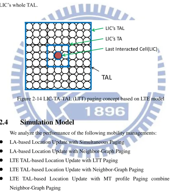
Thus, the paging scheme is executed when call arrival comes. The system will first page the UE’s Last Interacted Cell (LIC), which is the last cell where the UE has interaction with the network (i.e. be paged or performing LU). If the UE is not found in LIC, the system will page the whole LIC’ LA.

2.3.2 Neighbor Graph Paging

With the knowledge of Neighbor Graph which we have discussed in 2.1.1, each cell has its neighbor cells. When there is a call arrival coming, the paging process will be executed as following process. At first, the system will page the LIC. However, if the UE is not found in LIC, the system will page the LIC’s neighbor cells. If the UE still not found, the system will page the neighbor cells of LIC’s neighbor cells. Figure 2-10 shows the concept, paging one by one level from inner cell R0 until the system find the UE.

(32)

22

Figure 2-10 The Neighbor-Graph paging concept

If the Neighbor Graph paging is used on LTE configuration, the paging process is the same as first paragraph, but there is a paging upper bound which is the LIC’s TAL. Figure 2-11 illustrates the situation.

Figure 2-11 The Neighbor-Graph paging concept based on LTE model

2.3.3 Mobile Terminating (MT) Profile Paging

The MT profile paging scheme is based on the concept of Mobile Terminating matrix; we know the traffic model between cells. Thus, for the paging process is as following and shown in figure 2-12. First, the system page the last interacted cell (LIC). If the UE is found, the system finishes paging. If the UE is not found in LIC, the system would page the LIC’s MT profile, the most possible visited cells. If the UE still not found, the system would page the LIC’s TA, and search the UE. If the UE is not located in the TA, the system would page the LIC’s whole TAL.

(33)

23

Figure 2-12 MT profile paging concept based on LTE model

2.3.4 MT Profile Paging based on Neighbor Graph

According to the knowledge of traffic model between cells (Mobile Terminating matrix) and HO statistics (Neighbor Graph), we are able to combine the advantages of these two strategies. Based on the TAL model, figure 2-13 illustrates the concept. First, the system page the last interacted cell (LIC). If the UE is found, the system finishes paging. If the UE is not found in LIC, the system would page the LIC’s MT profile, the most possible visited cells. If the UE still not found, the system would page the LIC’s neighbor cells, and search the UE. If the system cannot reach the UE, the system will page the neighbor cells of LIC’s neighbor cells. And the process goes like this, paging one by one level from inner cell LIC until the system find the UE. It is important to mention that the paging upper bound is the LIC’s whole TAL.

(34)

24

LTE model

2.3.5 LIC-TA-TAL (LTT) Paging

Based on LTE model, the paging scheme [4] use the structure of TA and TAL. As figure 2-14 shows, when there is a call arrival coming, the system would first page the last interacted cell (LIC) to reach the UE. If the UE is not found, the system would page the LIC’s TA. If the system cannot reach the UE, the paging process will then page the LIC’s whole TAL.

Figure 2-14 LIC-TA-TAL (LTT) paging concept based on LTE model

2.4 Simulation Model

We analyze the performance of the following mobility managements:  LA-based Location Update with Simultaneous Paging

 LA-based Location Update with Neighbor-Graph Paging  LTE TAL-based Location Update with LTT Paging

 LTE TAL-based Location Update with Neighbor-Graph Paging

 LTE TAL-based Location Update with MT profile Paging combine with Neighbor-Graph Paging

We investigate the performance of the location update schemes and paging schemes which we described in previous sections. We consider four performance measurements:

(35)

25

 Npu : number of Periodic Location Updates (PLU) or Periodic Tracking Area Update (PTAU)

 Np : number of cells paged when incoming calls arrives

Because the whole system is an event-triggered algorithm, thus, we will explain events one by one in the following sections.

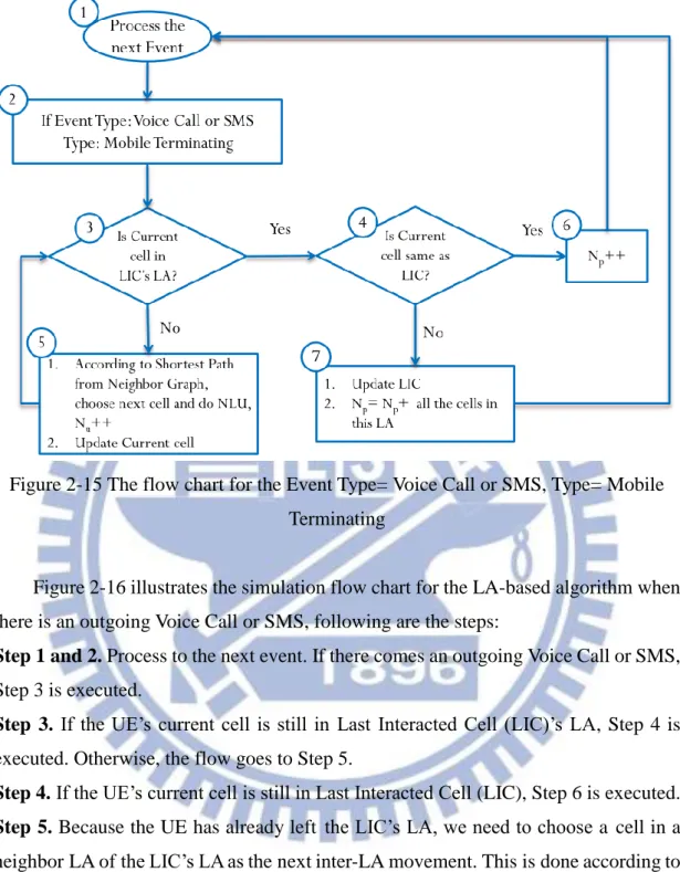
2.4.1 LA-based Location Update with Simultaneous Paging

The UE executes the location update procedure to inform the network of its new location whenever it enters a new LA. When an incoming call arrives, the network searches the UE by broadcasting the paging message to all cells in the last interacted cell (LIC)’s LA.

Figure 2-15 illustrates the simulation flow chart for the LA-based algorithm when there is an incoming Voice Call or SMS. Following are the steps:

Step 1 and 2. Process to the next event. If there is an incoming Voice Call or SMS, Step 3 is executed.

Step 3. If the UE’s current cell is still in Last Interacted Cell (LIC)’s LA, Step 4 is executed. Otherwise, the flow goes to Step 5.

Step 4. If the UE’s current cell is still in Last Interacted Cell (LIC), Step 6 is executed. Otherwise, the flow goes to Step 7.

Step 5. Because the UE has already left the LIC’s LA, we need to choose a cell in a neighbor LA of the LIC’s LA as the next inter-LA movement. This is done according to the shortest path found by the neighbor graph, and Nu is incremented by one. Then, update the LIC to the chosen cell and the flow goes to Step 3.

Step 6. The UE’s current cell still resides in the last interacted cell, so the Np was

incremented by one, and proceeds to Step 1.

Step 7. The UE’s current cell has moved out from the last interacted cell, the cellular network system sends the paging message to the cells in the last interacted cell’s LA. Then, the flow goes to Step 1.

(36)

26

Figure 2-15 The flow chart for the Event Type= Voice Call or SMS, Type= Mobile Terminating

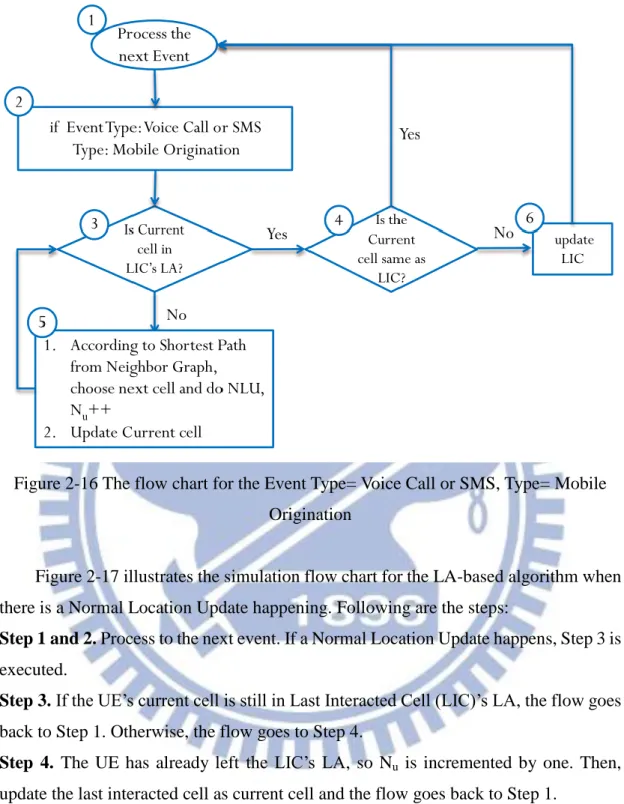
Figure 2-16 illustrates the simulation flow chart for the LA-based algorithm when there is an outgoing Voice Call or SMS, following are the steps:

Step 1 and 2. Process to the next event. If there comes an outgoing Voice Call or SMS, Step 3 is executed.

Step 4. If the UE’s current cell is still in Last Interacted Cell (LIC), Step 6 is executed. Step 5. Because the UE has already left the LIC’s LA, we need to choose a cell in a neighbor LA of the LIC’s LA as the next inter-LA movement. This is done according to the shortest path found by the neighbor graph, and Nu is incremented by one. Then, update the LIC to the chosen cell and the flow goes to Step 3.

(37)

27

Figure 2-16 The flow chart for the Event Type= Voice Call or SMS, Type= Mobile Origination

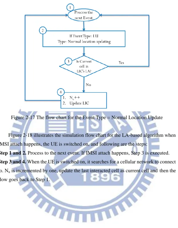
Figure 2-17 illustrates the simulation flow chart for the LA-based algorithm when there is a Normal Location Update happening. Following are the steps:

Step 1 and 2. Process to the next event. If a Normal Location Update happens, Step 3 is executed.

Step 3. If the UE’s current cell is still in Last Interacted Cell (LIC)’s LA, the flow goes back to Step 1. Otherwise, the flow goes to Step 4.

Step 4. The UE has already left the LIC’s LA, so Nu is incremented by one. Then,

(38)

28

Figure 2-17 The flow chart for the Event Type = Normal Location Update

Figure 2-18 illustrates the simulation flow chart for the LA-based algorithm when IMSI attach happens, the UE is switched on, and following are the steps:

Step 1 and 2. Process to the next event. If IMSI attach happens, Step 3 is executed. Step 3 and 4. When the UE is switched on, it searches for a cellular network to connect to. Nu is incremented by one, update the last interacted cell as current cell and then the flow goes back to Step 1.

(39)

29

Figure 2-18 The flow chart for the Event Type = IMSI attach

Figure 2-19 illustrates the simulation flow chart for the LA-based algorithm there is a Periodic Location Update happen, the UE is switched on, and following are the steps:

Step 1 and 2. Process to the next event. There is a Periodic Location Update happen, the UE regularly report its location at a set time interval. Step 3 is executed.

Step 3 and 4. Npu is incremented by one, update the last interacted cell as current cell

(40)

30

Figure 2-19 The flow chart for the Event Type = Periodic Location Update

2.4.2 LA-based Location Update with Neighbor-Graph

Paging

The UE executes the location update procedure to inform the network of its new location whenever it enters or leaves the LA boundary. When an incoming call arrives, the network searches the UE by first page the last interacted cell (LIC), then LIC’s neighbor cells, and then the neighbor cells of LIC’s neighbor cells, paging one by one level from inner cell LIC to outer neighbor cells until the system find the UE.

Figure 2-20 illustrates the simulation flow chart for the Neighbor Graph-based algorithm when there is an incoming Voice Call or SMS, following are the steps: Step 1 and 2. Process to the next event. If there is an incoming Voice Call or SMS, Step 3 is executed.

Step 4. If the UE’s current cell is still in Last Interacted Cell (LIC), Step 6 is executed. Otherwise, the flow goes to Step 7.

(41)

31

neighbor LA of the LIC’s LA as the next inter-LA movement. This is done according to the shortest path found by the neighbor graph, and Nu is incremented by one. Then, update the LIC to the chosen cell and the flow goes to Step 3.

Step 7. The UE’s current cell has moved out last interacted cell, the cellular network system sends the paging message to the cells which are LIC’s neighbor in the layer of next Distance. Then, the flow goes to Step 8.

Step 8. If the current cell resides in the neighbors where just paged in Step 7, Step 9 is executed. Otherwise, the flow goes to Step 7.

Step 9. The current cell is found in the neighbors, Np is incremented by one plus all the

cells inside the layer of Distance. Then, update the last interacted cell with current cell and the flow goes to Step 1.

Figure 2-20 The flow chart for the Event Type= Voice Call or SMS, Type= Mobile Terminating

Figure 2-21 illustrates the simulation flow chart for the Neighbor Graph-based algorithm when there is an outgoing Voice Call or SMS happens, following are the steps:

(42)

32

Step 1 and 2. Process to the next event. If there comes an outgoing Voice Call or SMS happens, Step 3 is executed.

Step 4. If the UE’s current cell is still in Last Interacted Cell (LIC), the flow goes back to Step 1. Otherwise, the flow goes to Step 6.

Step 5. Because the UE has already left the LIC’s LA, we need to choose a cell in a neighbor LA of the LIC’s LA as the next inter-LA movement. This is done according to the shortest path found by the neighbor graph, and Nu is incremented by one. Then, update the LIC to the chosen cell and the flow goes to Step 3.

Step 6. The system update UE’s last interacted cell with current cell and proceeds to Step 1.

Figure 2-21 The flow chart for the Event Type = Voice Call or SMS, Type = Mobile Origination

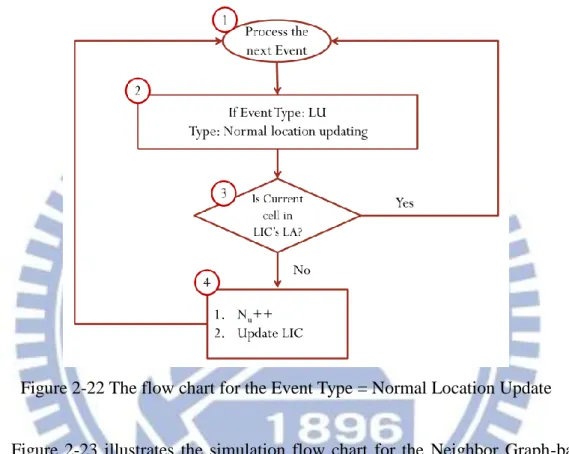
Figure 2-22 illustrates the simulation flow chart for the Neighbor Graph-based algorithm when there is a Normal Location Update happening, following are the steps: Step 1 and 2. Process to the next event. If a Normal Location Update happens, Step 3 is

(43)

33

executed.

Step 3. If the UE’s current cell is still in Last Interacted Cell (LIC)’s LA, the flow goes back to Step 1. Otherwise, the flow goes to Step 4.

Step 4. The UE has already lefts the LIC’s LA, so Nu is incremented by one. Then,

update the last interacted cell as current cell and the flow goes back to Step 1.

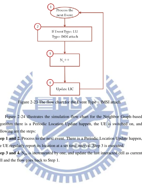
Figure 2-23 illustrates the simulation flow chart for the Neighbor Graph-based algorithm when IMSI attach happen, the UE is switched on, and following are the steps: Step 1 and 2. Process to the next event. If IMSI attach happens, Step 3 is executed. Step 3 and 4. When the UE is switched on, it searches for a cellular network to connect to. Nu is incremented by one, and update the last interacted cell as current cell and the flow goes back to Step 1.

(44)

34

Figure 2-24 illustrates the simulation flow chart for the Neighbor Graph-based algorithm there is a Periodic Location Update happen, the UE is switched on, and following are the steps:

Step 3 and 4. Npu is incremented by one, and update the last interacted cell as current

(45)

35

2.4.3 LTE TAL-based Location Update with LIC-TA-TAL

(LTT) Paging

The UE executes the location update procedure to inform the network of its new location whenever it enters or leaves TAL. When an incoming call arrives, the network searches the UE by first paging the last interacted cell (LIC), then LIC’s TA, and then LIC’s TAL.

Figure 2-25 illustrates the simulation flow chart for the LTE TA & TAL algorithm when there is an incoming Voice Call or SMS, following are the steps:

Step 3. If the UE has been idle over the set time, Step 4 is executed. Otherwise, the flow goes to Step 5.

Step 4. The UE need to do a periodic location update, Npu is incremented by one, and

process to Step 5.

Step 5. If the UE is still resides the Tracking Area List (TAL), Step 6 is executed. Otherwise, the flow goes to Step 7.

(46)

36

Otherwise, the flow goes to Step 9.

Step 7. Because the UE has already left the LIC’s TAL, we need to choose a cell in a neighbor TA of the LIC’s TAL as the next inter-TAL movement. This is done according to the shortest path found by the neighbor graph, and Nu is incremented by one. Then, update the TA and TAL according to the chosen cell and the flow goes to Step 5.

Step 8. The UE’s current cell still resides in the last interacted cell. So the Np was

Step 9 and 10 and 11. If the UE’s current cell resides in the TA, the Np is incremented

by the number of cells inside TA, and update the TA and TAL by current cell. Flow goes back to Step1. Otherwise, the UE’s current cell has moved out last interacted cell’s TA, resides in TAL, the cellular network system sends the paging message to the cells in the last interacted cell’s TAL. Np is incremented by the number of cells in TAL, and update the TA and TAL by current cell, and the flow goes to Step 1.

Figure 2-25 The flow chart for the Event Type = Voice Call or SMS, Type = Mobile Terminating

(47)

37

Figure 2-26 illustrates the simulation flow chart for the LTE TA & TAL algorithm when there is an outgoing Voice Call or SMS happens, following are the steps:

process to Step 5.

Step 6. If the UE’s current cell is still in Last Interacted Cell (LIC)’s TA, the flow goes back to Step 1. Otherwise, the flow goes to Step 8.

Step 8. The UE is reside inside TAL, but not in TA. Update TA and TAL with current cell, and flow goes back to Step 1.

(48)

38

Figure 2-27 illustrates the simulation flow chart for the LTE TA & TAL algorithm when there is a Normal Location Update happen, following are the steps:

process to Step 5.

Step 5. If the UE is still resides the Tracking Area List (TAL), the flow goes back to Step 1.Otherwise, the flow goes to Step 6.

Step 6. Because the UE has already left the LIC’s TAL, we need to choose a cell in a neighbor TA of the LIC’s TAL as the next inter-TAL movement. This is done according to the shortest path found by the neighbor graph, and Nu is incremented by one. Then, update the TA and TAL according to the chosen cell and the flow goes to

(49)

39

Step 5.

Figure 2-28 illustrates the simulation flow chart for the LTE TA & TAL algorithm when IMSI attach happen, the UE is switched on, and following are the steps:

Step 1 and 2. Process to the next event. If IMSI attach happens, Step 3 is executed. Step 3 and 4. When the UE is switched on, it searches for a cellular network to connect to. Nu is incremented by one, update the TA and then TAL with current cell and the flow goes back to Step 1.

(50)

40

Figure 2-29 illustrates the simulation flow chart for the LTE TA=eNB & TAL algorithm there is a Periodic Location Update happening, the UE is switched on, and following are the steps:

Step 1 and 2. Process to the next event. There is a Periodic Location Update happening, the UE regularly report its location at a set time interval. Step 3 is executed.

Step 3. If the UE has been idle over the set time, Step 4 is executed. Otherwise, the flow goes back to Step 1.

Step 4. Npu is incremented by one, update TA and TAL with current cell and then the

(51)

41

2.4.4 LTE TAL-based Location Update with

Neighbor-Graph Paging

The UE executes the location update procedure to inform the network of its new location whenever it enters or leaves TAL. When an incoming call arrives, as figure 2-11 shows, the network searches the UE by first page the last interacted cell (LIC), then LIC’s neighbor cells, and then the neighbor cells of LIC’s neighbor cells, page one by one level from inner cell LIC to outer neighbor cells until the system find the UE. It is important to mention that the paging upper bound is the LIC’s whole TAL.

Figure 2-30 illustrates the simulation flow chart for the LTE TA & TAL with Neighbor Graph-based paging algorithm when there is an incoming Voice Call or SMS, following are the steps:

(52)

42

process to Step 5.

Step 6. If the UE’s current cell is still in Last Interacted Cell (LIC). Step 8 is executed. Otherwise, the flow goes to Step 9.

Step 9. The UE’s current cell has moved out last interacted cell, the cellular network system sends the paging message to the cells which are LIC’s neighbor in the layer of next Distance. Then, the flow goes to Step 10.

Step 10 and 11. Check if the current paging area has over the TAL size, if it is true, Nu

is incremented by one, and update the TA and TAL with current cell. Flow goes back to Step 1. Otherwise, flow proceeds to Step 12.

Step 12. If the current cell resides in the neighbors where just paged in Step 9, Step 13 is executed. Otherwise, the flow goes back to Step 9.

Step 13. The current cell is found in the neighbors, Np is incremented by all the cells

inside the layer of Distance. Then, update the TA and TAL with current cell and the flow goes to Step 1.

(53)

43

Figure 2-30 The flow chart for the Event Type = Voice Call or SMS, Type = Mobile Terminating

Figure 2-31 illustrates the simulation flow chart for the LTE TA & TAL with Neighbor Graph-based paging algorithm when there is an outgoing Voice Call or SMS happens, following are the steps:

process to Step 5.

Step 6. If the UE’s current cell is still in Last Interacted Cell (LIC)’s TA, the flow goes back to Step 1. Otherwise, the flow goes to Step 8.

Step 7. Because the UE has already left the LIC’s TAL, we need to choose a cell in a neighbor TA of the LIC’s TAL as the next inter-TAL movement. This is done

(54)

44

according to the shortest path found by the neighbor graph, and Nu is incremented by one. Then, update the TA and TAL according to the chosen cell and the flow goes to Step 5.

Step 8. The UE resides inside TAL, but not in TA. Update TA and TAL with current cell, and flow goes back to Step 1.

Figure 2-32 illustrates the simulation flow chart for the LTE TA & TAL with Neighbor Graph-based paging algorithm when there is a Normal Location Update happen, following are the steps:

(55)

45

process to Step 5.

Step 5. If the UE is still resides the Tracking Area List (TAL), the flow goes back to Step 1.Otherwise, the flow goes to Step 6.

Step 6. Because the UE has already left the LIC’s TAL, we need to choose the cell as next movement according to the shortest path learned by neighbor graph, and Nu is incremented by one. Then, update TA and TAL with the cell just chosen and the flow goes back to Step 5.

Figure 2-33 illustrates the simulation flow chart for the LTE TA & TAL with Neighbor Graph-based paging algorithm when IMSI attach happen, the UE is switched on, and following are the steps:

Step 1 and 2. Process to the next event. If IMSI attach happens, Step 3 is executed. Step 3 and 4. When the UE is switched on, it searches for a cellular network to connect to. Nu is incremented by one, update the TA and then TAL with current cell and the flow goes back to Step 1.

(56)

46

Figure 2-34 illustrates the simulation flow chart for the LTE TA & TAL with Neighbor Graph-based paging algorithm there is a Periodic Location Update happen, the UE is switched on, and following are the steps:

Step 3. If the UE has been idle over the set time, Step 4 is executed. Otherwise, the flow goes back to Step 1.

Step 4. Npu is incremented by one, and update TA and TAL with current cell and the

(57)

47

2.4.5 LTE TAL-based Location Update with MT Profile

Paging and Neighbor-Graph Paging

The UE executes the location update procedure to inform the network of its new location whenever it enters or leaves TAL. When an incoming call arrives, as figure 2-13 shows, the network searches the UE by first page the last interacted cell (LIC), then LIC’s mobile terminating (MT) profile which are the most possible visited cells, and then the LIC’s neighbor cells, following with the neighbor cells of LIC’s neighbor cells, page one by one level from inner cell LIC to outer neighbor cells until the system find the UE. It is important to mention that the paging upper bound is the LIC’s whole TAL.

Figure 2-35 illustrates the simulation flow chart for the LTE TA & TAL with Sequential paging and Neighbor Graph-based paging algorithm when there is an incoming Voice Call or SMS, following are the steps:

(58)

48

3 is executed.

process to Step 5.

Step 6. If the UE’s current cell is still in Last Interacted Cell (LIC). Step 8 is executed. Otherwise, the flow goes to Step 9.

Step 9. The UE’s current cell has moved out last interacted cell, the cellular network system sends the paging message to the LIC’s MT profile, which are the most probable cells that the LIC would visit. If the UE is found, Step 10 is executed. Otherwise, the flow goes to Step 11.

Step 10. The current cell is found in the MT profile, Np is incremented by all the cells

inside MT profile. Then, update the TA and TAL with current cell and the flow goes to Step 1.

Step 11. Check if the UE is found in the LIC’s neighbor cells. If it is true, Step 12 is executed. Otherwise, the flow goes to Step 13.

Step 12. The UE is found in the neighbor cells, Np is incremented by all the cells inside

the neighbors. Then, update the TA and TAL with current cell and the flow goes to Step 1.

Step 13. The UE is not found in neighbor cells, thus, the paging process to the next level of neighbor cells. Then the flow goes to Step 14

Step 14. Check if the current paging area has over the TAL size, if it is true, the flow goes to Step 15. Otherwise, flow proceeds to Step 11.

行動通訊網路之移動管理分析

國

立

交

通

大

學

資訊科學與工程研究所

碩

士

論

文

行動通訊網路之移動管理分析

An Analysis of Mobility Management for Cellular Networks

研 究 生：蘇郁晴

指導教授：張明峰 教授

行動通訊網路之移動管理分析

An Analysis of Mobility Management for Cellular Networks

研 究 生：蘇郁晴 Student：Yu-Chin Su

指導教授：張明峰 Advisor：Ming-Feng Chang

國 立 交 通 大 學

資 訊 科 學 與 工 程 研 究 所

碩 士 論 文

行動通訊網路之移動管理分析

學生 : 蘇郁晴 指導教授 : 張明峰

國立交通大學資訊工程研究所 碩士班

摘要

An Analysis of Mobility Management for Cellular Networks

Student: Yu-Chin Su Advisor: Prof. Ming-Feng Chang

Institute of Computer Science and Engineering

National Chiao Tung University

Abstract

誌謝

Contents

List of Figures

List of Tables

Chapter 1 Introduction

1.1

Overview

1.2

Motivation

1.3

Traditional Mobility Management

1.3.1 Location Update Schemes

1.3.2 Paging

1.4

Long Term Evolution (LTE)

1.5

The History Signaling Records.

1.6

Objective

1.7

Summary

Chapter 2 System Configuration and

Implementation

2.1

Service Area Configuration

2.1.1 Neighbor Graph

2.1.2 Mobile Terminating (MT) Matrix

2.1.3 LTE Tracking Area List Model

2.2

Tracking Area Planning

2.2.1 Partition based on Handoff (HO) Rates

2.2.2 Mobile Termination (MT) Graph Partition

2.2.3 Real Distance Partition

2.3

Paging Scheme

2.3.1 Simultaneous Paging

2.3.2 Neighbor Graph Paging

2.3.3 Mobile Terminating (MT) Profile Paging

2.3.4 MT Profile Paging based on Neighbor Graph

2.3.5 LIC-TA-TAL (LTT) Paging

2.4

Simulation Model

2.4.1 LA-based Location Update with Simultaneous Paging

2.4.2 LA-based Location Update with Neighbor-Graph

Paging

2.4.3 LTE TAL-based Location Update with LIC-TA-TAL

(LTT) Paging

2.4.4 LTE TAL-based Location Update with

研究生：蘇郁晴

指導教授：張明峰教授

研究生：蘇郁晴 Student：Yu-Chin Su

國立交通大學

資訊科學與工程研究所

碩士論文

學生 : 蘇郁晴指導教授 : 張明峰

國立交通大學資訊工程研究所碩士班