國
立
交
通
大
學
統 計 學 研 究 所
博 士 論 文
利用統計方法自動依工程忍受度判斷機台差異
及其在半導體製程改善之應用
A New Statistical Method for Automatic
Partitioning Tools According to Engineers’
Tolerance Control in Process Improvement
研 究 生:涂凱文
指導教授:盧鴻興 教授
利用統計方法自動依工程忍受度判斷機台差異及其
在半導體製程改善之應用
A New Statistical Method for Automatic Partitioning
Tools According to Engineers’ Tolerance Control in
Process Improvement
研 究 生:涂凱文 Student:Kai-Wen Tu
指導教授:盧鴻興 Advisor:Dr. Henry Horng-Shing Lu
國 立 交 通 大 學
統 計 學 研 究 所
博 士 論 文
A Thesis
Submitted to Institute of Statistics College of Science National Chiao Tung University
in partial Fulfillment of the Requirements for the Degree of Ph. D
in
Institute of Statistics August 2008
Hsinchu, Taiwan, Republic of China
A New Statistical Method for Automatic Partitioning Tools
According to Engineers’ Tolerance Control in Process Improvement
Student:Kai-Wen Tu Advisor:Dr. Henry Horng-Shing Lu
Institute of Statistics
National Chiao Tung University
ABSTRACT
In the semiconductor industry, tool comparison is a key task in the yield and the product quality enhancements. We developed a new method, called tolerance control partitioning (TCP), to automatically partition tools into several homogenous groups based on the related metrology results. This methodology is based on a hierarchical normal model and the implementation is carried out using a Bayesian approach. There are several advantages of using the TCP method. First, it takes into account the unbalanced usage of the tools in the manufacturing processes. Moreover, the “engineer’s tolerance control” can be incorporated into the TCP method via the specification of the priors in the Bayesian analysis, which justifies the significant difference between groups according to the experts’ knowledge. This specification not only has the advantage of adjusting the number of partition groups but also avoids the problem of having too many partition groups with small differences which is often encountered in the conventional approaches. Some simulation results illustrate the advantages of the TCP method compared to the method of classification
and regression trees (CART). Moreover, the TCP method is applied to two real examples for the yield and Cp/Cpk enhancement in the semiconductor industry. Both results confirm the practical usefulness of the proposed method. For general applications, the TCP method is also useful for other similar problems such as the comparisons between several experimental recipes or the comparisons between different materials.
Acknowledgements
謹寫下這段致謝文感謝所有人,也作為自己人生的反省與珍貴的回憶。 決定重回已經離開十多年的學生生涯,其實不只是想再充實自己統計的專 長,也是完成自己年少的夢想。只是時光飛逝一去不回,當時年少的我,如今 已是身兼公司員工,兩個小孩的爸爸等多重身份的中年男子。 早上上班,晚上唸書的日子,讓日子每天都過得很快,常常累到想像自己 是一位精疲力竭的劍客,用劍撐著疲痛的身軀,但卻又得目光銳利地看著下一 個目標,準備前去。身體是疲憊的但卻鬥志高昂。如今博士生涯將近尾聲,其 中的感觸非筆墨所能形容。我想千言萬語還是感謝兩字。 要感謝的人太多了! 感謝清華統計所的趙蓮菊老師,專業又高水準的統計推論課程,讓我快速 進入〝博士生〞的狀況。更感謝她體諒我因家人患病那段日子分心無法兼顧學 業,要不是她的一念之仁,我想我的博士生涯可能會有完全不同的結果。 感謝我碩士班指導教授陳鄰安老師,從我準備入學到畢業,總是給我很多 鼓勵和幫助,並時常分享一些做學問的心得和指引我一些未來的方向,讓我受 用不盡。我相信老師會是我一輩子的好朋友。 感謝陳志榮老師提供的高等機率論課程,他的教導方式,讓我對一直最害 怕的科目,找到全新的學習方式,這對我通過資格考幫助很大。 感謝我的良師益友清華統計所的徐南蓉老師,雖然是大學同學,但卻是我 博士生涯的學習導師,總是在我學習遇到困境時成為最佳的諮詢對象,也省下 很多徒勞蹉跎的時光。在課堂上聽她精采的時間序列課程也是博士生涯中一大 享受。感謝也懷念我已故的恩師李昭勝老師,我從他身上學到了如何對後生晚輩 提攜,鼓勵和支持。在我的博士路上,每當遇到困難,他總是提供了最有效的 幫忙,他的鼓勵常常讓心情低落的我注入強心劑。心情安頓好了,就有再衝刺 的力量。我想他給了我很多的信心,有時我甚至感覺老師比我對自己還有信心。 而這是對一位離開十多年學生生涯的在職生最需要的。我更感謝他對我在博士 學習規劃上的尊重。讓我有更多的發揮空間。而他對學術的熱忱,也是身為後 生晚輩的我最佳的典範。我想我這〝問題〞學生可能讓他多操勞了!他的離開 讓我有無限的感傷與懷念。「哲人日已遠,典型再夙昔」,他對我的師恩,將永 生難忘。他對我的提點,會是我不斷努力下去的動力。 感謝我的指導教授盧鴻興老師,感謝他願意伸出援手,協助我,指導我完 成博士求學的最後一段路,老師對學術的熱忱也是值得我再三學習的。 感謝所上的秘書郭姐,對我這個常常不在所上的特殊學生,提供特別的服 務,讓我這〝忙碌的〞在職生方便許多,我在博士路上最後的小插曲也必須感 謝她盡力的幫忙,很抱歉造成她的困擾。 也感謝所上其他授課老師的指導。 感謝交大統計所,開了一扇門,讓一位〝工業界〞的在職生有機會再接觸、 再學習統計,我相信這將會鼓勵更多充滿熱情的統計工作者,再成長的機會。 也會成為在業界打拼的統計人最佳的後盾。 感謝我公司的長官潘文森副總、古延輝協理與彭誠湧資深處長的支持,他 們用行動表現出工業界對統計的重視,並提供了統計工作者再進步,再成長的 機會。同時也感謝我公司的工作夥伴們,因為他們的優異表現,讓我在博士求 學過程無後顧之憂。我也必須感謝在公司的一些好朋友們時常關心我的近況, 雖然只是兩句關心的話語卻讓我再度充滿信心。 感謝我的口試委員洪志真老師、曾勝滄老師、黃榮臣老師及黃信誠老師,
對我的建議和指導,讓我對論文撰寫與學術嚴謹的態度永生難忘。也讓我對教 育有新一層的體會。想起已故李昭勝老師常提醒我的一句話 “ Good Luck is always with well preparation" 我想一切還是因為自己做的不夠好,我會繼 續努力。
感 謝 國 際 期 刊 IEEE Transactions on Semiconductor Manufacturing 的 editor 及 reviewer 協助審核並 Accept 我的博士論文。可以發表文章在國際期 刊一直是我在博士學習過程設定最大的目標。很高興我做到了,它真的給了我 很大的信心與鼓勵。從自己在業界找題目、學統計技術、腸枯思竭想方法、挑 燈夜戰做 simulation、做出成果、學習寫論文、學習打字到發表。心理上經歷了 被國際期刊拒絕的失望感及苦苦等待國際期刊回覆的苦悶感到最後被國際期刊 接受那不可思議的驚喜。很高興我在博士生的階段走完全程。這些點點滴滴將 會是我人生中一段重要的回憶也是我下階段再出發最有幫助的經驗。 最後,我必須送上我最深的感謝給我的家人,畢竟身為人父、人夫、人 子,做任何決定都將影響一家人的生活。感謝我的父、母、岳父、岳母對我的 支持。我拿到博士學位,他們甚至比我還高興。感謝我兩位可愛的兒子光遠、 光庭,他們不但乖巧懂事讓我不用分心,還會偶而做卡片鼓勵爸爸〝要保重, 要加油〞。爸爸的博士之旅相信也讓他們感受到爸爸對讀書的熱情,希望這對他 們的求學過程會有幫助。感謝我的賢內助李柏青小姐,雖然她工作家庭兩頭忙 十分辛苦,但卻願意成就一位愛唸書老公的夢想。因為我的博士路讓她少了很 多戶外郊遊、逛街及休息的機會也少了很多老公的寒喧問暖。我會十分珍惜人 生路上老婆給我這圓夢的機會,我應該也為她戴上博士的方帽,以感謝她為我 與家庭的犧牲與付出。〝老婆謝謝您〞。
Contents
Abstract ………..i
Acknowledgements………...iii
1. Introduction ………..…… 1
2. Methodologies ……….…...9
2.1 A Hierarchical Bayesian Model for Partition Problems……….9
2.2 Reversible Jump Markov Chain Monte Carlo………...…12
2.3 TCP Method for Tool Partitions ……… 15
2.4 Guidelines for Choosing Initial Values for Parameters and Hyperparameters in TCP………...19
2.5 Convergence Assessment for RJMCMC………...…………...21
3. Simulation Studies ...24
3.1 Unbalanced data for unbalance tool usages………...…………25
3.2 Sensitivity Analysis with Different Tolerance Controls for TCP and the Comparison with CART……….…..34
3.3 Robustness Studies by Balanced Simulation Data with Mean Shifts…..….38
4. Two Applications in the Semiconductor Industry. ………43
4.1 Ramp Up Yield Using the TCP Method……….….43
4.2 Process Capability Indices Enhancement………...49
5. Conclusion and Discussion………...58
6. Future Works ………61
7. Appendix ………...63
1. Introduction
The importance of semiconductor technology in today’s world can hardly be
exaggerated. Semiconductor devices are absolutely essential components for almost
all electronic products. Without semiconductors, most of the electronic products and
the systems cannot be made or operated and their influences on human society are
beyond belief. The global semiconductor industry had around US$230 billion worth
of revenue in 2005 and keeps creating new opportunities, socio-economic
advancements and new human developments to nations and societies around the
world [1]. Since building a modern wafer fabrication facility needs around US$3
billion, enhancing the yield rapidly to volume the production becomes an extremely
important source of the competitive advantage in the hyper-competitive world on
semiconductor manufacturing. The sooner a potentially lucrative circuit yields, the
better the manufacturer generates a revenue stream. On the other hand, rapidly
identifying the cause of yield loss can restore a revenue stream and prevent the
destruction of the materials in process [2] [3].
In the following, the semiconductor manufacturing is briefly introduced. It
follows a very complex process flow which is quite different from the traditional
making bare silicon wafers into integrated circuits, such as the microprocessors or the
memory chips. In general, 25 wafers are processed together in a group called a lot,
and the size of each wafer ranges from 3 to 12 inches in diameter. Each wafer could
contain thousands of dies depending on the size of the die being produced. During the
manufacturing process, the lots are manufactured through lots of process steps (more
than 150 process steps). Each process step involves several tools for production. After
completing each process step, the metrology systems collect the physical data and the
electrical data, such as the film thickness, film uniformity, critical dimension, overlay,
defect particle count, voltage, current and wafer sort, etc. At the end of the all process
steps, the Wafer Acceptance Test (WAT) with 100–500 electrical test items and the
Wafer Sort Test (WST) with 50-100 test items are performed sequentially to each
wafer. The objectives of WAT and WST are to perform the device characteristic
analysis and the die functionality sorting, respectively. Since these testing data also
characterize the quality of the manufacturing and the performance of the products,
therefore how to use these data to improve the process itself becomes an interesting
issue. However these data are huge with lots of variables (about 100M–1G for each
lot), it is very time-consuming for engineers to analyze the data and find out the
sources of variations in the production processes. Among various analyses, tool
effective and time-efficient method for comparing tools is critical for rapidly
improving the yields [4]. In the following, we briefly review the conventional
approaches in this area, including the multiple comparison methods and the clustering
methods.
For multiple comparisons, the analysis of variance (ANOVA) for normal data
and the Kruskal-Wallis test [5] for non-normal data are the two most popular
statistical methods for testing the significant differences between population means
among groups. For our tool partition problem, in order to compare the performances
among different tools (i.e., groups) at each process step, the engineers perform these
two statistical tests regarding the distribution of the considered metrology data
associated with each tool. By quickly reviewing the testing result for each individual
step, tool differences might be detected at certain process steps and an alarm will be
triggered for further checking or investigation. In general, the main purpose of this
kind of testing procedures is to find the variation sources (i.e., which process steps)
and identify the possibility of abnormal tools. After finding the significant differences
among tools at certain steps, the engineers will partition all the relevant tools into
several homogenous groups and further identify the best groups or the problematic
groups of tools in order to enhance the product quality or to exclude the worst tools,
for engineers but cannot be handled by the ANOVA or the Kruskal-Wallis test
simultaneously. Some multiple pairwise comparison procedures, such as the methods
suggested by Fisher [9], Tukey [10], Keuls [11], Duncan [12], Scheffe [13], and
Dunnett [14] [15], provide useful information about the ranking or ordering structures
of the group means but these methods cannot directly partition different tools (or
treatments) into homogenous and non-overlapping groups. For example, there are
three tools to be partitioned and their sample means satisfy Y 1 ≤ Y 2 ≤ Y 3 .
Suppose that a multiple comparison procedure finds that the differences
1 2
|Y − Y | and | Y 2 − Y 3 | are not significant but the difference
1 3
| Y − Y |is significant. It is not clear how to partition these three tools into homogenous but non-overlapping groups since both (Y 1,Y 2) and (Y 2,Y 3)
i P
are reasonable homogenous groups.
Another popular approach for partitioning is using the cluster analysis. Scott and Knott [16] suggested a procedure which starts by dividing the k means into two groups and then performs a test to decide whether the partition is acceptable. This approach is equivalent to a hypothesis testing problem:
0 1 2 1 1 2 : ... v . s . : ' e q u a l f o r , ' e q u a l f o r . i j H H s s j P κ
θ
θ
θ
θ
θ
= = = ∈ ∈where {P1,P2} forms a partition of
{
1, 2 , ...,
κ
}
and and are two disjoint and nonempty sets with1
P P2
1 2, {1, 2 , ..., }
at some chosen level
α
, similar testing procedure is then applied to each individual , i=1,2. The procedure is continued sequentially until all tests are not rejected (i.e.,no further partition is necessary). Worsley [17] proposed a nonparametric version of
Scott and Knott’s method. Although this approach is intuitive and easy to implement,
the Type I error of the entire test is difficult to control due to sequential testing
procedures, in particular when the number of splitting gets larger. Moreover, the final
partition result may not be unique which highly depends on the initial partition.
i
P
To overcome the difficulty of controlling the Type I error (the probability of
erroneous grouping) for the sequential testing procedure, Calinski and Corsten [18]
proposed two cluster methods to partition these tools (or treatments) in a balanced
design by embedding the simultaneous testing procedures based on F test and
Studentized range test, respectively. Although this approach solved the problem of
controlling Type I error, it still has several other disadvantages, such as the partition
groups are too many with small differences when the number of observations for each
tool is large; the issue about unbalance data is not considered which generally loses
the power when the usages are quite different among tools.
Jolliffe [19] proposed an alternative method to perform the cluster analysis.
This approach used a particular dissimilarity measure which is defined by the P-value
larger P-value indicates that two groups are more similar and a smaller P-value
indicates that two groups are more distinguishable. One critical issue for this
hierarchical clustering approach is to determine the number of clusters which is
usually determined subjectively.
Data mining approaches [20] [21], such as the classification and regression
trees (CART) [22] and the neural networks [23], have also been used for the partition
problem. Recently, some commercial data analysis software (for example: Yield
Dynamics, BI IBM, Odyssey YMS, and dataPOWER) in engineering use these
approaches for the yield enhancements. However, these approaches involve
supervised algorithms which rely on more complex initial parameter setups and the
partition results are usually sensitive to these setups [22], and therefore it is somehow
difficult for engineers to use them in practice. In Appendix A, the CART algorithm is
briefly introduced which will be compared with the proposed method in the
simulation study.
To sum up, each above-mentioned method has its own advantages and
disadvantages compared to the other methods under different circumstances. But none
of them is capable of incorporating the experts’ specific opinions into the statistical
analysis. For example, for our tool partition problem, the engineers’ tolerance controls
some way in the analysis on determining the grouping structure. Another challenge
for our tool partition problem in the manufacturing processes is to account for unequal
tool usages. Unequal usages for different tools at each process step make the numbers
of processed lots for each tool varying which induces unbalance data issue for the
statistical tests. Montgomery [24] addressed that the statistical tests for multiple
comparison lose power for unbalance data. The goal of this thesis is to develop a
method for tool partition which incorporates the experts’ specific opinions on the
tolerance of tool differences and considers the unbalance data issue simultaneously.
We formulate the tool partition problem as a hierarchical model [25] in which
the metrology measurements from each tool follow a normal distribution with
tool-specific mean. It is reasonable to expect that the tool-specific means for “similar
tools” are related in some way, such as viewing these tool-specific means as
realizations from the same distribution. Under this setup, the engineers’ tolerance of
tool differences can be naturally incorporated into the variance structure of the model
imposed on the tool-specific means. For such hierarchical models, Bayesian analysis
is the most popular method for inference in the literature. We will use the Bayesian
analysis for searching the possible grouping structure for different tools in which the
reversible jump Markov chain Monte Carlo (RJMCMC) algorithm, proposed by
“tolerance control partitioning” (TCP) which partitions tools into several homogenous
groups subject to the engineer’s specific tolerance about the mean differences.
The remainder of this paper is structured as follows. In Chapter 2, the
hierarchical model is introduced and the guidelines for choosing the priors for the
parameters and hyper-parameters in the Bayesian analysis are also addressed. In
Chapter 3, three simulation experiments are designed to illustrate the advantages of
using the TCP method. For comparison, the partition results using the pruning scheme
for the CART method (which also incorporates the tolerance of tool differences into
account) are also considered in the simulations. In Chapter 4, two real examples in the
semiconductor industry are analyzed for illustration. One example is related to the
yield enhancement and the other example is about the Cp/Cpk enhancement. In
addition, we propose two new ideas to integrate TCP with a statistical dashboard [4]
for yield enhancement and automatic process control (APC) [27]-[29] for Cp/Cpk
enhancement, respectively. In Chapter 5, some conclusions and discussions for the
TCP method are given. In Chapter 6, possible extensions of applying the TCP method
2. Methodologies
In this chapter, we introduce the TCP methodology. In Section 2.1, we
formulate our tool partition problem by a hierarchical Bayesian model. In Section 2.2,
we briefly introduce the reversible jump Markov chain Monte Carlo (RJMCMC)
method. In Section 2.3, we apply the RJMCMC to determine the best partition and
estimate the model parameters under a Bayesian approach for the tool partition
problem. In Section 2.4, we suggest some guidelines for the initial setups for the
model parameters and the hyper-parameters in the RJMCMC algorithm for the TCP
method. In Section 2.5, we describe the standard method for monitoring the
convergence of the Markov chain in the Bayesian context.
2.1 A Hierarchical Bayesian Model for Partition Problems
For each observation, Y denotes the response variable (e.g., the yield), and x
denotes the categorical predictor with J possible categorical levels (e.g., tools). The
conditional distribution of Y given x is,
Y
|
x
=
j
~ Normal (θj, ) for the j-thtool, and 2 σ 1 2 ( ,θ θ ,...,θJ) ' =
θ is the unknown parameter vector. The TCP method
{θj: j=1, 2,..., }J into several homogenous groups) according to the values of the response variable.
Each partition for J tools can be represented as a collection
g={ , ,…, } with groups and each group is a subset of {1, 2,…, J},
satisfying {1, 2,…, J} and for
1 S S2 Sκ κ Sk = ∪ = k k S κ
1 Si∩Sj =φ i≠ . The number of groups for j
the partition g, , determines the degree of heterogeneity among different tools.
According to the partition structure (or the grouping structure), we further assume that the mean parameters
κ
j
θ ’s follow the same normal distribution with the
hyper-parameters µk and τ when these θj’s belong to the same group Sk. That is,
j
θ ~ Normal (µk,τ 2) if j∈Sk, j=1,2,…,J.
If the partition g is known in advance, all the parameters can be easily
estimated by using the maximum likelihood. But, the partition g is unknown and a
Bayesian method is used for estimation. In the following, the prior distributions for
the mean and variance parameters and the related hyper-parameters are specified: (1) the prior for µk: (π µk)~ Uniform (a, b), for k=1,2,…, κ, and {µk} are
mutually independent,
(2) the prior for τ2: π τ( 2) is a scaled inverse chi-squared with degrees of
freedom ν and the scale parameter in which the
tolerance is a tuning parameter defined by the engineers to stand for the
2
6 s ≡(tolerance / )2
acceptable difference between tools,
(3) the prior for σ2: π σ( 2) is distributed as a scaled inverse chi-squared with degrees of freedom ν1 and the scale parameter s12.
For the partition g, following the specification in Consonni and Veronese [30], the
prior distribution is defined as
1
( )
{# partitions whose degree } g of κ π κ − ∝
= , where κ is the degree of partition g.
Under the above prior setup, the posterior distribution for the parameters satisfies 2 2 ( ) 1 1 1 1 1 2 2 2 2 2 2 2 2 2 2 ( ) 2 2 2 1/2 2 1/2 1 ( , , , , | ) ( , , , , , ) ( | , ) ( | , , ) ( ) ( ) ( ) ( ) 1 1 (2 ) (2 ) {# of partition n j J J J ij j j k j Sk j j i j k j y I n J p g p g p p g g e e κ θ θ µ σ τ σ τ σ τ σ τ π π π σ π τ πσ πτ κ ∈ = = = = = ⎛ ⎞ − − − ⎜⎜ − ⎟⎟ ⎝ ⎠ − ∝ = ∑∑ ∑ ∑ ∑ ⎛ ⎞ ⎛ ⎞ ∝ ⎜ ⎟ ⎜ ⎟ ⎝ ⎠ ⎝ ⎠ × θ µ θ µ θ θ µ µ y y y
(
)
1(
)
2 2 2 2 1 1 1 1 ( ( , )) 1 ( /2) ( /2) ( /2 1) /(2 ) 1 2 2 ( /2 1) 1 1 1 I s whose degree } / 2 / 2 ( ) ( ) ( / 2) ( / 2) k a b k s s b a s e s e κ κ µ ν ν ν ν ν σ ν ν ν /( 2 ) κ ν σ ν τ ν ν ∈ = − + − − + − ⎧ ⎫ ⎛ ⎞ ⎨ ⎬ ⎜ ⎟ = ⎝ − ⎠ ⎩ ⎭ × Γ ΓΠ
τ (1) where y={yij: j=1, 2,..., ;J i=1, 2,...,nj}, µ = (µ µ1, 2, ...,µκ) ', , and 1 k k g κ = = U S 1 2 (θ θ, , ...,θ ) ' = Jθ . This posterior for the model parameters does not has a close
form but is proportional to the joint distribution of the observed variables and the unknown parameters. For this kind of problem with unknown grouping structures, the
RJMCMC method is often used for the Bayesian implementation which is described
in the next subsection.
2.2 Reversible Jump Markov Chain Monte Carlo
The RJMCMC algorithm was initially proposed for the Bayesian model
determination problems [26]. But since then, it has been applied to many other
problems such as the change point problems, the mixture problem, and the factorial
experiments [26][31][32]. In the semiconductor manufacturing context, Bergeret and
Gall [33] have applied this algorithm to detect the change point for the yield trend
under the situation that the failure occurs at a problematic process stage and there are
different yield performances before and after the failure time. Moreover, the
RJMCMC algorithm has also been used with the CART method which leads to the
Bayesian CART method [34]-[38].
We present the RJMCMC algorithm as introduced in Green [26]. Suppose that
the competing models can be enumerable and are represented by the set of models
. Under the model
1 2
{M ,M , ... =
M } M k and given the data , the model
parameter
y
k
θ has the posterior distribution
( k | , ) ( | k , ) ( | )
where p( y |
θ
k ,k) and p(θ
k | k ) are the sampling distribution of and the prior distribution of the parametery
k
θ given the model M k , respectively. The
RJMCMC methods are an extension of the Metropolis-Hastings algorithm [39] that
allows a Markov chain not only moves between different parameter values but also
between models with different dimensions. This algorithm is designed to be reversible
so as to maintain detailed balance of a irreducible and aperiodic chain that converges
to the correct target posterior distribution. Please refer the reference [26] for the
details of RJMCMC.
In the following, we only conceptually illustrate the jumping scheme between
different models in the RJMCMC algorithm.
1. Propose a jump from the current Model M k to the other model M k ' with
probabilityJ M( k → M k ') .
2. Sample v from a proposal density q(v |
θ
k ,k k, ') , where is anaugmented variable which plays the role of adjusting the unequal dimension
problem between two models
v
k
M and M k '.
3. Set (
θ
k ',v ') = gk k, '(θ
k, )v , where gk k, '( )⋅ is called a bijectionfunction between (
θ
k ,v) and (θ
k ',v ') which provides a one-to-onemapping between two sets of parameters (
θ
k ',v ') and (θ
k ,v) and twoparameters for two model M k and M k ' .
4. The RJMCMC moves from the current model M k with parameter θk to
another model M k ' with parameter θk' according to the acceptance
probability r=min{1, }A where
' ' ' ' , ' ' ( , ) ( | , ') ( ) ( ') ( ) ( ' | , ', ) . ( | , ) ( ) ( ) ( ) ( | , , ') ( , ) k k k k k k k k k k k k k k g v p k p p k J M M q v k k A p k p p k J M M q v k k v ∂ → = → ∂ y y θ θ θ θ θ θ θ θ
Each iteration in the RJMCMC algorithm includes the above 4 steps and
repeating such iterations constructs a Markov chain. Under some appropriate setting
for the jumping scheme, this Markov chain will converge and its stationary
distribution is identical to the target posterior distribution of the parameters for the
selection problem among the model collection . The posterior distribution and
posterior mode for each parameter can be estimated using the MCMC draws after the
convergence is achieved. In particular, the model with the highest posterior
distribution on is considered as the best model based on the Bayesian approach
[35] [36] [40].
M
M
For our tool partition problem, the set consists of all possible partition
models with various degrees
M
g κ =1, 2,..., J . The RJMCMC algorithm helps us to
determine the best partition among tools and simultaneously estimate the model
parameters under the hierarchical Bayesian model. Although we did not give the
detail formulations for the functions involved in the jumping scheme (such
as J M( k → M k ') , gk k, '( )⋅ and q( |⋅
θ
k ,k k, ') since they are usually problem-specific, the detail scheme for our tool partition problem will be described inSection 2.3.
Moreover, we suggest the usage of posterior distribution of possible partitions
to realize the partitioning structure of tools instead of the usage of hierarchical tree
structures
2.3 TCP Method for Tool Partitions
In Section 2.1, the posterior distribution of ( , , ,g θ µ σ τ2, 2) given the data has been derived up to a normalizing constant. The posterior distribution as well as
the posterior mean for each parameter are estimated using the RJMCMC method. We
are particularly interested in the posterior distribution for which gives the best
partition for tools. The details about how to apply RJMCMC to our tool partition
problem in Section 2.2 which includes five move types:
y
g
1. updating the parameter of the group mean θj, for j=1, 2…J , 2. updating the parameter of the group variance σ2,
3. updating the hyperparameters τ2 and µk, for k=1, 2…κ,
5. updating the partition g, with “death”, that is, combining two groups into one.
At each iteration in the chain, one of the above five moves is randomly selected regarding some pre-set probabilities p p p p p , where 1, 2, 3, 4, 5 p is for the j -th
move type,
j
4
p and p usually depend on the degree of current partition g (i.e., 5
κ
)and . Naturally, we set
5 1 1 j j p = =
∑
p5 = when 0 κ = and 1 p4 = when is the 0maximum allowed value.
κ
Given the partition g in each MCMC iteration, the parameter values are
updated according to the conditional distributions of all parameters in the set =
{
Θ
1
θ , θ2… θJ, σ2, µ1, µ2… µκ, and } via the Gibbs sampling [41] [42] (Appendix B). We will use the notation of
2
τ
j
θ
−
Θ to indicate the set of all parameters
except the parameter of θj. The full conditional distributions of all parameters of are given below and the detailed derivations for these conditional distributions can be
found in Appendix C. Θ 1. θj| j θ − Θ ~ Normal ( j j a b 2 ,2aj 1 ), (2) where . 2 2 ( k j j) j n y b µ τ σ = + , 2 1 2 2 j j n a 2 τ σ = + , for j∈Sk, and j=1,2 ,…,J, 2. µk| k µ − Θ ~ Normal ( k j j S k w θ ∈∑ , 2 k w τ ) (a,b) k µ Ι where wk ={# of in }j Sk , 3. τ2 |Θ−τ2 ~ Inverse Gamma ( 2 J + ν , 2 2 s F ν + ), where F= , , 2 ( ) 1 1 k J j k j S j k I κ θ µ ∈ = = ⎛ − ⎞ ∑⎜ ∑ ⎟ ⎝ ⎠ k 1 k g κ S = = U
4. σ2|Θ−σ2 ~Inverse Gamma ( 2 1+N ν , 2 1 1 2 s E ν + ), where E= 2, and N= . 1 1 ) ( j n i ij J j j y θ ∑ − ∑ = = ∑= J j j n 1
The structure parameter g is updated by the birth and death move types. The
birth move means adding one group from the current partition g. In contrast, the death
move means eliminating one group from the current partition g. We introduce the
schemes for implementing these two move types below. Suppose that the current
partition is g(1) with degree
κ
(1) and mean vectorµ(1). For the “birth” move type, we first choose a group to split randomly among those with at least two tools to forma new partition g(2) with degree
κ
(2)= (κ
(1)+1) groups. At the same time, themean vector µ(2) needs a change for both the dimension and the value. The
relocation can be simply done by adding a new random variable z that is
independently distributed as Normal (µ ,z σ ). In Section 2.4, we will discuss how to 2z
define µ and z σ in detail. Suppose that a proposal birth splits group 2z for k
{1, 2… } into two groups and . Let
k S ∈ κ(1) 1 k S 2 k
S µk be the current value and
1 k µ ,
2 k
µ be the new values for the two groups. Then we set
1 k µ = µk + 2 2 k k w w z , 2 k µ = µk - 2 1 k k w w z , (3)
where ={# of j in } for i= , , and , with = + ,
= , and = i w Si k k1 k2 wk 1 k w 2 k w 1 k S ∪ 2 k S Sk 1 k S ∩ 2 k S φ. So we have g(2)={ (1) k s S − }∪{ , } and 1 k S 2 k S
1 2 ( 2) (1) ( , , k k k µ µ µ ) − =
µ µ . Similarly, for a “death” move, we will randomly choose two
groups and from the current partition and merge them into a new
group to generate a new partition with
1 k S 2 k S g(2) k S g(1) µk k1 k1 k2 k2 k w w w µ + µ = ,
= + , and by solving the simultaneous equations in (3).
k w 1 k w 2 k w 1 2 ( k k ) z= µ −µ wk
After specifying the jumping proposal, the acceptance probabilities for the
birth and death in the RJMCMC algorithm are min {1,A} and min{1,1/A} respectively,
where A = ( ) ( ) ( 2 ) 2 2 ( 2 ) (1) ( 2 ) ( 2 ) (1) 2 1 1 1 1 (1) (1) 1 (2) 2 1 (1) 1 I ( , ) ( ) 1 ( ) ( ) I ( , ) J J j k j k j S j S j k k j k k k k I I k d birth k a b P P g e b a P P g a b κ κ κ θ µ θ µ µ τ κ µ ∈ ∈ = = = = ⎧ ⎛ ⎞ ⎛ ⎞ ⎫ − ⎪∑ −∑ −∑ −∑ ⎪ ⎨ ⎜ ⎟ ⎜ ⎟ ⎬ ⎝ ⎠ ⎝ ⎠ ⎪ ⎪ = ⎩ ⎭ = Π × × − Π eath × # of {k;wk ≥2, k=1,2,…,κ }×(1) ) ( 1 1 } 2 2 { ) 1 ( 1 ) 1 ( ) 1 ( f z wk wk − + κ κ ,
where κ is the degree of (i) g(i), for i=1,2, with κ(2) =κ(1) +1, ,
is the number of tools in , are the proposal probability
for the death move type and birth move type respectively (i.e.,
( ) ( ) ( ) 1 i i i k k g κ S = = U k
w Sk(1) Pdeath, and Pbirth
4 p and p in the 5 earlier context), k w 1
is the Jacobian, and f(z) is the density function of z.
The derivations for the acceptance probabilities of the birth and death move types are
2.4 Guidelines for Choosing Initial Values for Parameters
and Hyperparameters in TCP
The engineers can set up the initial parameters and hyperparameters in the
priors based on their knowledge for each problem. However, when there is no
enough prior information, we will suggest some guidelines to set up the priors to
facilitate the practice of TCP in the semiconductor industry and in other applications.
The details of our guidelines include the following:
1. µk~ Uniform (a, b), for k=1,2,…,
κ
, let a=min {y.j: j=1,2,…,J} andb=max{y.j, j=1,2,…,J }. The reason is described as follows: Since these
j
θ ’s belong to the same group Sk, these θjs will be distributed as the same
normal distribution , (that is, θj ~ Normal ( µk , τ 2 ), for j ∈Sk ,
j=1,2,…,J . ) On the contrary, if 1 j θ and 2 j
θ belong to two different
groups and , 1 k S 2 k S 1 j θ and 2 j
θ are distributed as two different normal distribution with two different means
1 k µ and 2 k µ . Therefore, in tool
comparison problem, µk can represent the performances of different tool
groups, and (a, b) represents the range of tool performances among tools. So,
we suggest to use the empirical estimate for the range, (min {y.j}, max{y.j})
2. τ 2 ~ scaled inverse chi-squared ( ν, s2 ) with ν =20 and
(
)
22
/ 6
s = tolerance .
3. σ2~ scaled inverse chi squared (ν1,s12) with ν1=20 and sample
variance of { = 2 1 s )
(yij− y. j , j=1, 2…J, i=1, 2… }. Note that, is an
unbiased estimator of . j n 2 1 s 2 σ
The values of ν and ν are only for recommendation, as they only impacts the 1
convergence speed of the TCP method. Based on our experience, since the population
mean 2
2s ν
ν− of the scaled inverse chi-squared distribution ( ) is very close to
its mode 2 , s ν 2 2s ν
ν+ and the variance
2 4 2 2 ( 2) ( 4)s ν
ν − ν − is small when ν and ν 1
are large than 20, the prior distribution of will produce more s with values
closed to . This effect usually speeds up the convergence for the
Markov chain toward our target distribution based on the tolerance control.
2 τ τ 2 2 6) / (tolerance
Following the above guidelines, the engineers only need to determine the
numerical level of the tolerance parameter. Since the tolerance concept is widely used
in the semiconductor industry and in other applications, it is not difficult but friendly
for the engineers to make this setup. For example, there exist some unavoidable errors
from the metrology systems and minor deviations with respect to the product
specifications. Hence, one can set up the tolerance based on the engineers’ knowledge,
simulation results of the sensitivity analysis to show that the TCP method could
generate the optimal partitions with respect to different levels of tolerances.
2.5 Convergence Assessment for RJMCMC
Before conducting the Bayesian inference using RJMCMC samples, the output
should be analyzed to determine the required run length for the MCMC sequences.
Gelman and Rubin [43] proposed a convergence diagnostic, the potential scale
reduction factor (PSRF), obtained by running multiple I chains with overspread
starting values. Books and Gelman [44] provided a generalization of Gelman and
Rubin’s method that considers several parameters simultaneously. For a Bayesian
model selection, Brooks and Giudici [45] suggested selecting a scale summary of
parameters and decomposing its variance within the RJMCMC simulation output into
two distinct groups, within and between chains, to monitor the convergence.
The convergence check for TCP method proceeds as follows. We begin with
simulating five independent chains (I=5) of length + , each starts with different
initial values which are overspread. After discarding the first iterations for
burn-in and retaining only the last iterations, we first compute the
-2(log-likelihood) value observed for the i-th chain and up to the t-th iteration
1 T T2 1 T 2 T t i L
according to the equation (1). Then, we calculate the following 6 variation quantities:
^
V : the total variance of Lti,
^
c
W : the averaged within-chain variance of Lti,
^
m
B : the estimated between-model variance of Lti,
^
c mW
B : the estimated between-model and within-chain variance of Lti,
^
m
W : the estimated within-model variance of Lti,
^
c mW
W : the estimated within-model and within- chain variance of Lti.
For convenience, we let be the value of corresponding to the th
observation of them th model in the th chain for =1,2,…, , = 1, 2,…,M,
and =1,2,…,I, where denotes the number of times that the th model is
observed in the -th chain and M is the number of models in I chains. By definition,
we have . The expressions for , , , , , and
are listed below: k im l Lti k i k K( mi, ) m i K( mi, ) m i ∑ = ∑ = = M m I i T m i K ,( 1 2 1 ) ^ V ^ c W ^ m B ^ c mW B ^ m W ^ c mW W ) 1 ( ) ( ˆ 2 2 1 . . 1 2 1 1 − ∑ − ∑ = + + = = L L IT V T T T i t i I i , where 2 1 1 . . 2 1 1 IT L L T T T i t i I i ∑ ∑ = + + = = , ^ m B = ( ) ( 1) 2 1 . .. . . − ∑ − = l l M M m m , ^ m W 1 ( ) ( 1) 2 ) , ( 1 . . 1 1 − ∑ − ∑ ∑ = = = = m m i K k m k im I i M m K l l M , ^ c W 1 ( ) ( 1) 2 ) , ( 1 . . 1 1 − ∑ − ∑ ∑ = = = = i m i K k i k im I i M m K l l I ,
^ c mW B 1 ( ) ( 1) 2 1 . . . 1 − ∑ − ∑ = = = l l M I M m im i I i , ^ c mW W 1 ( ) ( ( , ) 1) 2 ) , ( 1 . 1 1 − ∑ − ∑ ∑ = = = = l l K i m IM m i K k im k im I i M m , (4) where = ∑ = ∑ , = = I i m M m i K i m K K i m K 1 1 ) , ( , ) , ( ( , ) . . 1 1 1 I K i m k m im i k m l l K = = = ∑ ∑ , .. ( , ) 1 1 1 I K i m k i im i k i l l K = = = ∑ ∑ , ( , ) . 1 1 ( , ) K i m k im im k l l K i m = = ∑ , ( , ) . .. 1 1 1 1 I M K i m k im i m k l l IT = = = = ∑ ∑ ∑ .
We follow the method by Brooks and Giudici [45] for our convergence
assessment. By monitoring the plots of three pairs, v.s. , v.s.
and v.s. , across iterations, the convergence is achieved among multiple
chains when two lines in each plot get closer and stable after some iterations.
Consequently, the TCP method achieves the convergence after that iteration.
^ V ^ c W ^ m B ^ c mW B ^ m W ^ c mW W
3. Simulation Studies
To illustrate the performance for the TCP method, we provide three simulation
cases in this section. In Section 3.1, we show the limited impacts for the unbalanced
usage in the manufacturing. In Section 3.2, we report the sensitivity analysis by using
different tolerance controls in the TCP method and compare the results to the pruning
results using CART. In Section 3.3, we perform a robustness analysis by simulating
the data from a location lognormal distribution to investigate the impact of the normal
assumption in the TCP method for non-normal data.
In these simulation cases, we follow the guidelines of choosing initial values
for parameters and hyperparameters given in Section 2.4 to show the feasibility for
future applications in the semiconductor industry. For convergence assessment, we
follow the method in Section 2.5 to monitor the convergence for the RJMCMC by
running 5 independent parallel chains with 50,000 iterations. In order to save
computational expenses, we calculate , , , , , and for
every 100 iterations. The simulation programs are written by R (in Splus) and run in a
PC with 1G CPU and 512M RAM. It takes about 70 minutes to complete a case. The
simulation results for each case are summarized in the following subsections.
^ V ^ c W ^ m B ^ c mW B ^ m W ^ c mW W
3.1 Unbalanced Data for Unbalanced Tool Usage
We present three unbalanced data cases to illustrate the influences on the TCP
method when different usages exist among five tools. Following the notations defined
in Section 2.2, the simulation models are described in detail as follows: ~
Normal (
ij y
j
θ , ), where i=1, 2… and j=1, 2,…, 5. ( , , , ) and
(
2
σ nj n1 n2 n ,3 n4 n5
1
θ , θ , …, 2 θ5) are the numbers of observations and the yield means for the five
tools respectively.
Case I: (n1, n2, n ,3 n4, n5)=(15, 150, 20, 250, 20)
(
θ
1,θ
2 , …,θ
5)=(3, 3, 4, 4, 7)σ
=1.5In Case I, the true partition for 5 tools is {(T1, T2), (T3, T4), T5}, which is denoted as
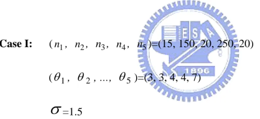
(11223). The box plot and the related statistics for the simulated data are given in
Figure 3.1 and Table 3.1.
Table 3.1. The sample mean, standard deviation, and count for each tool for the simulated data in Case I.
Tool Mean Std Count
T1 2.78 1.58 15
T2 2.88 1.54 150
T3 3.78 1.5 20
T4 3.79 1.55 200
T1 T2 T3 T4 T5 cat -2 0 2 4 6 8 10 da ta
Figure 3.1. Box plots by tools for the simulated data in Case I.
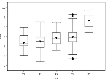
We apply the TCP method to the simulated data in Case I by setting the
tolerance to be 1. The three convergence plots, including v.s. , v.s.
, and v.s. , are displayed in Figure 3.2. We collect the partition
results from the last 10,000 iterations to estimate the posterior distribution of the
partition. The estimated posterior distribution for the partition is given in Figure 3.3.
The correct partition (denoted as (11223)) is the mode of the estimated posterior
distribution with the probability 0.49. From this simulation, we found that the impact
of unbalanced data is very limited.
^ V ^ c W ^ m B ^ c mW B ^ m W ^ c mW W
(a) 0 100 200 300 400 10 20 30 40 (b) 0 100 200 300 400 10 20 30 40 (c) 0 100 200 300 400 10 20 30 40
Figure 3.2. Convergence assessment plots for the simulated data in Case I :
(a) V^ vs. , (b) vs. , and (c) vs. ^ c W ^ m W ^ c mW W ^ m B ^ c mW B
Figure 3.3. Estimated posterior distribution of partition for the simulated data in Case I (and the partition with probability less than 0.005 is not shown).
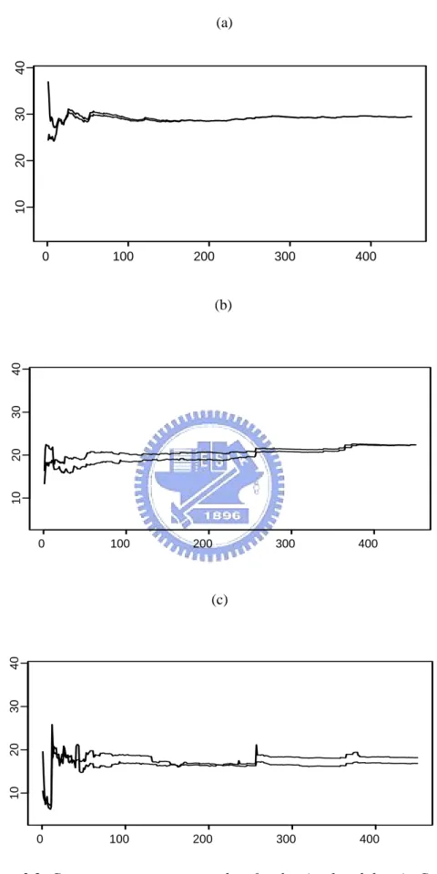
Table 3.2. Partitioning results with respect to different values of cost complexity in the CART model for the simulated data in Case I.
Partitioning result Cost-complexity (1,2,3,4,5) 0 (1,1,2,2,3) 1 (1,1,1,1,2) 90 | T1 T2 T3 T4 T5
We also analyze the same data by the CART method for comparison which is
implemented by the S-Plus functions of tree and prune.tree [46]. The complete tree
result is given in Figure 3.4. and the best partitioning results with respect to different
cost-complexities are given in Table 3.2. According to Table 3.2, one should select a
correct cost-complexity to get reasonable tree results when applying the CART
method. However, it is hard to link the cost complexity with the concept of tolerance
control in engineering. For this reason, the TCP method is much easier for engineers
to use in the connections with engineering tolerance controls.
Case II: (n1, n2, n ,3 n4, n5)=(20, 40, 80, 160, 320)
(
θ
1,θ
2 , …,θ
5)=(5, 3, 5, 3, 3)σ
=1.Similar to Case I, the box plots by tools and the related statistics for the simulated data
are given in Figure 3.5 and Table 3.3. There true partition among 5 tools is denoted as (12122).
By applying TCP method with tolerance =1 and under similar setups as those in Case I, the
estimated posterior distribution for the partition is given in Figure 3.6 and the correct partition
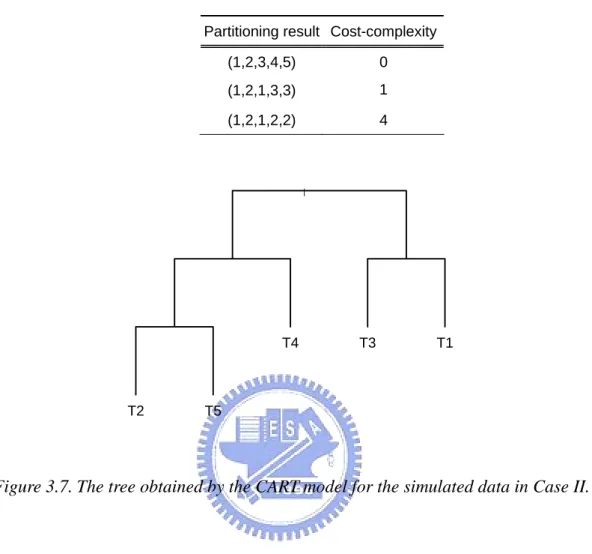
is the posterior mode with probability 0.71. For the same data, the complete tree resulted by
CART is given in Figure 3.7, and the best partitioning results with respect to different
Table 3.3. The sample mean, standard deviation, and count for each tool for the simulated data in Case II.
Tool Mean Std Count
T1 4.25 0.84 20 T2 2.86 0.94 40 T3 4.12 0.94 80 T4 3.16 1.04 160 T5 2.99 1 320 T 1 T 2 T3 T4 T5 T ool -1 1 3 5 dat a
Figure 3.5. Box plots by tools for the simulated data in Case II.
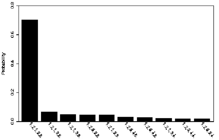
Figure 3.6. Estimated posterior distribution of partition for the simulated data in Case II (the partition with probability less than 0.005 is not shown)
Table 3.4. Partitioning results with respect to different values of cost complexity in the CART model for the simulated data in Case II.
Partitioning result Cost-complexity (1,2,3,4,5) 0 (1,2,1,3,3) 1 (1,2,1,2,2) 4 | T2 T5 T4 T3 T1
Figure 3.7. The tree obtained by the CART model for the simulated data in Case II.
Case III: (n1, n2, n ,3 n4, n5)=(10, 50, 50, 100, 15)
(
θ
1,θ
2 , …,θ
5)=(5, 3, 3, 3, 3)σ
=1The box plot and the related statistics for the simulated data for Case III are given in
Figure 3.8 and Table 3.5. The true partition is denoted as (12222) among 5 tools. Under the
similar setups for the TCP method with tolerance =1, the estimated posterior distribution of the
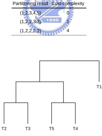
probability 0.71. The complete tree result using CART is given in Figure 3.10, and the best
partitioning results with respect to different cost-complexities are given in Table 3.6 for
comparison.
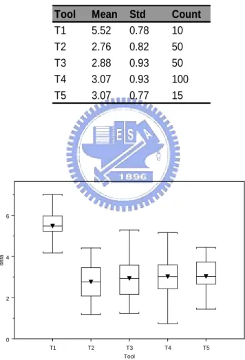
Table 3.5. The sample mean, standard deviation, and count of each tool for the simulated data in Case III.
Tool Mean Std Count
T1 5.52 0.78 10 T2 2.76 0.82 50 T3 2.88 0.93 50 T4 3.07 0.93 100 T5 3.07 0.77 15 T1 T2 T3 T4 T5 Tool 0 2 4 6 da ta
Figure 3.9. Estimated posterior distribution of partition for the simulated data in Case III and (the partition with probability less than 0.005 is not shown).
Table 3.6. Partitioning results with respect to different values of cost complexity in the CART model for the simulated data in Case III.
Partitioning result Cost-complexity (1,2,3,4,5) 0 (1,2,2,3,3) 1 (1,2,2,2,2) 4 | T2 T3 T5 T4 T1
3.2 Sensitivity Analysis with Different Tolerance Controls for
TCP and the Comparison with CART
In the sensitivity analysis, the data are generated from the same model as Case
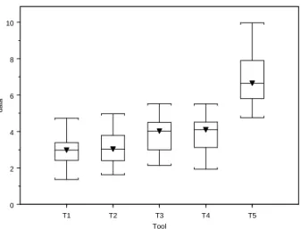
I in Section 3.1, but the number of observations is 30 for each tool and σ is changed
to be 1. The box plots by tools and the related statistics of the simulated data are given
in Figure 3.11 and Table 3.7. The true partition is {(T1, T2), (T3, T4), T5} (denoted as
(11223)). Here, we apply the TCP method with different values of tolerance (= 0.5, 1,
2, 3, 4, 5, 6) to examine its influence on the partition results of the TCP method.
Table 3.7. The sample mean, standard deviation, and count of each tool for the simulated data in Case I with equal sample size.
Tool Mean Std Count
T1 2.90 0.75 30 T2 3.12 0.93 30 T3 3.88 0.99 30 T4 3.86 0.98 30 T5 6.82 1.25 30
T1 T2 T3 T4 T5 Tool 0 2 4 6 8 10 da ta
Figure 3.11. Box plots by tools for the simulated data in Case I with equal sample size.
The partition results under various tolerance levels are given in Table 3.8. The
numbers presented in the table are the posterior probability for each possible partition
and the corresponding estimated error (shown in the parentheses) based on 30
realizations under each tolerance specification. Now, the group means are 3, 3, 4, 4,
and 7 and the within-group standard deviations are 1 in this simulation. When the
tolerance is 0.5 or 1, the target (11223*) will be the most plausible partition because
the between group differences can be as large as 1. When the tolerance is 2, 3, 4, or 5,
the most plausible partition becomes (11112**) because the between group
differences can be as large as 4 and within group standard deviation is 1. When the
tolerance is 6, the most plausible partition moves to (11111***) because the between
group differences are smaller than 6. In the table, we can see that the standard errors
posterior modes. Another interesting phenomenon is that the averages of the posterior
probabilities of three partitions, {11223*}, {11112**} and {11111***}, changes
according to the level of tolerance. Intuitively, tools tends to be merged if the
tolerance is large. For this particular case, the averaged posterior probability for the
partition {11223*} decreases when the tolerance increases. On the other hand, the
averaged posterior probability for the partition {11112**} increases when the
tolerance increases from 0.5 to 3 but decreases when the tolerance increases from 3 to
6. Similarly, the averaged posterior probability for the partition {11111***} increases
when the tolerance increases. Hence, the posterior distributions of the partitions
indeed reflect the levels of tolerance controls. Beside the most plausible partitions, the
posterior distribution also reveals the next plausible partition with the strength of
plausibility (i.e., the posterior probability). This useful information can only be
provided by the Bayesian approach. The results of the sensitivity analysis provide the
evidence that the partitioning results of TCP will be affected by the level of tolerance
controls.
Similarly, based on the same data, the complete tree result using CART is
given in Figure 3.12, and the best partitioning results with respect to different
cost-complexities are given in Table 3.9. It is evident that Table 3.8 contains more
Table 3.8. Averaged posterior probabilities and their standard errors (in the parentheses) for the partition results in the sensitivity analysis for TCP method with
respect to different tolerances.
Tolerance=0.5 Tolerance=1 Tolerance=2 Tolerance=3 Tolerance=4 Tolerance=5 Tolerance=6
11111*** 0(0) 0(0) 0(0) 0.004(0.0051) 0.050(0.0134) 0.239(0.0223) 0.444(0.0181) 11112** 0.005(0.0056) 0.079(0.0176) 0.408(0.0142) 0.495(0.0145) 0.450(0.0157) 0.300(0.0168) 0.159(0.0132) 11122 0(0) 0(0) 0(0) 0.002(0.0014) 0.013(0.0031) 0.027(0.0040) 0.032(0.0042) 11123 0.002(0.0031) 0.018(0.0050) 0.047(0.0048) 0.050(0.0044) 0.046(0.0037) 0.033(0.0024) 0.020(0.0024) 11212 0(0) 0(0) 0(0) 0.003(0.0020) 0.013(0.0038) 0.030(0.0048) 0.033(0.0056) 11213 0.003(0.0038) 0.021(0.0067) 0.052(0.0068) 0.052(0.0064) 0.047(0.0034) 0.032(0.0032) 0.019(0.0029) 11222 0(0) 0(0) 0(0) 0(0) 0.0041(0.0015) 0.012(0.0024) 0.017(0.0031) 11223* 0.683(0.0230) 0.542(0.0321) 0.180(0.0137) 0.093(0.0084) 0.062(0.0060) 0.038(0.0048) 0.020(0.0026) 11234 0.123(0.0130) 0.118(0.0063) 0.057(0.0061) 0.035(0.0042) 0.029(0.0037) 0.019(0.0022) 0.012(0.0018) 12112 0(0) 0(0) 0(0) 0(0) 0.002(0.0011) 0.007(0.0020) 0.011(0.002) 12113 0(0) 0.006(0.0026) 0.026(0.0034) 0.031(0.0029) 0.032(0.0023) 0.024(0.0036) 0.015(0.0018) 12123 0(0) 0.004(0.0016) 0.0233(0.0039) 0.034(0.0037) 0.035(0.0036) 0.026(0.0033) 0.016(0.0027) 12134 0(0) 0.004(0.0015) 0.013(0.0019) 0.016(0.0020) 0.017(0.0020) 0.013(0.0020) 0.009(0.0016) 12213 0(0) 0.003(0.0015) 0.023(0.0029) 0.035(0.0028) 0.037(0.0033) 0.026(0.0035) 0.016(0.0032) 12221 0(0) 0(0) 0(0) 0(0) 0.001(0.0007) 0.006(0.0015) 0.009(0.0018) 12223 0.009(0.0072) 0.028(0.0078) 0.041(0.0059) 0.037(0.0042) 0.034(0.0037) 0.024(0.0033) 0.014(0.0022) 12234 0.004(0.0024) 0.010(0.0027) 0.017(0.0026) 0.017(0.0023) 0.017(0.0017) 0.014(0.0017) 0.009(0.0017) 12314 0.001(0.0008) 0.004(0.0016) 0.013(0.0021) 0.016(0.0022) 0.017(0.0018) 0.013(0.0024) 0.009(0.0017) 12324 0.005(0.0027) 0.011(0.0032) 0.018(0.0021) 0.018(0.0025) 0.017(0.0021) 0.013(0.0025) 0.009(0.0016) 12334 0.096(0.0115) 0.079(0.0080) 0.034(0.0029) 0.0216(0.0025) 0.018(0.0027) 0.013(0.002) 0.008(0.0018) 12345 0.070(0.0092) 0.073(0.0055) 0.047(0.0048) 0.039(0.0038) 0.040(0.0037) 0.031(0.0038) 0.023(0.0029)
Table 3.9. The different partitioning results with respect to different values of cost complexity in the CART model.
Partitioning result Cost-complexity
(1,2,3,4,5) 0 (1,1,2,2,3) 5 (1,1,1,1,2) 25 | T1 T2 T4 T3 T5
Figure 3.12. A tree obtained by the CART model for the simulated data in the sensitivity analysis.
3.3 Robustness Studies by Balanced Simulation Data with
Mean Shifts
In the semiconductor industry, the tool performance often follows a baseline
distribution (for example, a normal distribution) when the tools are in control. On the
contrary, the mean shifts often occur when the tools are out of control. Therefore,
distribution to verify the robustness of the TCP method subject to non-normal data.
3.3.1 Mean Shifts for Lognormal Distribution
The simulation models are described as follows: yij ~ θj+ Lognormal (0,1),
where i=1,2,…, and j=1,2,…,5, with ( , , , ) = (30, 30, 30, 30, 30),
(
j
n n1 n2 n ,3 n4 n5
1
θ ,θ ,…, 2 θ5)=(0, 0, 3, 3, 7). In this experiment, there are 3 groups in 5 tools and the true partition is {(T1, T2), (T3, T4), T5} (denoted as, (1,1,2,2,3)). The box plots
by tools and the related statistics for the simulated data are given in Figure 3.13 and
Table 3.10.
Table 3.10. The sample mean, standard deviation, and count for each tool for the simulated lognormal data in the robustness study.
Tool Mean Std Count
T1 1.51 1.23 30 T2 1.21 1.22 30 T3 4.24 1.63 30 T4 4.45 1.27 30 T5 8.59 1.98 30
T 1 T 2 T 3 T 4 T 5 T o ol 0 5 10 15 data
Figure 3.13. Box plots by tools for the simulated lognormal data in the robustness study.
We apply the TCP methods with tolerance =1 to get the posterior distribution of partitions given in Figure 3.14. The true partition {(T1, T2), (T3, T4), T5} (denoted as, (1,1,2,2,3)) is the posterior mode with the probability 0.7226. For this experiment, we still get correct partition result although the simulated data violate the normal assumption in the TCP method.
Figure 3.14. Estimated posterior distribution of partition for the lognormal data in the robustness study (the partition with probability less than 0.005 is not shown)
3.3.2 Mean Shifts for t Distribution
The simulation models are described as follows:
ij
y ~ θj+ (t distribution with the degrees of freedom 5),
where i=1,2,…, and j=1,2,…,5, with ( , , , ) = (30, 30, 30, 30, 30),
(
j
n n1 n2 n ,3 n4 n5
1
θ ,θ ,…, 2 θ5)=(3, 3, 4, 4, 7). There are 3 groups in 5 tools and the true partition is {(T1, T2), (T3, T4), T5} (denoted as, (1,1,2,2,3)). The box plots by tools and the
related statistics for the simulated data are given in Figure 3.15 and Table 3.11. Using
the TCP methods with tolerance =1, the posterior distribution of partition for this
t-distributed data set is obtained in Figure 3.16 and the posterior mode is still the
correct partition {(T1, T2), (T3, T4), T5} (denoted as, (1,1,2,2,3)) with the probability
0.70364. Again, the TCP method gives a good partition result even when the data are
not normal with mean shifts.
Table 3.11. The sample mean, standard deviation, and count for each tool for the simulated t-distributed data in the robustness study.
Tool Mean Std Count
T1 2.81 1.56 30
T2 3.09 1.17 30
T3 4.21 0.98 30
T4 4.05 1.4 30
T1 T2 T3 T4 T5 To o l - 5 - 1 3 7 dat a
Figure 3.15. Box plots by tools for the simulated t-distributed data in the robustness study.
Figure 3.16. Estimated posterior distribution of partition for the t-distributed data in the robustness study (the partition with probability less than 0.005 is not shown)