保險公司因應死亡率風險之避險策略 - 政大學術集成

全文

(1)國立政治大學風險管理與保險研究所碩士學位論文指導教授 : 黃泓智博士楊曉文博士. 立. 政治大. ‧ 國. 學. 保險公司因應死亡率風險之避險策略. ‧. Hedging Strategy against Mortality Risk for Insurance. y. sit. io. n. al. er. Nat. Company. Ch. engchi. i n U. v. 研究生 : 莊晉國撰. 中華民國一百零一年七月 I.

(2) 中文摘要本篇論文主要討論在死亡率改善不確定性之下的避險策略。當保險公司負債面的人壽保單是比年金商品來得多的時候，公司會處於死亡率的風險之下。我們假設死亡率和利率都是隨機的情況，部分的死亡率風險可以經由自然避險而消除，而剩下的死亡率風險和利率風險則由零息債券和保單貼現商品來達到最適避險效果。我們考慮 mean variance、VaR 和 CTE 當成目標函數時的避險策略，其中在 mean variance 的最適避險策略可以導出公式解。由數值結果我們可以得知保單貼現的確是死亡率風險的有效避險工具。關鍵字: 死亡率風險、Lee Carter model, CIR model, Maximum Entropy principle, Value at risk, Conditional tail expectation, Karush-Kuhn-Tucker.. 立. 政治大. ‧. ‧ 國. 學. n. er. io. sit. y. Nat. al. Ch. engchi. II. i n U. v.

(3) Hedging Strategy against Mortality Risk for Insurance Company Abstract This paper proposes hedging strategies to deal with the uncertainty of mortality improvement. When insurance company has more life insurance contracts than annuities in the liability, it will be under the exposure of mortality risk. We assume both mortality and interest rate risk are stochastic. Part of mortality risk is eliminated. 政治大. by natural hedging and the remaining mortality risk and interest rate risk will be. 立. optimally hedged by zero coupon bond and life settlement contract. We consider the. ‧ 國. 學. hedging strategies with objective functions of mean variance, value at risk and conditional tail expectation. The closed-form optimal hedging formula for mean. ‧. variance assumption is derived, and the numerical result show the life settlement is. al. y. er. io. sit. Nat. indeed a effective hedging instrument against mortality risk.. n. Key words: Mortality risk, Lee Carter model, CIR model, Maximum Entropy principal. Value at risk, Conditional tail expectation, Karush-Kuhn-Tucker.. Ch. engchi. III. i n U. v.

(4) Contents 中文摘要 ....................................................................................................................................... II ABSTRACT ......................................................................................................................................III CONTENTS..................................................................................................................................... IV LIST OF TABLES ............................................................................................................................... V LIST OF FIGURES ............................................................................................................................ VI 1.INTRODUCTION ............................................................................................................................ 1 2.MODELS SETTING ......................................................................................................................... 2 2.1 INTEREST RATE AND MORTALITY RATE MODEL ............................................................................................ 2. 治政大 2.3.A ................................................................................................................ 6 立 3.HEDGING APPROACHES ................................................................................................................ 8. 2.2.THE PROFIT FUNCTION ......................................................................................................................... 4 DJUSTING MORTALITY TABLE. ‧ 國. 學. 4.NUMERICAL EXAMPLES .............................................................................................................. 11 5.CONCLUSIONS ............................................................................................................................ 22. ‧. REFERENCE: ................................................................................................................................... 24. sit. y. Nat. APPENDIX: .................................................................................................................................... 26. io. er. 1.KARUSH-KUHN-TUCKER (KKT) OPTIMALITY CONDITIONS: ............................................................................ 26 2.SOLUTION OF THE OPTIMAL HEDGING PROBLEM ......................................................................................... 26. n. al. Ch. engchi. IV. i n U. v.

(5) List of Tables TABLE 1: ASSETS AND LIABILITIES ................................................................................................... 12 TABLE 2: MEAN OF PROFIT FUNCTIONS .......................................................................................... 14 TABLE 3: COVARIANCE MATRIX OF PROFIT FUNCTIONS .................................................................. 14 TABLE 4 OPTIMAL HEDGING STRATEGIES ........................................................................................ 15 TABLE 5 OPTIMAL HEDGING STRATEGIES ........................................................................................ 20. 立. 政治大. ‧. ‧ 國. 學. n. er. io. sit. y. Nat. al. Ch. engchi. V. i n U. v.

(6) List of Figures FIGURE 1: THE PROFIT FUNCTIONS ON THE LIABILITY SIDE ............................................................. 12 FIGURE 2: THE PROFIT FUNCTIONS ON THE ASSET SIDE .................................................................. 13 FIGURE 3: HEDGING EFFECTIVENESS WITH OBJECTIVE FUNCTION MV Θ = 1 ................................. 16 FIGURE 4: HEDGING EFFECTIVENESS WITH OBJECTIVE FUNCTION MV Θ = 2 ................................. 16 FIGURE 5: HEDGING EFFECTIVENESS WITH OBJECTIVE FUNCTION VAR............................................ 17 FIGURE 6: HEDGING EFFECTIVENESS WITH OBJECTIVE FUNCTION CTE ............................................ 17 FIGURE 8: THE PROFIT FUNCTIONS ON THE ASSET SIDE .................................................................. 19. 政治大 FIGURE 10: HEDGING EFFECTIVENESS WITH OBJECTIVE FUNCTION MV Θ = 2 ............................... 21 立. FIGURE 9: HEDGING EFFECTIVENESS WITH OBJECTIVE FUNCTION MV Θ = 1 ................................. 20 FIGURE 11: HEDGING EFFECTIVENESS WITH OBJECTIVE FUNCTION VAR.......................................... 21. ‧ 國. 學. FIGURE 12: HEDGING EFFECTIVENESS WITH OBJECTIVE FUNCTION CTE .......................................... 22. ‧. n. er. io. sit. y. Nat. al. Ch. engchi. VI. i n U. v.

(7) 1.Introduction Life insurance companies are under the exposures of both longevity and mortality risk due to uncertainty of the mortality improvement. Recent researches and observations prove the significant improvement on the mortality rate of populations around the world. On the other hand, some pandemic diseases and catastrophic natural disaster also frequently cause mortality rate to rise unexpectedly. In order to transfer mortality risk, the insurance companies are seeking alternative hedging instruments. Other hedging instruments such as longevity bonds, longevity swap, q-forward are also. 政治大 longevity risk through capital 立market. For example, Blake, D et al.( 2001) discussed discussed the feasibility of providing solution for transferring the mortality or. ‧ 國. 學. how the survivor bond can hedge the mortality risk, and Dowd, K et al.(2006) introduced survivor swap as a hedging instrument for hedging longevity/mortality. ‧. risk.. sit. y. Nat. Another hedging strategy can be implemented by adjusting the mix of life insurance. al. er. io. and annuity in the liability called natural hedging. Cox, S et al.(2007) proposed using. v. n. natural hedging to stabilize the cash flow of aggregate liability. Wang, J.L et al.(2010). Ch. engchi. i n U. and Tsai, J.T. et al.(2010) investigated the optimal product mix of life insurance and annuity to naturally hedge the longevity and mortality risk. However, to adjust the product mix of life insurance and annuity in the liability to optimal condition is too difficult to implement in practice, controlling the distribution channel of insurance product is too costly to hedge the mortality or longevity risk. But we still cannot ignore the effect of natural hedging even it may not be able to achieve the optimal condition. In this paper, the hedging strategy is to reduce the natural hedged risks by incorporating the hedging instrument. Life settlement(senior life settlement) is a transaction that individuals aged 65 or above can sell their insurance policy to the 1.

(8) investors in the secondary market, the investor will be responsible for paying the premium of this policy and have the right to get the insurance benefit when the insured of this policy is dead. The market for this kind of transactions is fast growing. Life settlement transaction can be a win-win situation for both investors and policyholders. The policyholders can sell their insurance policy with higher price than surrender value, the investors can obtain a relatively low volatility asset which is uncorrelated to the financial asset in the capital market. Because the payoff of life settlement is positive related to the mortality rate, it can be regarded as a hedging vehicle against the mortality risk for insurance company.. 2.Models setting. 立. 政治大. ‧ 國. 學. 2.1 Interest rate and mortality rate model. We focus on two type of risks: interest rate risk and mortality risk. These are two main. ‧. risks affecting the value of insurance products. We assume the interest rate dynamic. sit. y. Nat. following CIR interest rate model(Cox, J. C. et al.(1985)). Under risk neutral measure. al. er. io. Q, the stochastic differential equation of CIR model can be written as. v. n. dr(t) = a�b − r(t)�dt + σ�r(t)dW Q (t). Ch. engchi. i n U. provided 2ab ≥ σ2 , where the coefficient a represents the speed of mean reverting, b is the long-term average interest rate level and σ describes the volatility of interest rate. Assume the market price of risk is of the following form λ(t) = λ�r(t). then the Radon-Nikodym derivatives is. Therefore. t 1 t 2 dQ P � = e∫0 λ�r(u)dW (u)−2 ∫0 λ r(u)du dP Ft. dW Q (t) = dW P (t) − λ�r(t)dt 2.

(9) Under the real-world probability measure P dr(t) = [ab − (a + λσ)r(t)]dt + σ�r(t)dW P (t). = (a + λσ) �. ab − r(t)� dt + σ�r(t)dW P (t) a + λσ. The bond price formula under CIR interest rate model is. where. P(t, T) = A(T − t)e−B(T−t)r(t). and. 2(eγx − 1) B(x) = (γ + a)(eγx − 1) + 2γ. 立. ‧ 國. (a+γ). x 2. (γ + a)(eγx − 1) + 2γ. �. 2ab σ2. ‧. γ = �a2 + 2σ2. 學. A(x) = �. 政治大 2γe. We use Lee Carter model (Lee, R.D et al.(1992)) to model the future mortality. sit. y. Nat. improvement. Although there are many newly developed models providing better. al. er. io. prediction performance than Lee Cater model, Lee Carter model still has attractive. v. n. properties including easy model structure and acceptable prediction errors. Moreover,. Ch. engchi. i n U. we can extend the univariate mortality model to mutlivariate model by giving the correlated structures of k t ′s. For i-th population we can represent the mortality model as. (i). (i). (i). ln�mx,t � = αx + β(i) k x t. Furthermore, we adopt multivariate random walk model to describe the correlated (i). dynamics of all k t 's, which means we can use VAR with lags 0 to model the first (i). difference of k t 's.. 3.

(10) (1) ε1 ⎛Δk t ⎞ μ1 1 ⎜ (2) ⎟ ⎛μ ⎞ ε2 ⎜Δk t ⎟ = ⎜ 2 ⎟ + Σ2 �ε3 � μ3 ⎜Δk (3) ⎟ ε4 t ⎝μ4 ⎠ (4) ⎝Δk t ⎠. 1. where Σ2 is the Cholesky decomposition of covariance matrix Σ and ε1 , ε2 , ε3 and ε4 are four identical and independent standard normal random variables.. 2.2.The profit function. Our goal is to construct the asset portfolio to hedge the interest rate risk and mortality. 政治大 insured and annuitants of different 立 ages and genders. On the asset side, to hedge the. risk in the liability. On the liability side, we consider life contracts and annuities with. ‧ 國. 學. interest rate risk and mortality risk, we choose zero coupon bonds with different maturities and life settlement with insured of different ages and genders as the. ‧. hedging instruments.. sit. y. Nat. When insurance company calculate price of their insurance product including life. al. er. io. contracts and annuities, they always use static reference mortality table instead of. v. n. dynamic stochastic mortality rate. Since the static reference mortality table can not. Ch. engchi. i n U. reflect the impact of uncertain mortality improvement on the price of insurance product. We define the profit function of life contracts or annuities as the difference between actuarial present value calculated by the cohort dynamic mortality rates and actuarial present value calculated by the reference static mortality rate. Since the dynamic mortality rates are stochastic, the profit function is a random variable. We define the notation of profit function of female annuity product by fa fa fa fa πfa �x, rt , mfa x,t � = Vactual �x, rt , mx,t � − Vreference �x, rt , mx,t �. fa where Vcohort is the stochastic actuarial present value calculated by using dynamic. fa cohort mortality rates, Vperiod is the actuarial present value calculated by using static. 4.

(11) reference mortality rates. x denotes age ,rt represents the interest rate and mfa x,t is the. force of mortality for population in female annuity.. Similarly, the profit function for male annuity, female life and male life can be written accordingly.. ma ma ma ma πma �x, rt , mma x,t � = Vactual �x, rt , mx,t � − Vreference �x, rt , mx,t � �l �l π�l �x, rt , m�lx,t � = Vactual �x, rt , m�lx,t � − Vreference �x, rt , m�lx,t �. 政治大 �x, r , m � − V. ml πml �x, rt , mml x,t � = Vactual. 立. t. ml x,t. ml ml reference �x, rt , mx,t �. The profit function of life settlement is the stochastic present value of cash flow. ‧ 國. 學. generated by life settlement minus the cost of buying life settlement, here we assume. ‧. the price of life settlement is determined by the suggested life expectancy of the. y. Nat. insured who sells the life settlement of his/her life insurance contract. Therefore the. ET. er. io. sit. cost of buying life settlement with benefit 1 is. n. a lV� S�x, rt, mx,t� = � 1 i v 1 + rin Ch i=1 engchi U. where ri is the interest rate in year i, ET is the life expectancy suggested by the. medical profession. Then the profit function of life settlement can be defined by the same concept as � S (x, rt ) πS �x, rt , mx,t � = V S �x, rt , mSx,t � − V. where V S �x, rt , mLm,t � is the stochastic present value of cash flow generated by life settlement.. The definition of the profit function of zero coupon bond with face value 1 and maturity T is straightforward.. 5.

(12) πP (rt , T) =. 1. ∏Ti=1(1. + ri ). − P(rt , T). where P(rt , T) is the bond price calculated by using the closed form bond price formula of CIR model.. 2.3.Adjusting mortality table Without the mortality rate for the insured selling life settlement, we will not be able to analyze the distribution of profit function for life settlement. The available information about the insured sold life settlement is the age and life expectancy. Maximum entropy principle provide a reasonable and feasible methodology to adjust. 政治大 obtained information such 立 as life expectancy, variance, median...etc . For example,. the "standard" mortality rates into a adjusted mortality rates by incorporating newly. ‧ 國. 學. Kogure., A. et al.(2010), Johnny Siu-Hang Li et al.(2010) and Johnny Siu-Hang Li et al.(2011) applied maximum entropy principle to change the physical probability. ‧. measure to the objective probability measure for pricing mortality linked derivatives.. sit. y. Nat. We will applied the method in Brockett, P. L. (1991) to construct the life time. al. er. io. distribution of life settlement seller.. n. Let K(x) be the curtate life time of (x). Ch. engchi. i n U. v. According to standard life table the probability mass function of K(x) is (g 0 , g1 , … , g ω−x ). where g i = Pr (K(x) = i). We want to find adjusted mortality table with curtate life time of (x) as (f0 , f1 , … , fω−x ). s. t � fk = 1 and � kfk = ET k. k. where fi = Pr (K(x) = i) under adjusted mortality table and ET is the expectation of lifetime based on newly obtained information.. 6.

(13) To find the adjusted distribution of life time we have to solve the following optimization problem that minimizes the Kullback–Leibler information(Kullback, S et al.(1951)) min � 𝑓𝑘 ln ( fk. subject to. 𝑘. 𝑓𝑘 ) 𝑔𝑘. � fk = 1 k. and. � kfk = ET. 政治大 The solution can be obtained by Lagrange multiplier method. First we consider the 立 k. 學. ‧ 國. Lagrangian function. fk L(f, β) = � fk ln � � − β0 �1 − � fk � − β1 �ET − � fk � gk k. ‧. k. k. y. sit. io. f. er. of equations.. Nat. we need to solve ∇L(f, β) = 0, which is equivalently to solving the following system. n. k � � + 1 + β0 + kβ1 = 0 a⎧ln iv l gk ⎪ ⎪ C n h−1e+n� g cfk h= i0 U. ⎨ ⎪ ⎪ ⎩. −ET + � kfk = 0. ⇒ fk = g k e−1−β0 −kβ1. where β0 and β1 are solution of. k. k. k = 0,1, … , n(= ω − x). ⎧ � g k e−1−β0 −kβ1 = 1 ⎪ k. or equivalently. ⎨� kg k e−1−β0 −kβ1 = ET ⎪ ⎩ k. 7.

(14) min �� 𝑔𝑘 𝑒 −𝛽0 −1−𝛽1 𝑘 � + 𝛽0 + (𝐸𝑇)𝛽1 β0 ,β1. 𝑘. 3.Hedging Approaches As defining the profit function of assets and liabilities, we then define the profit function of the surplus to be the profit function of assets minus profit function of liabilities. nB. nS. i=1. i. π(t) = � Ni πB (rt , Ti ) + � Mi πS �xi , rt , mSm,t � − � ci�l π�l �xi , rt , m�lx,t �. 政治大. i. fa fa fa − � ciml πml �xi , rt , mml x,t � − � ci π �x i , rt , mx,t � i. 立. − � cima πma �xi , rt , mma x,t �. i. ‧ 國. 學. i. where ci�l , ciml are female life and male life insurance benefit for the i-th insured. cifa ,. y. Nat. annuitant.. ‧. cima are female annuity and male annuity annual payment amount for the i-th. er. io. sit. The insurance company need to manage the profit function of surplus. The mean variance optimization problem will be. al. n. v i n C h 𝐸[𝜋(𝑡)] − 𝜃𝑉𝑎𝑟[𝜋(𝑡)] max N ,…,N ,M ,…,M engchi U. subject to. 1. nB. 1. nS. Ni , Mj ≥ 0 ∀i, j. and nB. nS. i=1. i. � S �xi , rt , mSx,t � � Ni P(rt , Ti ) + � Mi V. fa ma ma ma = � cifa Vperiod �xi , rt , mfa x,t � + � ci Vperiod �xi , rt , mx,t � i. i. �l ml + � ci�l Vperiod �xi , rt , m�lx,t � + � ciml Vperiod �xi , rt , mml x,t � i. i. The first constraint is to avoid short position of assets and the second constraint 8.

(15) indicates the budget constraint. Let fa ma ma ma L = � cifa Vperiod �xi , rt , mfa x,t � + � ci Vperiod �xi , rt , mx,t � i. i. �l ml + � ci�l Vperiod �xi , rt , m�lx,t � + � ciml Vperiod �xi , rt , mml x,t � i. Then the budget constraint can be rewritten as nB. nS. i=1. i. i. � S �xi , rt , mSx,t � V B(rt , Ti ) � Ni + � Mi =1 L L. 政治大. This optimization problem includes equality constraints and inequality constraints, the. 立. 學. ‧ 國. Karush-Kuhn-Tucker (KKT) optimality conditions(Kuhn et al.(1951)) in appendix 1 provide a method to solve this problem analytically. ′. ‧. Let u = �M1 , … , MnS , NnS+1 , … , NnB +nS � = (u1 , … , un )′ be the units column vectors,. y. Nat. the first nS components are the units we need to buy life settlements with different. sit. er. io. ages, gender and life expectancies and the last nB components are the units we need to buy bonds with different maturities.. n. al. Ch. Our target is to solve the problem:. engchi. i n U. Σ u max �[m′ , m � ] � � − θ[u′ , −1] � 11 −1 Σ u 21. s. t. u′ a = 1 and u′ ≥ 0. v. Σ12 u � � �� Σ22 −1. where m is the n by 1 mean column vectors of profit function of all the assets, m � is. the sum of expected value of profit function of all liabilities. Σ is the (n+1)*(n+1) covariance matrix of all assets and liabilities, we can decompose Σ into 4 sub-matrices �. Σ11 Σ21. Σ12 � Σ22. Σ11 is n*n matrix represent covariance matrix of assets. Σ22 is 1*1 matrix equaling 9.

(16) to the variance of sum of all liabilities. And B(rt , T1 ) ⎡ ⎤ L ⎢ ⎥ ⋮ ⎢ ⎥ ⎢ B�rt , TNB � ⎥ ⎢ ⎥ L a=⎢ S S � �x1 , rt , mx,t � ⎥ V ⎢ ⎥ L ⎢ ⎥ ⋮ ⎢ ⎥ � S �xN , rt , mSx,t �⎥ ⎢V S ⎣ ⎦ L. Denote. Σ u � + θ[u′ , −1] � 11 −1 Σ21. Σ u �� 治 Σ −1 政大 = −m u + 立m� + θ[u Σ u − Σ u − u Σ + Σ ] f(u) = −[m′ , m �]� ′. ′. 21. ′. 12. ‧ 國. � + θ[u′ Σ11 u − 2u′ Σ12 + Σ22 ] = −m′ u + m. Our optimization problem becomes. sit. a l 1 −1 v −1 i (μ Σ + m − λa) + Σ Σ n 2θC 11 h e n g c h i U11 12. n. if ui > 0 ∀𝑖. er. io. where. y. u. s. t. u′ a − 1 = 0 and −u′ ≤ 0. 22. ‧. min f(x). Nat. The optimal solution is. 22. 學. 11. 12. u=. λ=. −1. −1 a′ Σ11 m − 2θ�1 − a′ Σ11 Σ12 � −1. a′ Σ11 a. The detailed derivation of the solution is in appendix 2. Mean variance approach is easy to implement and has good properties such as closed-form optimal allocation formula, however using first two moments to determine hedging strategies may be too simple to capture the characteristics of profit function. We consider further objective functions such as value at risk(VaR) and 10.

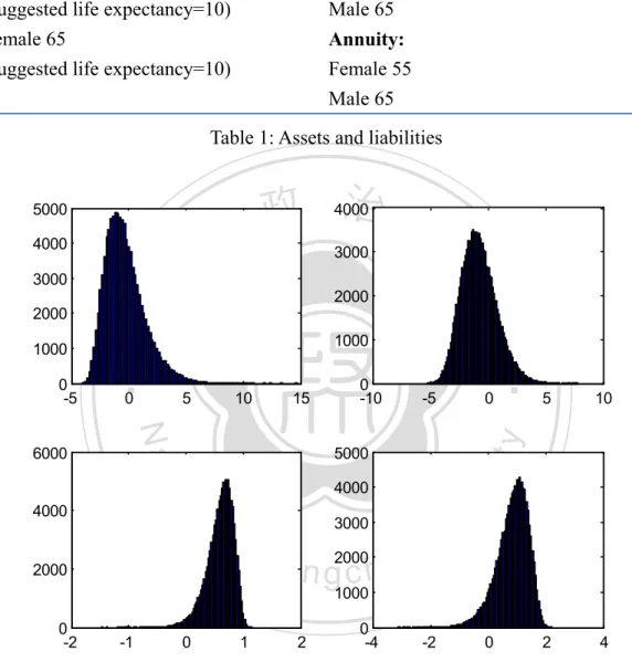
(17) conditional tail expectation(CTE) to offer a comparative hedging performance to the mean variance approach. Set loss function as negative of profit function, that is L = −π. The definition of VaR could be written as. VaR β (L) = inf{ξ|P(L ≤ ξ) = β}. and we apply the result of Trindade et al.(2007) and Pflug, G. (2000) to obtain the value of CTE by solving the following optimization problem. 政治大. 1 立 E �LI 1−β. 𝑢,𝜉. 𝑛. 1 � [𝑙 − 𝜉]+ 𝑓𝐿 (𝑙)𝑑𝑙� 1 − 𝛽 𝑙∈𝑅. io. 1 1 = min �𝜉 + �[𝑙𝑖 − 𝜉]+ � 𝑢,𝜉 1−𝛽𝑛. n. al. 4.Numerical examples. 𝑖=1. Ch. engchi. y. u. Nat. min 𝐶𝑇𝐸𝛽 (𝐿) = min �𝜉 +. sit. ξ. 1 � [𝑙 − 𝜉]+ 𝑓𝐿 (𝑙)𝑑𝑙� 1 − 𝛽 𝑙∈𝑅. ‧. = min �𝜉 +. �L≥VaRβ (L)� �. er. =. 1 � Lf (l)dl 1 − β L≥VaRβ (L) L. 學. Therefore. ‧ 國. CTEβ (L) =. i n U. v. We first consider the mortality is stochastic and the interest rate is non-stochastic. Therefore the interest rate is assumed to be a constant rate 0.03 in this example, there will be 100,000 generated mortality sample paths for calculating profit function of the liabilities. On the asset side, we choose life settlement of insured aged 65 and with suggested life expectancy 10 for both male and female. On the liability side, we include life contracts of female aged 50 and male aged 65 with benefit payment 100, there are also annuities of female aged 55 and male aged 65 with annual payment 1 in the liability. Table 1 summarizes the assets and liabilities: 11.

(18) Asset. Liability. Life settlement: Male 65 (suggested life expectancy=10) Female 65 (suggested life expectancy=10). Life: (benefit=100) Female 50 Male 65 Annuity: Female 55 Male 65. Table 1: Assets and liabilities. 政治大 4000. 5000. 立. 4000. 10. 0. 5000 4000. al. n. 2000. -5. Ch. 3000. e n g2000 chi. 5. 10. 2. 4. sit. io. 4000. 0 -10. 15. y. 5. Nat. 6000. 0. ‧. 0 -5. 1000. er. 1000. 2000. 學. 2000. ‧ 國. 3000. 3000. i n U. v. 1000. 0 -2. -1. 0. 1. 0 -4. 2. -2. 0. Figure 1: The profit functions on the liability side (top left): Life Female 50, (top right): Life Male 65, (bottom left): Annuity Female 55, (bottom right): Annuity Male 65.. The distribution of profit functions are displayed on Figure 1 and Figure 2. We can discover due to mortality improvement, the expected value of profit function of life 12.

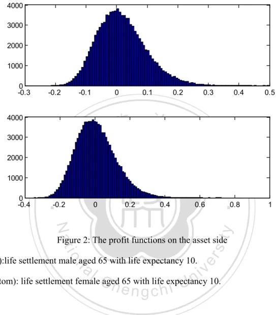
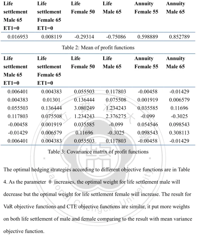
(19) contracts are negative whereas they are positive for annuities. The averaged value of profit function of life settlements are also positive. 4000 3000 2000 1000 0 -0.3. -0.2. -0.1. 0. 4000 3000. 立. 2000. 0.3. 0.4. 0.5. 政治大. ‧ 國 -0.2. 0. 0.2. 0.4. 0.6. ‧. 0 -0.4. 0.2. 學. 1000. 0.1. 1. Nat. y. 0.8. (top):life settlement male aged 65 with life expectancy 10.. al. er. io. sit. Figure 2: The profit functions on the asset side. n. v i n (bottom): life settlement femaleC aged 65 with life expectancy h e n g c h i U 10.. The expected value and covariance matrix of profit functions are shown in Table 2 and Table 3. The life settlements have similar properties to the life insurance contracts, therefore it provide excellent hedging effectiveness against mortality risk from life insurance contracts.. 13.

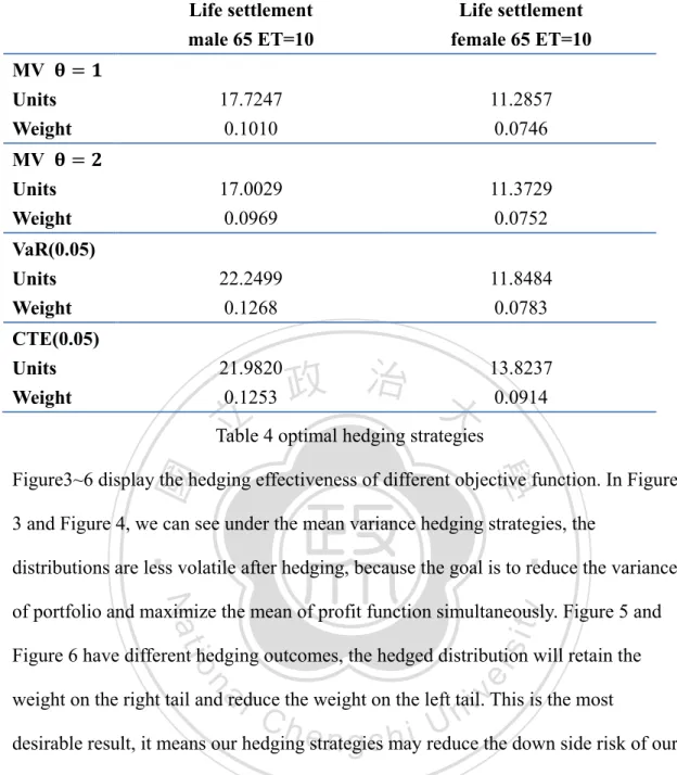
(20) Life settlement Male 65 ET1=0. Life settlement Female 65 ET1=0. Life Female 50. 0.016953. 0.008119. -0.29314. Life Male 65. Annuity Female 55. -0.75086. 0.598889. Annuity Male 65. 0.852789. Table 2: Mean of profit functions Life settlement Male 65 ET1=0. Life settlement Female 65 ET1=0. Life Female 50. 0.006401 0.004383 0.055503 0.117803 -0.00458 -0.01429 0.006401. 0.004383 0.01301 0.136444 0.075508 0.001919 0.006579 0.004383. 0.055503 0.136444 3.080249 1.234243 0.035585 0.11696 0.055503. Annuity Female 55. 0.117803 0.075508 1.234243 2.376275 -0.099 -0.3025 0.117803. 政治大. -0.00458 0.001919 0.035585 -0.099 0.054546 0.098543 -0.00458. 學. ‧ 國. 立. Life Male 65. Annuity Male 65. -0.01429 0.006579 0.11696 -0.3025 0.098543 0.308113 -0.01429. ‧. Table 3: Covariance matrix of profit functions. sit. y. Nat. The optimal hedging strategies according to different objective functions are in Table. al. er. io. 4. As the parameter θ increases, the optimal weight for life settlement male will. v. n. decrease but the optimal weight for life settlement female will increase. The result for. Ch. engchi. i n U. VaR objective functions and CTE objective functions are similar, it put more weights on both life settlement of male and female comparing to the result with mean variance objective function.. 14.

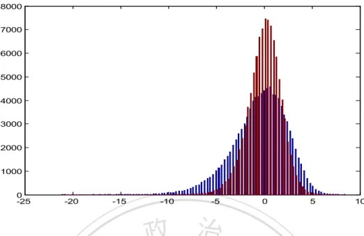
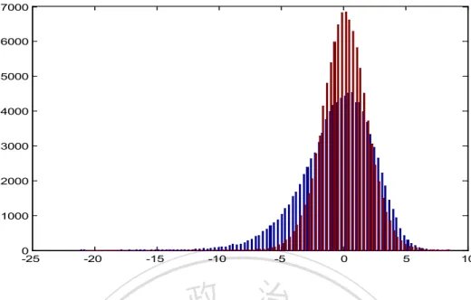
(21) Life settlement male 65 ET=10. Life settlement female 65 ET=10. MV 𝛉 = 𝟏 Units Weight. 17.7247 0.1010. 11.2857 0.0746. MV 𝛉 = 𝟐 Units Weight. 17.0029 0.0969. 11.3729 0.0752. Units Weight. 22.2499 0.1268. 11.8484 0.0783. CTE(0.05) Units Weight. 21.9820 0.1253. VaR(0.05). 立. 政治大. 13.8237 0.0914. Table 4 optimal hedging strategies. ‧ 國. 學. Figure3~6 display the hedging effectiveness of different objective function. In Figure 3 and Figure 4, we can see under the mean variance hedging strategies, the. ‧. distributions are less volatile after hedging, because the goal is to reduce the variance. Nat. sit. y. of portfolio and maximize the mean of profit function simultaneously. Figure 5 and. n. al. er. io. Figure 6 have different hedging outcomes, the hedged distribution will retain the. i n U. v. weight on the right tail and reduce the weight on the left tail. This is the most. Ch. engchi. desirable result, it means our hedging strategies may reduce the down side risk of our portfolio but at the same time it will not harm the opportunity of making profit.. 15.

(22) 8000 7000 6000 5000 4000 3000 2000 1000 0 -25. -5. -10. -15. -20. 5. 0. 10. 政治大. Figure 3: hedging effectiveness with objective function mv θ = 1. 立. (Red):hedged profit function of portfolio. (blue): unhedged profit function of portfolio. 2000. y. sit. 1000 0 -25. er. al. n. 3000. io. 4000. Nat. 5000. ‧. 6000. ‧ 國. 7000. 學. 8000. -20. -15. Ch. engchi -5. -10. i n U 0. v. 5. Figure 4: hedging effectiveness with objective function mv θ = 2. 10. (Red):hedged profit function of portfolio. (blue): unhedged profit function of portfolio. 16.

(23) 7000 6000 5000 4000 3000 2000 1000 0 -25. -20. -15. -10. -5. 0. 5. 10. 政治大. Figure 5: hedging effectiveness with objective function VaR. 立. (Red):hedged profit function of portfolio. (blue): unhedged profit function of portfolio. ‧ 國. y. sit. n. al. er. io. 4000. Nat. 5000. ‧. 6000. 學. 7000. 3000 2000. Ch. engchi. i n U. v. 1000 0 -25. -20. -15. -10. -5. 0. 5. 10. Figure 6: hedging effectiveness with objective function CTE (Red):hedged profit function of portfolio. (blue): unhedged profit function of portfolio Next step, we will discuss the hedging strategies by incorporating both interest risk and mortality risk. The constant interest rate is replaced by100,000 sample paths of interest rate generated according to CIR model with parameters a = 0.2, b = 0.03, 17.

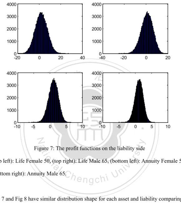
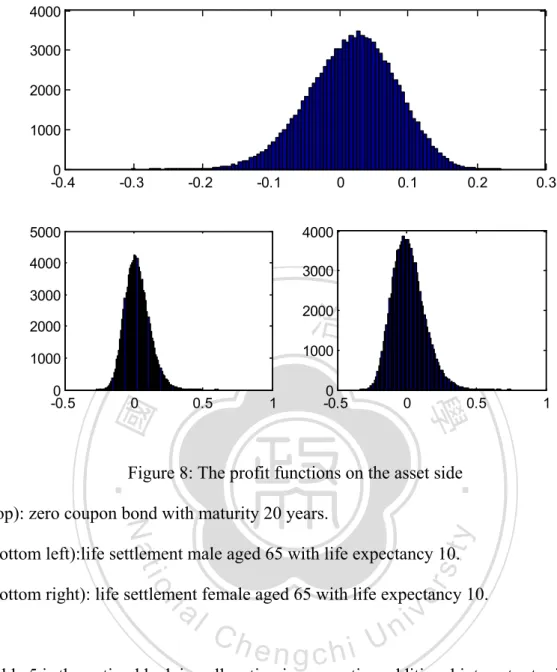
(24) σ = 0.04 and λ = 0.3. Here we include additional asset, zero coupon bond with maturity 20 years to hedge the interest rate risk. 4000. 4000. 3000. 3000. 2000. 2000. 1000. 1000. 0 -20. 0. 20. 0. 20. 4000. 3000. 3000. 立. 1000 0. 5. 0 -10. 10. ‧. -5. 2000. 學. ‧ 國. 2000. 0 -10. -20. 政治大. 4000. 1000. 0 -40. 40. -5. 0. 10. Nat. y. 5. er. io. sit. Figure 7: The profit functions on the liability side. (top left): Life Female 50, (top right): Life Male 65, (bottom left): Annuity Female 55,. n. al. Ch. (bottom right): Annuity Male 65.. engchi. i n U. v. Fig 7 and Fig 8 have similar distribution shape for each asset and liability comparing to the case without interest rate risk but the dispersion is larger due to stochastic interest rate contribute more randomness to the distributions of profit functions.. 18.

(25) 4000 3000 2000 1000 0 -0.4. -0.3. -0.2. -0.1. 0.1. 0.2. 0.3. 0.5. 1. 4000. 5000 4000. 3000. 3000. 政治大 2000. 2000. 1000. 立. 1000 0. ‧ 國. 0.5. 0 -0.5. 1. 0. 學. 0 -0.5. 0. ‧. Figure 8: The profit functions on the asset side. y. Nat. (top): zero coupon bond with maturity 20 years.. er. io. sit. (bottom left):life settlement male aged 65 with life expectancy 10.. (bottom right): life settlement female aged 65 with life expectancy 10.. n. al. Ch. engchi. i n U. v. Table 5 is the optimal hedging allocation incorporating additional interest rate risk, we can observe the large portion of weight is put on the zero coupon bond, hence under our assumption, the interest rate risk dominates the mortality risk. Similarly, as the parameter θ increases, the weight on zero coupon bond and life settlement male. decrease but the weight on life settlement male increases. This result indicates that life settlement female seems has better effect on reducing portfolio variance. While considering the VaR and CTE criterion, we find it put more weight on zero coupon bond and life settlement male. This is quite different form the result of mean variance hedging strategies.. 19.

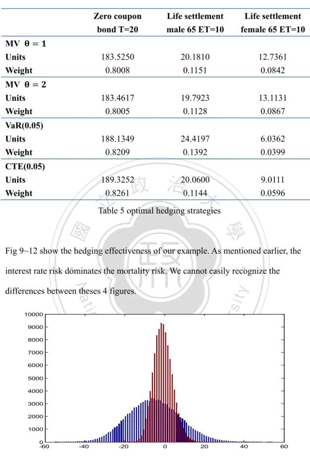
(26) Zero coupon bond T=20. Life settlement male 65 ET=10. Life settlement female 65 ET=10. MV 𝛉 = 𝟏 Units Weight. 183.5250 0.8008. 20.1810 0.1151. 12.7361 0.0842. MV 𝛉 = 𝟐 Units Weight. 183.4617 0.8005. 19.7923 0.1128. 13.1131 0.0867. Units Weight. 188.1349 0.8209. 24.4197 0.1392. 6.0362 0.0399. CTE(0.05) Units Weight. 189.3252 0.8261. VaR(0.05). 20.0600 政治0.1144大. 立. 9.0111 0.0596. Table 5 optimal hedging strategies. ‧ 國. 學. Fig 9~12 show the hedging effectiveness of our example. As mentioned earlier, the. ‧. interest rate risk dominates the mortality risk. We cannot easily recognize the. Nat. sit. n. al. er. io. 10000. y. differences between theses 4 figures.. 9000 8000 7000. Ch. engchi. i n U. v. 6000 5000 4000 3000 2000 1000 0 -60. -40. -20. 0. 20. 40. Figure 9: hedging effectiveness with objective function mv θ = 1. 60. (Red):hedged profit function of portfolio. (blue): unhedged profit function of portfolio. 20.

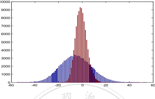
(27) 10000 9000 8000 7000 6000 5000 4000 3000 2000 1000 0 -60. -40. -20. 0. 20. 40. 60. 政治大. Figure 10: hedging effectiveness with objective function mv θ = 2. 立. (Red):hedged profit function of portfolio. (blue): unhedged profit function of portfolio. ‧ 國. y. sit. io. 6000. n. al. er. 7000. Nat. 8000. ‧. 9000. 學. 10000. 5000 4000 3000. Ch. engchi. i n U. v. 2000 1000 0 -60. -40. -20. 0. 20. 40. 60. Figure 11: hedging effectiveness with objective function VaR (Red):hedged profit function of portfolio. (blue): unhedged profit function of portfolio. 21.

(28) 10000 9000 8000 7000 6000 5000 4000 3000 2000 1000 0 -60. 政治大 Figure 12: hedging 立 effectiveness with objective function CTE -40. -20. 0. 20. 40. 60. ‧. ‧ 國. 學. (Red):hedged profit function of portfolio. (blue): unhedged profit function of portfolio. 5.Conclusions. y. Nat. sit. This paper proposes the methodology to hedge mortality risk by life settlement. Using. n. al. er. io. zero coupon bonds and life settlement to hedging the interest rate and mortality risk,. i n U. v. we find the risk on the liability side is effectively reduced. Furthermore we have. Ch. engchi. derived the closed-form optimal solution under mean variance assumption. Hedging strategies with mean variance objective function can adjust the parameter θ to reflect their risk aversion. We also investigate alternative objective function such as VaR and CTE, the result is more attractive for insurance companies, it reduces the downside risk without sacrificing upside profit. Our hedging approaches is flexible. Even we change the interest rate or mortality rate model, the methodology in this paper is still adoptable. This hedging strategy is also applicable in practice for insurance companies which have complicated liabilities structures. Under the mean variance objective function assumption, the larger value θ 22.

(29) is, the more emphasis on reducing variance of portfolio. The mean variance hedging strategy is similar to the strategy of VaR and CTE objective functions, the main target is to control the downside risk. In order to control the downside risk, we not only need to care about the variance but also need to take the mean of portfolio into account. Therefore life settlement can be regard as effective hedging instrument to controlling the mortality risk for insurance companies.. 立. 政治大. ‧. ‧ 國. 學. n. er. io. sit. y. Nat. al. Ch. engchi. 23. i n U. v.

(30) Reference: Blake, D., and Burrows, W., 2001. “Survivor Bonds: Helping to Hedge Mortality Risk”, Journal of Risk and Insurance 68: 339-348. Brockett, P. L., 1991. Information Theoretic Approach to Actuarial Science: A Unification and Extention of Relevant Theory and Applications, Transactions of the Society of Actuaries, 42: 73-115 Cox, J. C., Ingersoll, Jr., J. E., and Ross, S. A., 1985. “A Theory of the Term Structure of Interest Rates”, Econometrica 53: 385-408. Cox, S. H. and Y. Lin, 2007. Natural Hedging of Life and Annuity Mortality Risks,North American Actuarial Journal, 11(3): 1-15.. 政治大. Dowd, K., Blake, D., Cairns, A. J. G., and Dawson, P., 2006. “Survivor Swaps”,. 立. Journal of Risk & Insurance 73: 1-17.. ‧. ‧ 國. 學. Hua Chen, Samuel H. Cox and Zhiqiang Yan, 2010. Hedging Longevity Risk in Life Settlements. Working paper. Johnny Siu-Hang Li, 2010. Pricing longevity risk with the parametric bootstrap: A maximum entropy approach, Insurance: Mathematics and Economics, 47:176-186. Johnny Siu-Hang Li and Andrew Cheuk-Yin NG.,2011. Canonical valuation of mortality-linked securities, The Journal of Risk and Insurance, Vol. 78, No. 4, 853-884 Kogure., A., and Kurachi, Y., 2010. A Bayesian Approach to Pricing Longevity Risk Based on Risk-Neutral Predictive Distributions, Insurance: Mathematics and Economics, 46:162-172.. n. er. io. sit. y. Nat. al. Ch. engchi. i n U. v. Kuhn, H. W.; Tucker, A. W., 1951. "Nonlinear programming". Proceedings of 2nd Berkeley Symposium. Berkeley: University of California press. pp. 481-492. Kullback, S., and R. A. Leibler, 1951. On Information and Sufficiency, Annals of Mathematical Statistics, 22: 79-86. Lee, R.D., Carter, L.R., 1992. Modeling and forecasting US mortality. Journal of the American Statistical Association 87, 659_675. Pflug, G., 2000. Some Remarks on the Value-at-Risk and the Conditional Value-at-Risk. S. Uryasev, ed. Probabilistic Constrained Optimization Methodology and Applications. Kluwer, Dordrecht, The Netherlands, 272–281. 24.

(31) Trindade, A. A., S. Uryasev, A. Shapiro, and G. Zrazhevsky, 2007. Financial Prediction with Constrained Tail Risk. Journal of Banking and Finance 31 3524– 3538. Tsai, J.T., J.L. Wang, and L.Y. Tzeng, 2010. On the optimal product mix in life insurance companies using conditional Value at Risk, Insurance: Mathematics and Economics, 46, 235-241. Wang, J.L., H.C. Huang, S.S. Yang, J.T. Tsai, 2010. An optimal product mix for hedging longevity risk in life insurance companies: The immunization theory approach, The Journal of Risk and Insurance, Vol. 77, No. 2, 473-497.. 立. 政治大. ‧. ‧ 國. 學. n. er. io. sit. y. Nat. al. Ch. engchi. 25. i n U. v.

(32) Appendix: 1.Karush-Kuhn-Tucker (KKT) optimality conditions: Consider the constrained optimization problem: min f(x) x. g j (x) ≤ 0, 𝑗 = 1, … , 𝑚 s. t. � hl (x) = 0, l = 1, … , r. The Lagrangian Function is given by. m. r. j=1. l=1. L(x, µ, λ) = f(x) + � µj g j (x) + � λl hl (x). 政治大 IF x* is an optimal solution of the problem, then there exist Lagrange multipliers µ 立 � µ∗j ∇g j (x ∗ ) j=1. + � λ∗l ∇hl (x ∗ ) = 0 l=1. io. hl (x ∗ ) = 0 ∀ l = 1, … , r µj∗ ≥ 0 ∀ j = 1, … , m. n. al. y. g j (x ∗ ) ≤ 0 ∀ j = 1, … , m. sit. Nat This is the KKT condition. r. er. ‧ 國. +. m. ‧. ∇f(x. ∗). 學. and λ∗ such that. i , mn C h = 0 ∀ j = 1, …U engchi. µ∗j g j (x ∗ ). v. 2.Solution of the optimal hedging problem The Lagrangian function can be written as L(u, μ, λ) = f(u) − μ′ u + λ(u′ a − 1). The KKT conditions imply the following system of equations:. where. ∇f(u) − μ + λa = 0 ∇f(u) =. (1). ∂f(u) = −m + θ[2Σ11 u − 2Σ12 ] ∂u 26. ∗.

(33) u′ a − 1 = 0. (2). μ≥0. (4). −u ≤ 0. (3). μi ui = 0 i = 1, … , N. Case 1: ui > 0 ∀𝑖. (5). (1)=>. −m + θ[2Σ11 u − 2Σ12 ] − μ + λa = 0 1 (μ + m − λa) + Σ12 2θ. 政治大. 1 −1 −1 Σ11 (μ + m − λa) + Σ11 Σ12 2θ. u=. 1 −1 −1 Σ (m − λa) + Σ11 Σ12 2θ 11. ‧ 國. Nat. a′ u = 1. al. 1 ′ −1 −1 a Σ (m − λa) + a′ Σ11 Σ12 = 1 2θ 11. n. ⇒. er. io. 1 −1 −1 (m − λa) + Σ11 ⇒ a′ � Σ11 Σ12 � = 1 2θ −1. ‧. substitute u into (2) we can solve λ easily. (∗). y. 立. From (5), IF ui ≠ 0 ∀ i then μi = 0 ∀ i so we have. 學. u=. sit. ⇒ Σ11 u =. Ch. e−1n g c h i. i n U. v. −1 ⇒ a′ Σ11 m − λa′ Σ11 a = 2θ�1 − a′ Σ11 Σ12 �. λ=. −1. −1 a′ Σ11 m − 2θ�1 − a′ Σ11 Σ12 � −1. a′ Σ11 a. (∗∗). substitute (**) into (*), we get the desired optimal asset allocation. −1. −1 a′ Σ11 m − 2θ�1 − a′ Σ11 Σ12 � 1 −1 −1 u = Σ11 a� + 2Σ11 Σ12 �m − −1 ′ θ a Σ11 a. Case 2:ui = 0 for some i's. suppose there are k u′s being zero say. 27.

(34) u(1) = u(2) = ⋯ = u(k) = 0 {(1), … , (k)} ∈ {1, … , N}. and (1) ≤ (2) ≤ ⋯ ≤ (k). The other u′s are nonzero called. u(1)′ , u(2)′ , … , u(N−k)′. By (5) of KKT condition, we can say μ(1) , … , μ(k) are nonzero, The others are all zero. called μ(1)′ , … , μ(N−k)′. From the expression of u. 1 −1 −1 Σ11 (μ + m − λa) + Σ11 Σ12 2θ. u=. 政治大. Define uA = (u(1) , u(2) , … , u(k) )′,we have. 立. 1 −1 −1 Σ ((1): (k), : )(μ + m − λa) + Σ11 ((1): (k), : )Σ12 2θ 11. ‧ 國. 學. uA = 0 =. −1 here Σ11 ((1): (k), : ) denotes the matrix obtained by picking rows (1), (2),...,(k) from. ‧. −1 Σ11 .. Nat. we also define μA = (μ(1) , … , μ(k) )′, then. y. sit. −1 + Σ11 ((1): (k), : )Σ12 = 0. n. al. er. io. 1 −1 1 −1 λ −1 Σ11 �(1): (k), (1): (k)�μA + Σ11 �(1): (k), : �m − Σ11 �(1): (k), : �a 2θ 2θ 2θ ⇒ =. Ch. −1 Σ11 �(1): (k), (1): (k)�μA. −1 λΣ11 �(1): (k), : �a. ⇒ μA. −. engchi. −1 Σ11 �(1): (k), : �m. i n U. v. −1 − 2θΣ11 ((1): (k), : )Σ12. −1 −1 = Σ11 �(1): (k), (1): (k)��λΣ11 �(1): (k), : �a − Σ11 �(1): (k), : �m −1 − 2θΣ11 ((1): (k), : )Σ12 �. −1 where Σ11 �(1): (k), (1): (k)� means picking rows (1), (2),...,(k) and columns (1), −1 (2),...,(k) from Σ11 to form the new submatrix.. The remaining part is to solve λ. By the (2) of KKT condition, and define aB = (a(1)′ , a(2)′ , … , a(N−k)′ )′ and 28.

(35) uB = (u(1)′ , u(2)′ , … , u(N−k)′ )′. a′B uB = 1. we have. 1 −1 −1 ((1)′ : (N − k)′ , : )(m − λa) + Σ11 ((1)′ : (N − k)′ , : )Σ12 � = 1 a′B � Σ11 2θ. −1 −1 ((1)′ : (N − k)′ , : )(m − λa) = 2θ�1 − a′B Σ11 ((1)′ : (N − k)′ , : )Σ12 � ⇒ a′B Σ11 −1 −1 ((1)′ : (N − k)′ , : )m − 2θ�1 − a′B Σ11 ((1)′ : (N − k)′ , : )Σ12 � a′B Σ11 −1 ((1)′ : (N − k)′ , : )a a′B Σ11. 立. 政治大. 學 ‧. ‧ 國 io. sit. y. Nat. n. al. er. λ=. Ch. engchi. 29. i n U. v.

(36)