以代理人基模型模擬的施與受賽局 - 政大學術集成

全文

(1)國立政治大學理學院應用物理研究所碩士論文 Graduate Institute of Applied Physics, College of Science National Chengchi University Master Thesis. 以代理人基模型模擬的施與受賽局. Donor-Recipient Game. 學. 曾嘉瑤. ‧ y. Nat. Chia-Yao Tseng. er. io. sit. ‧ 國. 政治大 Agent-Based Model Simulation of 立. n. al v 指導教授：馬文忠博士 ni Ch. engchi U. 陳樹衡博士. Advisor: Prof. Wen-Jong Ma Prof. Shu-Heng Chen. 中華民國一○二年七月 July, 2013 1.

(2) Abstract The effects of human cooperation on the societies and on the individuals is an important issue in social science. The dynamics of a model society of individuals with adjustable cooperation strategies and with varying reputations gauged by social norms has been recently proposed [1]. In order to refine the mean-field type analysis, we implement the Agent-based model in computer simulations, where the strategy adjustment of each individual is determined by a social learning procedure. In between consecutive strategy changes, one individual encounters a partner in a. 政治大. Donor-Recipient game, which results in the wealth changes in both parties in form. 立. of cost, punishment or benefit and is followed by a reputation re-assignment to the. ‧ 國. 學. donor, taking into account the strategy of the donor and the reputation of the recipient. The accumulated knowledge of wealth changes from sequences of games. ‧. for all individuals in the society weighs the strategy change transitions. We obtain. Nat. sit. y. some primitive observations on the evolutions of strategies adapted by the. n. al. er. io. individuals of the model society. Using the agent-based models to simulate three. i n U. v. kinds of social norms: Simple social norm (punishment-free social norm), Weakly. Ch. engchi. augmented social norm (punishment-optional social norm) and Strongly augmented social norm (punishment-provoking social norm). We try to compare the outcome of the agent-based model with the solutions of mean-field equation. The two methods are found to have unanimous results: they have the same the primary solution and the main secondary solution; punishment would promote cooperation and social norms in strong penalties exist under the second secondary solution. In contrast to the mean-field scenario, the players in the agent based model update their strategies asynchronously, based on the accumulated knowledge of wealth changes for players adapting each strategy. We distinguish the models of two modules of such i.

(3) knowledge, learned either by simple averages (player-weighted method) or by weighted averages (event-weighted method). In carrying out the zero-temperature analogy of spin-flipping simulation, we obtain some primitive observations on the strategy evolution of the agents. While all solutions of the mean field equations are consistently obtained in the latter case, only the primary solution is found for the former case in each social norm. It is found that a minor stable attractor may survive in the time evolution which are ported by harmonious societies, where all agents are reputed as “good”.. In the time evolution, the competition between strategies may. display the presence of dynamic orbits as the final domain of time evolution.. 立. 政治大. [1] Tongkui Yu, Shu-heng Chen, Honggang Li, "Social Norm, Costly Punishment. ‧ 國. 學. and the Evolution to Cooperation," 17th International Conference on Computing in Economics and Finance.. ‧ y. Nat. io. sit. Keywords：Agent-based model, Donor-Recipient game, Social norms,. n. al. er. Asynchronous, logistic distribution, Boltzmann distribution,. Ch. i n U. zero-temperature simulations, Potts Model.. engchi. ii. v.

(4) 摘要人類合作造成的社會影響與個人影響是社會科學的一個重要問題。最近提出了一個動態可調整的合作策略和不同聲譽的衡量規範的個人社會模型 [1]。為了將平均場分析結果作進一步解析，我們以代理人基模型進行電腦計算模擬。在模型中的每一位代理人實施的策略調整，均由社會學習模式來決定，類似在 Potts 模型下 Metropolis 能量驅動的狀態轉換。在施與受賽局演化模型中，社會由許多代理人組成，每一個代理人會隨機遇到另一個代理人，雙方共同合作，構成捐贈方及受援方的成對組合。在給定捐贈方的策略及受援方的評價後，捐. 政治大. 贈方每一回合遊戲可以採取合作或不合作，與加入懲罰的三種策略。在遊戲試. 立. 驗進行中，根據各種策略已經給定合作的交易成本與收益以及懲罰的成本與損. ‧ 國. 學. 失，在每一回合遊戲進行結束後，捐贈方將被重新給定評價，並且計算全體代. ‧. 理人的財富變化。在連續進行的遊戲中，代理人會根據每個代理人與社會群體的財富變化，產生知識累積的學習模式，作為策略轉換權數的基準。在以類比. y. Nat. io. sit. 於自旋翻換模型於溫度零度的模擬下，我們對此社會模型代理人策略採取的演. n. al. er. 化模式，得到了一些初步觀察的結果。使用代理人基模型模擬三種社會規範：. i n U. v. 簡單社會規範（無懲罰的社會規範），弱懲罰社會規範（允許懲罰的社會規範）. Ch. engchi. 與強懲罰的社會規範（加強懲罰的社會規範）與平均場理論作初步比較。模擬結果得出與原先平均場理論一致的結論：主要解與第一次要解均相同，懲罰將促進合作，並在強懲罰社會規範下存在第二次要解。在代理人基模型的各代理人是以社會學習模式後採取更新策略。社會學習與個人學習的差異在於，每一位代理人賽局累積經驗作為學習的樣本來自於社會全體代理人還是只有自己。在賽局中各代理人的所得與財富將依照代理人在每一回合賽局中的身份與策略產生變動，對此變動計數在分別以兩種模式：簡單平均（人數權重法）與權重平均（事件權重法）計算平均法得出，簡單平均法產生唯一主要解，權重平均法將差異保留，主要解與次要解共存。我們發現 iii.

(5) 代理人基模型中最終狀態的次要解，除了可能以其所有成員都為好人的合諧社會的型式出現外，也可能是以極限軌道而非離散點的新型態出現。. [1] Tongkui Yu, Shu-heng Chen, Honggang Li, "Social Norm, Costly Punishment and the Evolution to Cooperation," 17th International Conference on Computing in Economics and Finance.. 關鍵字：代理人基模型，施與受賽局，社會規範，非同步，羅吉斯分佈，波茲曼分佈，零度模擬，波茨模型。. 立. 政治大. ‧. ‧ 國. 學. n. er. io. sit. y. Nat. al. Ch. engchi. iv. i n U. v.

(6) Table of Content Chapter 1.. Introduction .................................................................................. 1. 1.1. History. .......................................................................................................... 1. 1.2. Motivation. .................................................................................................... 3. 1.3. Method. ......................................................................................................... 5. Chapter 2.. 2.2. Donor-recipient game ................................................................................. 11 2.1.1. Strategies and social norms .............................................................. 13. 2.1.2. Fluctuation and uncertainty.............................................................. 16. 立. 政治大. Evolutionary dynamics of strategies ........................................................... 17. 學. Chapter 3.. ‧ 國. 2.1. Model ......................................................................................... 11. Experimental Results Analysis .................................................. 32. Coarsened social learning versus refined social learning ........................... 33. 3.2. Societies with low strategy switching frequency ........................................ 42. 3.3. Societies with high strategy switching frequency ....................................... 55. 3.4. Discussion ................................................................................................... 87. ‧. 3.1. er. io. sit. y. Nat. al. n. v i n C h ................................................................. Concluding Remarks 93 engchi U. Chapter 4.. Appendix. ....................................................................................................... 95 A.1. Boltzmann distribution............................................................................... 95. A.2 Stable reputation distribution in mean field calculation ............................ 96. A.3. A.2.1. Simple Social Norm (GGBG) ......................................................... 97. A.2.2. Weakly Augmented Social Norm (GGBGBG) ............................. 102. A.2.3. Strongly Augmented Social Norm (GGBBBG) ............................ 104. Fitness of strategies .................................................................................. 106 A.3.1. Simple Social Norm ...................................................................... 107 I.

(7) A.3.2. Weakly Augmented Norm ............................................................. 109. A.3.3. Strongly Augmented Norm ........................................................... 111. Reference .................................................................................................... 113. 立. 政治大. ‧. ‧ 國. 學. n. er. io. sit. y. Nat. al. Ch. engchi. II. i n U. v.

(8) List of Figures. Figure 2.1: Typical social norms with the related ordinary strategies (a. simple, b. weakly augmented and c. strongly augmented) ------------14 Figure 2.2(a): time evolution for agent 47 ------------------------------------------------20 Figure 2.2(b): time evolution for agent 95 ------------------------------------------------20. 政治大. Figure 2.2(c): first switch time earliest ----------------------------------------------------21. 立. Figure 2.2(d): first switch time latest ------------------------------------------------------21. ‧ 國. 學. Figure 2.2(e): final switch time earliest ---------------------------------------------------22. ‧. Figure 2.2(f): final switch time latest ------------------------------------------------------22. y. Nat. n. al. er. io. sit. Figure 2.2(g): switch time interval smallest ----------------------------------------------23. v. Figure 2.2(h): switch time interval largest ------------------------------------------------23. Ch. engchi. i n U. Figure 2.2(i): number of switch time smallest -------------------------------------------24 Figure 2.2(j): number of switch time largest ---------------------------------------------24 Figure 2.3: statistical results of the switch times of strategies -------------------------25 Figure 2.4(a): Flow chart -------------------------------------------------------------------27 Figure 2.4(b): Flow chart -------------------------------------------------------------------28 Figure 2.5: Social learning theory illustration -------------------------------------------30 III.

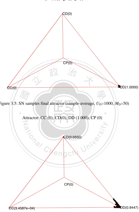
(9) Figure 3.1(a): Population n in one typical experiment ----------------------------------34 Figure 3.1(b): Good reputation g of population in one typical experiment ----------34 Figure 3.2(a): Population n in one typical experiment ----------------------------------35 Figure 3.2(b): Good reputation g of population in one typical experiment ----------35 Figure 3.3(a): Population n in one typical experiment ----------------------------------38 Figure 3.3(b): Good reputation g of population in one typical experiment ----------38. 政治大. Figure 3.4(a): Population n in one typical experiment ----------------------------------39. 立. Figure 3.4(b): Good reputation g of population in one typical experiment ----------39. ‧ 國. 學. Figure 3.5: SN samples final attractor. ‧. (simple-average, UD=1000, MD=50) -----------------------------------------43. y. Nat. n. er. io. al. sit. Figure 3.6: SN samples final attractor. v. (simple-average, UD=10000, MD=50) ---------------------------------------43. Ch. engchi. i n U. Figure 3.7: SN samples final attractor. (weighted-average, UD=1000, MD=50) --------------------------------------45 Figure 3.8: SN samples final attractor (weighted-average, UD=10000, MD=50) ------------------------------------45 Figure 3.9(a): WA samples final attractor basin (simple-average, UD=1000, MD=50) ------------------------------------47 IV.

(10) Figure 3.9(b): WA samples final attractor (simple-average, UD=1000, MD=50) ------------------------------------47 Figure 3.10(a): WA samples final attractor basin (simple-average, UD=10000, MD=50) ---------------------------------48 Figure 3.10(b): WA samples final attractor (simple-average, UD=10000, MD=50) ---------------------------------48. 政治大. Figure 3.11(a): WA samples final attractor basin. 立. (weighted-average, UD=1000, MD=50) --------------------------------49. ‧ 國. 學. Figure 3.11(b): WA samples final attractor. ‧. (weighted-average, UD=1000, MD=50) --------------------------------49. y. Nat. n. er. io. al. sit. Figure 3.12(a): WA samples final attractor basin. v. (weighted-average, UD=10000, MD=50) ------------------------------50. Ch. engchi. i n U. Figure 3.12(b): WA samples final attractor. (weighted-average, UD=10000, MD=50) ------------------------------50 Figure 3.13(a): SA samples final attractor basin (simple-average, UD=1000, MD=50) -----------------------------------51 Figure 3.13(b): SA samples final attractor (simple-average, UD=1000, MD=50) -----------------------------------51 V.

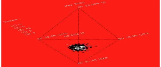
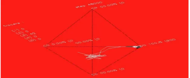
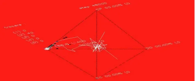
(11) Figure 3.14(a): SA samples final attractor basin (simple-average, UD=10000, MD=50) ----------------------------------52 Figure 3.14(b): SA samples final attractor (simple-average, UD=10000, MD=50) ----------------------------------52 Figure 3.15(a): SA samples final attractor basin (weighted-average, UD=1000, MD=50) --------------------------------53. 政治大. Figure 3.15(b): SA samples final attractor. 立. (weighted-average, UD=1000, MD=50) --------------------------------53. ‧ 國. 學. Figure 3.16(a): SA samples final attractor basin. ‧. (weighted-average, UD=10000, MD=50) ------------------------------54. y. Nat. n. er. io. al. sit. Figure 3.16(b): SA samples final attractor. v. (weighted-average, UD=10000, MD=50) ------------------------------54. Ch. engchi. i n U. Figure 3.17(a): SN samples moving trajectory at step 0 --------------------------------57 Figure 3.17(b): SN samples moving trajectory at step 2000 ---------------------------57 Figure 3.17(c): SN samples moving trajectory at step 4000 ---------------------------57 Figure 3.17(d): SN samples moving trajectory at step 6000 ---------------------------58 Figure 3.17(e): SN samples moving trajectory at step 9000 ---------------------------58 Figure 3.17(f): SN samples moving trajectory at step 12000 --------------------------58 VI.

(12) Figure 3.17(g): SN samples moving trajectory at step 15000 --------------------------59 Figure 3.17(h): SN samples moving trajectory at step 18000 --------------------------59 Figure 3.17(i): SN samples moving trajectory at step 24000 ---------------------------59 Figure 3.17(j): SN samples moving trajectory at step 36000 ---------------------------60 Figure 3.17(k): SN samples moving trajectory at step 48000 --------------------------60 Figure 3.17(l): SN samples moving trajectory at step 60000 ---------------------------60. 政治大. Figure 3.18(a): WA samples moving trajectory at step 0 -------------------------------61. 立. Figure 3.18(b): WA samples moving trajectory at step 2000 --------------------------61. ‧ 國. 學. Figure 3.18(c): WA samples moving trajectory at step 4000 --------------------------61. ‧. Figure 3.18(d): WA samples moving trajectory at step 6000 --------------------------62. y. Nat. n. al. er. io. sit. Figure 3.18(e): WA samples moving trajectory at step 9000 --------------------------62. v. Figure 3.18(f): WA samples moving trajectory at step 12000 -------------------------62. Ch. engchi. i n U. Figure 3.18(g): WA samples moving trajectory at step 15000 ------------------------63 Figure 3.18(h): WA samples moving trajectory at step 18000 ------------------------63 Figure 3.18(i): WA samples moving trajectory at step 24000 -------------------------63 Figure 3.18(j): WA samples moving trajectory at step 36000 -------------------------64 Figure 3.18(k): WA samples moving trajectory at step 48000 ------------------------64 Figure 3.18(l): WA samples moving trajectory at step 60000 -------------------------64 VII.

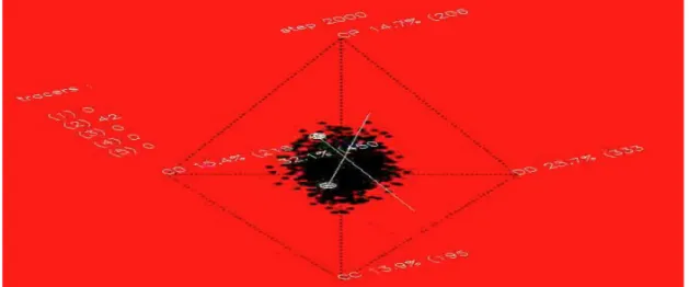
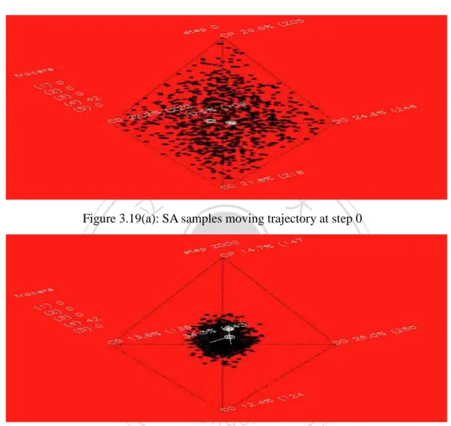
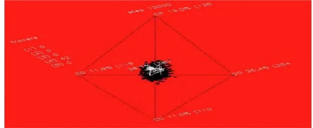
(13) Figure 3.19(a): SA samples moving trajectory at step 0 --------------------------------65 Figure 3.19(b): SA samples moving trajectory at step 2000 ---------------------------65 Figure 3.19(c): SA samples moving trajectory at step 4000 ---------------------------65 Figure 3.19(d): SA samples moving trajectory at step 6000 ---------------------------66 Figure 3.19(e): SA samples moving trajectory at step 9000 ---------------------------66 Figure 3.19(f): SA samples moving trajectory at step 12000 --------------------------66. 政治大. Figure 3.19(g): SA samples moving trajectory at step 15000 --------------------------67. 立. Figure 3.19(h): SA samples moving trajectory at step 18000 --------------------------67. ‧ 國. 學. Figure 3.19(i): SA samples moving trajectory at step 24000 --------------------------67. ‧. Figure 3.19(j): SA samples moving trajectory at step 36000 --------------------------68. y. Nat. n. al. er. io. sit. Figure 3.19(k): SA samples moving trajectory at step 48000 -------------------------68. v. Figure 3.19(l): SA samples moving trajectory at step 60000 --------------------------68. Ch. engchi. i n U. Figure 3.20(a): SN samples moving trajectory at step 0 -------------------------------69 Figure 3.20(b): SN samples moving trajectory at step 200 ----------------------------69 Figure 3.20(c): SN samples moving trajectory at step 300 ----------------------------69 Figure 3.20(d): SN samples moving trajectory at step 400 ----------------------------70 Figure 3.20(e): SN samples moving trajectory at step 500 ----------------------------70 Figure 3.20(f): SN samples moving trajectory at step 600 ----------------------------70 VIII.

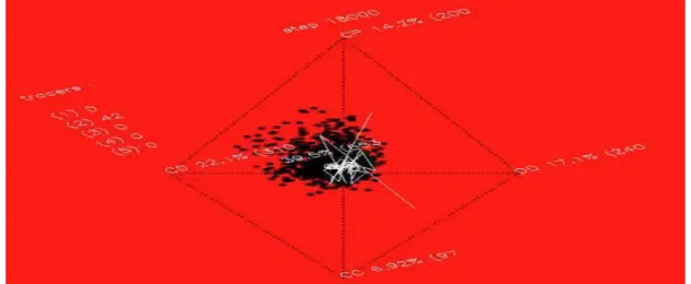
(14) Figure 3.20(g): SN samples moving trajectory at step 700 -----------------------------71 Figure 3.20(h): SN samples moving trajectory at step 800 -----------------------------71 Figure 3.20(i): SN samples moving trajectory at step 1000 ----------------------------71 Figure 3.20(j): SN samples moving trajectory at step 2000 ----------------------------72 Figure 3.20(k): SN samples moving trajectory at step 4000 ---------------------------72 Figure 3.20(l): SN samples moving trajectory at step 6000 ----------------------------72. 政治大. Figure 3.21(a): WA samples moving trajectory at step 0 -------------------------------73. 立. Figure 3.21(b): WA samples moving trajectory at step 200 ----------------------------73. ‧ 國. 學. Figure 3.21(c): WA samples moving trajectory at step 400 ----------------------------73. ‧. Figure 3.21(d): WA samples moving trajectory at step 600 ----------------------------74. y. Nat. n. al. er. io. sit. Figure 3.21(e): WA samples moving trajectory at step 800 ----------------------------74. v. Figure 3.21(f): WA samples moving trajectory at step 1000 ---------------------------74. Ch. engchi. i n U. Figure 3.21(g): WA samples moving trajectory at step 1200 --------------------------75 Figure 3.21(h): WA samples moving trajectory at step 1600 --------------------------75 Figure 3.21(i): WA samples moving trajectory at step 2000 --------------------------75 Figure 3.21(j): WA samples moving trajectory at step 2400 --------------------------76 Figure 3.21(k): WA samples moving trajectory at step 4800 -------------------------76 Figure 3.21(l): WA samples moving trajectory at step 7200 --------------------------76 IX.

(15) Figure 3.22(a): SA samples moving trajectory at step 0 --------------------------------77 Figure 3.22(b): SA samples moving trajectory at step 200 -----------------------------77 Figure 3.22(c): SA samples moving trajectory at step 400 -----------------------------77 Figure 3.22(d): SA samples moving trajectory at step 600 -----------------------------78 Figure 3.22(e): SA samples moving trajectory at step 800 -----------------------------78 Figure 3.22(f): SA samples moving trajectory at step 1000 ----------------------------78. 政治大. Figure 3.22(g): SA samples moving trajectory at step 1200 ---------------------------79. 立. Figure 3.22(h): SA samples moving trajectory at step 1600 ---------------------------79. ‧ 國. 學. Figure 3.22(i): SA samples moving trajectory at step 2000 ----------------------------79. ‧. Figure 3.22(j): SA samples moving trajectory at step 2400 ----------------------------80. y. Nat. n. al. er. io. sit. Figure 3.22(k): SA samples moving trajectory at step 4800 ---------------------------80. v. Figure 3.22(l): SA samples moving trajectory at step 7200 ----------------------------80. Ch. engchi. i n U. Figure 3.22(m): SA samples moving trajectory at step 8000 --------------------------81 Figure 3.22(n): SA samples moving trajectory at step 8400 ---------------------------81 Figure 3.22(o): SA samples moving trajectory at step 8800 ---------------------------81 Figure 3.22(p): SA samples moving trajectory at step 9200 ---------------------------82 Figure 3.22(q): SA samples moving trajectory at step 9600 ---------------------------82 Figure 3.22(r): SA samples moving trajectory at step 10000 --------------------------82 X.

(16) Figure 3.22(s): SA samples moving trajectory at step 10500 --------------------------83 Figure 3.22(t): SA samples moving trajectory at step 11000 ---------------------------83 Figure 3.22(u): SA samples moving trajectory at step 11500 --------------------------83 Figure 3.22(v): SA samples moving trajectory at step 12000 --------------------------84 Figure 3.22(w): SA samples moving trajectory at step 12200 -------------------------84 Figure 3.22(x): SA samples moving trajectory at step 12800 --------------------------84. 政治大. Figure 3.23: final population p of various strategies vs. strategy updating. 立. transaction number UD for simple norm -----------------------------------85. ‧ 國. 學. Figure 3.24: final population p of various strategies vs. strategy updating. ‧. transaction number UD for weakly augmented norm --------------------86. y. Nat. n. al. er. io. sit. Figure 3.25: final population p of various strategies vs. strategy updating. v. transaction number UD for strongly augmented norm -------------------86. Ch. engchi. i n U. Figure 3.26(a): The phase portrait of three social norms in 2011 (Tongkui Yu et.al.) -------------------------------------------------------90 Figure 3.26(b) : Intuitive view of attractor basin of augmentednorms in 2011 (Tongkui Yu et.al.) -------------------------------------------------------90. XI.

(17) Figure A.2.1: Reputation dynamics of individuals adopting different strategies for the Simple Social Norm (GGBG) -------------------------------------97 Figure A.2.2: Reputation dynamics of agents adopting different strategies under the Weakly Augmented Social Norm (GGBGBG) --------------------102 Figure A.2.3: Reputation dynamics of agents adopting different strategies under the Strongly Augmented Social Norm (GGBBBG) -------------------104. 政治大. Figure A.3.1: The calculation of the expected payoffs of strategies for the. 立. Simple Social Norm (GGBG) --------------------------------------------107. ‧ 國. 學. Figure A.3.2: Calculation of the expected revenue of strategies for the. ‧. Weakly Augmented Social Norm (GGBGBG) ------------------------109. y. Nat. n. al. er. io. sit. Figure A.3.3: Calculation of the expected revenue of strategies for the. v. Strongly Augmented Social Norm (GGBBBG) -----------------------111. Ch. engchi. XII. i n U.

(18) List of Tables. Table 2.1: the payoff matrix between donor and recipient -----------------------------15 Table 2.2: record for an arbitrary agent (no. 47) in a typical society regulated by simple norm ----------------------------------------------------------------------18 Table 3.1: Attractor and basin by three norms -------------------------------------------88 Table 3.2: Attractor and basin by three norms in 2011 (Tongkui Yu et. al.) ---------89. 立. 政治大. ‧. ‧ 國. 學. n. er. io. sit. y. Nat. al. Ch. engchi. XIII. i n U. v.

(19) Chapter 1.. Introduction. 1.1 History. Over the past two decades or so, physicists started to get involved in the research of Economics and have tried to figure out the rules of economics by using the large collections of financial data. “Econophysics” was proposed in the early1990s by H. Eugene Stanley, a professor of physics in Boston University, to describe the. 政治大 Mantegna, H.E. Stanley, 1999) (H.E. Stanley, L.A.N. Amaral, D. Canning, P. 立. researches on the stock market, the company's growth and economic issues (R.N.. ‧ 國. 學. Gopikrishnan, Y. Lee , Y. Liu, 1999).. Recently, the research areas of Econophysics focused on two aspects. First, the. ‧. empirical characterization obtained by statistical methods (Y. Liu, P. Gopikrishnan, P.. sit. y. Nat. Cizeau, M. Meyer, C.-K. Peng, H.E. Stanley, Physical Review E 60 (1999)).. io. er. Statistical methods on real data are collected from the actual market, and on. al. econometric models, to get the overall behavioral characteristics, such as correlation,. n. v i n volatility and so on (W.C. Zhou,C H.C. Cai, J.R. Wei, X.Y. Zhu, W. Wang, L. h eXu,n Z.Y. gchi U Zhao, J.P. Huang*, 2009). Second, establish a microscopic kinetic model, namely through the establishment of empirical results which are consistent with the dynamic model of the evolution of the interested systems, to follow and grasp the development trend of change (B.K. Chakrabarti, A. Chakraborti, and A. Chatterjee (Eds.), 2006) (B.K. Chakrabarti, A. Chatterjee, and Y. Sudhakar (Eds.), 2005). In the empirical analysis, economicphysics research focuses on the experience of different phenomena, hoping to get some of this empirical law of universality or particularity. Specifically, mainly in three aspects: First, the stock price, foreign 1.

(20) exchange rate or commodity price time series studies, especially on the stock price time series of research-based. Second is the company's growth, GDP growth and personal income change research. Third, network analysis of economic phenomena, the Small World model (史建平, 韓復齡, 2008). Compare two main Econophysics research methods. The first is “Statistical analysis” (L.A.N. Amaral, P. Cizeau, P. Gopikrishnan, Y. Liu, M. Meyer, C.-K Peng, H.E. Stanley, 1999). Statistical analysis of data on economy, that is, look it up directly between the mathematical laws of economic variables. It is like to explore the real physical phenomena or numerical experiments. Recent research in the stock market. 政治大. has already found a lot of ideas that are different from the traditional stylized facts and. 立. help to further investigate and control the high-risk events (W. C. Zhou, H. C. Xu, Z. Y.. ‧. ‧ 國. Huang, 2008).. 學. Cai, J. R. Wei, X. Y. Zhu, W. Wang, L. Zhao, and J. P. Huang, 2009) (C. Ye and J. P.. The second is the “Agent-Based Modeling” which is the structural model to. Nat. sit. y. explain the underlying causes behind the economic phenomena (Anirban Chakraborti,. n. al. er. io. Ioane Muni Toke, Marco Patriarca, Frederic Abergel, 2009). It is a research method. i n U. v. that begins with the last century, of which the Chinese economy physicist Professor. Ch. engchi. Zhang Yicheng represented, in 1997, he put forward the "Minority Game "the model that subsequently swept so far, and has been a significant development. This model and extentions can be used to explain many financial markets stylized effect that reason is not complicated, because the market is composed of people, analyzing the individual actors behavior of which should be closest to the nature of the market. Agent-Based Modeling, producing economic activities through the interactions between abstract decision makers (“Agents” could be investors, banks and governments, etc.) with the help of computer simulations of these agents under certain rules of the game (intrinsic humanity, extrinsic rewards mechanism and punishment 2.

(21) mechanism) under the economic phenomenon and the process of transformation, not only can handle static linear smooth processes, but can also deal with dynamic nonlinear instability processes which are often beyond the capability of traditional economic modeling (John Von Neumann, and Oskar Morgenstern, 1953). The third is new method “Controlled experiment”. In fact, "Statistical analysis" is not a "controlled experiment", or not a truly "experimentent." In 2009, Department of Physics and Surface Physics Laboratory (National Key Laboratory), Fudan University, first proposed regulation based on real physics experiments to engage in economic research new methods to open up the economy in the international physics research on. 政治大. the third research methods (Wei Wang, Yu Chen, and Jiping Huang, 2009).. 立. ‧ 國. 學. 1.2 Motivation.. ‧. Robert Axelrod is a leader in applying computer modeling to social science. Nat. sit. y. problems. His book The Evolution of Cooperation has been hailed as a seminal. n. al. er. io. contribution and has been translated into eight languages since its initial publication.. i n U. v. In this thesis, we want to campare the simulation outcomes from the. Ch. engchi. Agent-based Modelling with the analytic results obtained in the Mean-field approach in the analysis of Donor-Recipient games. The Evolution of Cooperation was globally acclaimed for the rich results out of its simple models. The Complexity of Cooperation now gathers together the myriad fruits of more than a decade's work, carefully “complexifying” Robert Axelrod’s initial model (Robert Axelrod, 1997). The Agent-Based Model (ABM) (also known as action-based model, or multi-agent model) is a computational model used to simulate the independent existence of the individual (an individual or a group) behavior or interaction between 3.

(22) self-existent individuals. This simulation method characterizes the individual activities to understand the overall impact on the individual. It combines a number of other ideas, such as game theory, complex systems, emergence, and calculation of sociology, multi-agent systems, and evolutionary programming. The feature of randomness can be realized by using Monte Carlo methods. In order to reproduce and predict the characteristics of a complex phenomenon in the model carries multiple and simultaneous actions of individuals and their interactions in simulation. This process is emergent from low level to high level, from micro to macro. In other words, the key to this model is a set of simple behavioral. 政治大. rules that generates complex behaviors. This principle is also called KISS ("Keep it. 立. simple and stupid"). Another principle is that the whole is larger than the sum of. ‧ 國. 學. individuals. In general, individuals do certain acts in a certain range of activities, in accordance with their own interests such as reproduction, economic interests, or. ‧. social status (Agent-Based Models of Industrial Ecosystems. Rutgers University, Oct.. Nat. sit. y. 2003). These acts are decided by simple decision rules or heuristics. The individuals. n. al. er. io. in an agent-based model may learn and adaptor reproduce these rules (Agent-based. i n U. v. modeling: Methods and techniques for simulating human systems. Proceedings of. Ch. engchi. the National Academy of Sciences. May 2002).. Mean-field theory is a way to let the environment effect on objects being averaged to reduce the monomer addition and the existence of fluctuations influence to obtain the most important physical information in a physical model, which is widely used in mechanics, complex systems in condensed matter systems, magnetic and structural phase transition. It is a mathematical approximation approach good for physical systems with small fluctuations. Based on the mean field approach, Tongkui Yu, Shu-heng Chen and Honggang Li, in the paper "Social Norm, Costly Punishment and the Evolution to Cooperation," 4.

(23) 17th International Conference on Computing in Economics and Finance. 2011, obtained analytic solutions in their discussion of The Donor-Recipient game cooperative evolutionary stable state (CESS) and non-cooperative evolutionary stable state (NESS) of the three social norms. The comparison of the evolutionary stable states, the attraction basin areas, the process of moving trajectory under the three social norms between Mean-Field approach and Agent-Based Model, have shown some interesting new results. The Agent-Based Model simulation results are virtually the same with those from the Mean-field approach, but there are still slight differences.. 政治大. The Agent-based Model of Donor-Recipient Game simulation setup is similar to. 立. the complex systems, the interaction between the various components of agents have. ‧ 國. 學. some characteristics that make the complex and self-organizing systems have adaptive and evolutionary ability. Agents will take the initiative to change and to learn. ‧. what happens to become their own advantage. It is the nature of the species in a. Nat. n. al. er. io. sit. y. changing environment to constantly evolve, in order to live better.. 1.3 Method.. Ch. engchi. i n U. v. Based on the original setting of the Donor-Recipient Game within a society, agents interact with each other and have two or three choices for action: cooperation, defection or punishment. The different choices will form a series of Social Norms. An individual who is in active side can take an action according to the opponent’s reputation. The opponent who is in passive side just can accept the action. At the same time, based on the applied social norm, a new reputation is assigned to this active side individual. This replaced new reputation will determine what action others will take toward him in next games. 5.

(24) Individuals in each society interact with each other under the applied social norm, and they learn and update their strategies to obtain higher individual payoffs. This within-society competition determines how often different strategies are used in the society. In order to combine two disciplines in Economics and Physics, we use Maxwell-Boltzmann distribution. Maxwell-Boltzmann distribution is a probability distribution of the most common application in the field of statistical mechanics. For any macroscopic physical system, temperature is a parameter from the motions of molecules or atoms. The molecules or atoms to collide with each other so that the. 政治大. velocities follow the Maxwell-Boltzmann distribution when the system is in. 立. equilibrium, with a width proportional to temperature. In simulation, a dynamic. ‧ 國. 學. process is often driven to equilibrium by imposing a transition rule that would lead the simulated system to reach states described by such distributions. The Metropolis. ‧. algorithm has been widely used as a multi-state transition rule in simulation, to. Nat. sit. y. impose Maxwell-Boltzmann distributions for various complex systems, such as. n. al. er. io. those of Potts model, beyond the systems of molecules.. i n U. v. In agent-based model, the Donor-Recipient Game induces a non-equilibrium. Ch. engchi. dynamic process. The driving force for evolution is from the strategy-updating mechanism. We impose a social learning procedure to produce such a mechanism. The flux of wealth is analogously related to the velocity in systems of molecules. At a given temperature, we apply the Metropolis algorithm to the transition probabilities among strategies. Decision to convert the strategies or not is then controlled by a mechanism that would impose the same probability function for molecular velocities, to the distribution of fluxes of wealth for individuals. In the model of simulation, the microstate of an individual player is labeled by the strategy of the player, rather than the flux of wealth, which is like in systems of Potts model. 6.

(25) It is the mean flux of wealth for every strategy is calculated and compared. The chance for adapting a new strategy is then determined by the transition probability. The procedure is coined as a ‘social learning’ procedure. We will create each agent own account from the game play. We calculate the agent’s flow income and stock wealth, donor’s and recipient’s reputation, donor’s and recipient’s strategy, in each game step and try to form some core hypothesis about the model. Agents’ strategy evolution dynamics, moving trajectory, CESS and NESS attraction basin, converge speed in the Donor-Recipient Game. At the present stage, our simulation outcomes have found some consistency and some non-consistency. 政治大. outputs that could be contradistinguished in Agent-Based Model and Mean-Field. 立. Equation Model.. ‧ 國. 學. The remainder of the paper is organized as follows. Chapter 2 presents a model of an Evolutionary Donor-Recipient Game. Chapter 3 compares the attraction basin. ‧. of CESS and NESS for three social norms and the dynamics of the strategy. y. Nat. sit. evolution in Agent-Based model to Mean-Field equation model. Chapter 4 gives the. n. al. er. io. conclusion and discussions.. Ch. engchi. i n U. v. In this paper, we study the dynamics of donor-recipient game using agent-based simulation. In our agent-based model, agents are randomly matched in pair and in time.Each point in time (step) two agents are randomly chosen as a pair to play the donor-recipient game.One of them plays the role of the donor, and the other one plays the role of recipient.These roles are also randomly determined.Based on the standard payoff matrix of the donor-recipient game, the payoffs of the two players are determined by their chosen or received actions: cooperate (C), defect (D), or punishment (P).The payoffs will be constantly updated and cumulatively attributed 7.

(26) to agents’ wealth. The strategy (decision rule) that the agent uses to play the game will evolve over time with his learning. In this article, we assume that agents are able to learn from other participants’ experience; hence, it is a style of social learning. We assume that each agent learns every after he plays the role of donor of the game for two times.. The learning is in a form a reconsideration of the choice of the strategy.. Basically, the incumbent strategy will be challenged by the available alternative. One of the two will be stochastically chosen as the new strategy. This. stochastic. choice. is. characterized. by. the. familiar. logistic. 政治大. (Boltzmann-Gibbs) distribution, which is based on the gain in the performance of. 立. the incumbent strategy as opposed to the that of the alternative. The performance of. ‧ 國. 學. each strategy is measured by its associated increments in wealth. Every time when the strategy is applied by one agent in his encounter, we can observe how that. ‧. strategy bring a change in the wealth of that agent. Such information is accumulated. Nat. sit. y. that the expectation of wealth increment in adapting each strategy is available to all. n. al. er. io. members of the society in form of average over records.. i n U. v. We use two average formula, named “simple-average”(player-weighted) and. Ch. engchi. “weighted-average” (event-weighted). The formula calculation method is silimar to the article Aoki, M. and Yoshikawa, H. (2012) Non-self-averaging in macroeconomics models: a criticism of modern micro-founded macroeconomics. This article shows the condition under which the mean-field interaction can be a poor approximation of the whole complex web of interactions.. Agent-Based Models retain fluctuations which are not included in the Mean-field analysis. The Agent-Based Model models, therefore, produce situations closer to what happen in real society. We found that the attractors obtained from 8.

(27) simulations of ABMs are in general the same as those from mean field analysis, in all social norms, but the volumes of attraction basins have adjustments. We considered two different counting methods in producing information content in the social-learning procedure. They are play-weighted and event-weighted, respectively. We found the three main solutions are consistent with previous studies, in the paper by Tongkui Yu, Shu-heng Chen, Honggang Li, "Social Norm, Costly Punishment and the Evolution to Cooperation," (2011). Namely, DD, CD and CP are the dominant attractors in the simple social norm, weakly augmented social norm and strongly augmented social norm, respectively.. 政治大. In our simulation outcomes, the CESS attractors are CD, CD, CP, respectively,. 立. in simple norm, weakly augmented norm and strongly augmented norm. There is. ‧ 國. 學. another CESS attractor, CC, appears in all three social norms. Especially in the strongly augmented norm, the CC attractor is the secondarily dominant in our. ‧. Nat. sit. phase portraits in the mean field analysis by Tong et al in 2011.. y. simulations, while the attractor basin of CC was found larger than that of DD in the. n. al. er. io. In Player-weighted society, there appear unstable attractors in the early stage of. i n U. v. evolutions, when it is not easy to distinguish the strengths and weaknesses of various. Ch. engchi. strategies, based on the coarsened information. The agents have equal chances to take each strategy and the systems stay at the center of each phase portrait, where an unstable attractor appears, until the sufficient accumulation of data measuring the merits of all the strategies. With the latter information, the systems evolve away from the center of the phase portrait, approaching to stable attractors. It is found that the attractors may lose their positions one by one over time on the strategy competitions, which result in the final convergence of the systems along the edges in the phase portrait, indicating a two-side competition. These observations also suggest the possibility of the appearing of other unstable attractors. 9.

(28) In Event-weighted society, the attractors are stable. Information is refined, all societies evolve relatively faster in converging to stable attractors. Under the same setup, the societies employing player-weighted social learning require 60,000 steps to reach stable and those using event-weighted social learning need only about 1,000 steps to do so. There are twointeresting new observations revealed in our agent-based simulations. One observation is that a minor stable attractor may survive in the time evolution which are ported by harmonious societies, where all agents are reputed as “good”. In contrast, the agents in the societies harboring at the major attractor are. 政治大. not inclined to be reputed mainly as “good” or as “bad”. The chances are 50-50 in. 立. percentages. For instance, there is a tendency toward the CD strategy which is a. ‧ 國. 學. non-dominant attractor in strongly augmented social norm and the entire population of those societies adapting this strategy is in Good reputation.The other observation. ‧. is that the competition between strategies may display the presence of dynamic. Nat. n. al. er. io. sit. y. orbits as the final domain of time evolution.. Ch. engchi. 10. i n U. v.

(29) Chapter 2. Model. 2.1 Donor-recipient game Based on the framework of donor-recipient game proposed by Tongkui Yu, Shu-heng Chen, Honggang Li, (Tongkui Yuet.al. 2011), we study a multi agent model, with an emphasis on the asynchronous nature of the strategy updating process for individual members in the model society. The asynchronous decision making originates mainly from the diversity in time. 政治大. of occurrence of the events among individuals, who are chosen randomly to play the. 立. role as a donor or as a recipient in a game. During a game, the donor would act in. ‧ 國. 學. accord with her strategy in response to the reputation status of the recipient. The. ‧. action leads to a renewed reputation status for the donor, regulated by the social norm of the society. At the end of the game, the wealth of the donor and that of the. y. Nat. io. sit. recipient may encounter a change in forms of cost (for the donor) and benefit or. n. al. er. penalty (for the recipient). The knowledge of the wealth changes from the members. Ch. i n U. v. of the whole society in adapting each of the strategies would be used by a player. engchi. who considers adjusting her strategy. This happens when she had just played the role of donor for UD times since her last strategy updating. The member who adjusts her strategy would randomly pick up a strategy and decide whether she changes her strategy by expecting a better pay off, either as the gain or as the loss in her wealth. The varieties of fluctuations behind the dynamics of this heterogeneous model society, which underscores the diversity of sources of randomness, test the robustness of the outcomes of the simulations. These fluctuations include the asynchronous decision-making and the random picking-up of players. Moreover, the random picking-up of players in a game and the asynchronous occurrences of 11.

(30) strategy updating (see Section 2.2) force the fluctuations caused by erroneous reputation granting emerging in a different way as compared with that in the analysis for mean-field equations (see Appendix Figure A.2.1-A.2.3). The fact that only one strategy being picked up for the consideration as a candidate during each strategy adjustment under the social-learning scheme renders the evolution of the system analogous to what happens in a multistate spin-flipping system in that, the probability for a transition in local spin (or strategy) is determined by the change of the global energy (expected payoff) change. The spin system can reach equilibrium by manipulating the spin-flip scheme, for example,. 政治大. using Metropolis algorithm. In our multi-agent model, in contrast to the Markovian. 立. nature of spin-flipping kinetics, the transition probability is determined by the. ‧ 國. 學. expected payoffs which are time accumulated quantities. Moreover, the donor-recipient game introduces extra dynamics, even though the reputation status. ‧. of each individual changes passively with strategy and social norm. Such reputation. Nat. sit. y. dynamics adds more complexity to the wealth changes. This is especially true in the. n. al. er. io. agent-based approach where the heterogeneity caused by the asynchronous nature of. i n U. v. the system renders the mean-field analysis infeasible. Nevertheless, our simulations. Ch. engchi. show that, in most cases, the final state of evolution always ubiquitously dominated by one strategy for each model society. The observation replies only on the sufficiency of the knowledge accumulation. At the beginning of the evolution or when large interruptions are introduced to perturb the decision making, the system would be equivocally dominated by all allowed strategies.. 12.

(31) 2.1.1 Strategies and social norms In a donor-recipient game, two players are randomly picked up from a large population, one as the donor and the other as the recipient. In a game regulated by a simple social norm, the donor can have two choices to act, to cooperate (C) or to defect (D), based on her strategy in response to the reputation status of the recipient, and is herself granted a new reputation in accord with the social norm. Cooperation takes a cost c from the donor and a benefit b is obtained by the recipient. Defection, on the other hand, involves no wealth changes for either the donor or the recipient.. 政治大. Three strategies are allowed to adapt for each player when she plays as a donor,. 立. according to her action, “C” or “D”, to a recipient with a “good” (G) reputation and. ‧ 國. 學. the action to one with a “bad” (B) reputation. The strategies are labeled as “CC”, “CD” and “DD” respectively. The insensible strategy “DC” is excluded as a choice. A. ‧. simple social norm will grant the reputation “B” to the donor if she chooses “D”. Nat. sit. y. toward a recipient with reputation “B” and the reputation “G” is assigned otherwise.. n. al. er. io. The latter cases include to cooperate (“C”) with her partner disregarding the. i n U. v. reputation of the recipient; and to defect (“D”) away from a recipient with the “G” reputation.. Ch. engchi. In augmented social norms, to punish (P) is the additional action which is allowed to take by a donor. Punishment results in costs for both the donor and the recipient of a game, in the amounts of α and β, respectively. The allowed strategies for a donor in reaction to a recipient with a reputation “G” and “B” include “CC”, “CD”, “DD” and “CP”. A donor will be granted with the reputation “B” (“G”) if she takes the action “P” toward a recipient of reputation “G” (“B”). Such a design is supposed to encouraging the players adapting strategies favoring their reputation as “G”. The encouragement is further enhanced by changing the assignment from “G” to 13.

(32) “B” for a donor who merely takes the action “D” toward a recipient with reputation “B”. We distinguish the augmented norms with and without such an enhancement by naming as strongly augmented social norms and weakly augmented social norms, respectively.. 立. 政治大. er. io. sit. y. ‧. ‧ 國. 學. Nat. Figure 2.1: Typical social norms. Figure 2.1 summarizes the allowed strategies and the reputation rules for the. al. n. v i n three social norms. Social norms Cofhthis type are basedUon ‘second-order assessment’, engchi. and they depend on both the action of the donor and the reputation of the recipient, as. in Nowak and Sigmund (2005). Tongkui Yu, Shu-heng Chen, Honggang Li, (2011) have done explicitly model the dynamics of individual strategies under these three social norms to verify the role of punishment in promoting cooperation. Now we extend the previous model assumptions (2011), also find out and reconfirm about punishment strategy will help the society facilitate cooperation. The three types ‘Simple Norm’ (Fig. 2.1(a)), ‘Weakly Augmented Norm’ (Fig. 2.1(b)) and ‘Strongly Augmented Norm’ (Fig. 2.1(c)), follow the rules ‘GGBG’, ‘GGBGBG’ and ‘GGBBBG’, respectively. 14.

(33) Figure 2.1(a) represents the case that to punish a recipient is not feasible. A donor can only choose to cooperate or defect. There are 22 = 4 possible strategies. Only CC, CD, DC, DD are allowed. For reputation, we adapt GGBG norm. Under this social norm, Cooperators in relation to both good and bad recipients are assigned a good reputation. Defectors in regard to a bad recipient are also assigned a good reputation; however, Defectors in regard to a good recipient are assigned a bad reputation. Figure 2.1(b) represents the case that to punish a recipient is an option. There are 32 = 9 possible strategies. At present research work, we continue the former research. 治政 and only choose four strategies, CC, CD, CP and DD.大 These four cases are sufficient 立 enough if one is only interested in the social norms which punishment can facilitate ‧ 國. 學. cooperation. For reputation, we adapt GGBGBG norm. This norm, in addition to the. ‧. punishment-free part GGBG, further assigns a good reputation to the donor who punished a bad recipient, but a bad reputation to him/her if the one being punished is. n. al. er. io. sit. y. Nat. good recipient.. v. Figure 2.1(c) GGBBBG gives another example of the augmented social norms. It. Ch. engchi. i n U. differs from the previous one by the assigned value to the defection action toward the bad recipient. The previous norm assigns a good reputation for this action, but this norm assigns the opposite. Since it is free to defect but costly to punish, the previous norm (GGBGBG) results in weaker incentive to punish the bad recipient than the current norm (GGBBBG). Table2.1: the payoff matrix between donor and recipient. 15.

(34) Table 2.1 summarizes the payoffs and their values of the donor-recipient games. 治政 and the recipient will get a benefit b for each step. Defection 大 has no cost and yields no 立 benefit. Donor acts punishment (P) has a cost α to the donor and a cost β to the used in this paper. The donor of a game acts cooperation (C) has s cost c to the donor. ‧ 國. 學. recipient. All the c, b, α and β are positive real numbers in order to calculate the. ‧. whole society wealth.. er. io. sit. y. Nat 2.1.2 Fluctuation anda uncertainty. n. iv l C n hengchi U In each game, the renewing reputation process is susceptible to errors (Tongkui. Yu et. al. 2011). With a probability μ, where 0 ≤ μ ≤ 0.5, an incorrect reputation is assigned. In a primitive test, we test different levels from the level of μ and find if the value is larger than 0.05, it will seriously affect the accuracy of the simulation results. In all data presented in this paper, we set µ either 0.02 or 0.0. That is, the correct reputation probability 1 – μ is larger of equal to 0.98 in the current simulations. The strategy updating is made in accord with the accumulated knowledge on the expected payoffs of all strategies. The mean payoff per round of game for each 16.

(35) strategy for the whole population is calculated whenever a player is up to adjust her strategy. The information is collected in one of the two forms, either in a player-by-player or event-by-event manner.. They correspond to two different levels. of coarsening or refinement of information. The player-based information is the outcome of the player-by-player polls on their payoff-per-games when they adapt the specified strategy. The event-based information, on the other hand, is about the accurate game-by-game payoffs that could only be obtained, for example, by analyzing the web data from a data control node in real life. We found that, as soon as the statistical calculation is pertaining to all members of the society, the evolution of a. 政治大. society in most cases converge toward a single strategy dominant situation. While. 立. there is only one attractor of evolution for a society with only player-based knowledge,. ‧ 國. 學. there are several attractors for a society available with event-based knowledge.. ‧. In our model, the uncertainty in decision-making is realized by implementing the spin-flipping mechanism that only one candidate strategy is randomly picked up for. y. Nat. er. io. sit. comparison with the original strategy. Since the strategy with the best payoff record is only one of the candidate strategies, a player upon adjusting her strategy, can employ. n. al. Ch. i n U. v. a better one which may not be the best one. The mechanism can be even extended to. engchi. accommodate the finite temperature realization by using Metropolis algorithm. The transition probability, which is Boltzmann factor, can be interpreted as the decisionmaking logistic probability, as is proposed by R. Duncan Luce.. 2.2 Evolutionary dynamics of strategies In a society with a given social norm, individuals interact with each other. Each of them has her own strategy that specifies what action she will take toward recipients 17.

(36) with a good or bad reputation. Once a donor takes an action, a new reputation is assigned to her according to the social norm. It is this reputation that determines the action one other player taking toward her as a recipient in a subsequent encountering. In this simulation, instead of considering only individual experiences, a player would adapt social learning in her strategy updating, that the average payoffs for whole society are taken into account. The asynchronous rhythms in strategy updating among individuals are achieved by randomly picking of the members of the society as players of a donor-recipient game evolutionary stable state solutions.. 政治大 In a typical 立 society regulated by simple norm. no. 47 /G. 2. 4. no. 47 /G. 3. 286. no. 47 /G. 4. 359. 5. io. no. 95 /G. nD(47)=1. -2. n. a l no. 6 n (47)=2 -2 i v n Ch /G U engchi D. Strategy now of agent no. 47. Strategy next of agent no. 47. y. 2. er. 1. Wealth change of agent no. 47. sit. Donor Recipient Times /reputation /reputation for agent no. 47 as donor *. ‧. Step. Nat. Times for agent no. 47. 學. ‧ 國. Table 2.2: record for an arbitrary agent (no. 47). CC. CC. CC. Updating. no. 45 /G. nD(47)=1. 0. DD. DD. no. 16 /B. no. 47 /B. -. 0. DD. DD. 457. no. 47 /B. no. 94 /G. nD(47)=2. 0. DD. Updating. 6. 548. no. 49 /G. no. 47 /G. -. 0. CD. CD. 7. 595. no. 47 /B. no. 54 /G. nD(47)=1. -2. CD. CD. 8. 612. no. 47 /G. no. 62 /G. nD(47)=2. -2. CD. Updating. 18.

(37) 9. 645. no. 47 /G. no. 19 /G. nD(47)=1. -2. CC. CC. 10. 651. no. 29 /G. no. 47 /G. -. 0. CC. CC. 11. 729. no. 9 /B. no. 47 /G. -. +3. CC. CC. 12. 749. no. 47 /G. no. 82 /B. nD(47)=2. -2. CC. Updating. 13. 759. no. 24 /G. no. 47 /G. -. 0. CD. CD. * nD(i) : Times for agent no. i as donor since last change of strategy. Table 2.2 is the record for an arbitrary agent (no. 47) in a typical society. 政治大. regulated by simple norm. Agent no. 47 plays the role of a donor at first time. 立. (nD(47)=1) when she encounters member no. 95 in a donor-recipient game. Her. ‧ 國. 學. strategy is CC. According to the rules of Fig. 2.1(a) and the payoff matrix in Table 2.1, no. 47 is granted with a reputation. Each member of the model society is allowed to. ‧. adjust her strategy when she has finished playing the role of donor for UD=2 times. y. Nat. er. io. sit. since her last strategy updating.. al. Figure 2.2(a) and 2.2(b) show the time evolution of the strategies for member no.. n. v i n C hThe upper and theUlower triangles label the time 47and 95 described in Table 2.2. engchi spots when each of those members play the roles of a donor and of a recipient, respectively, in donor-recipient games (see Table 2.2). The vertical lines indicate the time spots of the strategy changes for these members. The time evolutions of several members in this sample system (Figs. 2.2(a)-(j)) indicate that the strategy changes occur asynchronously.. 19.

(38) 立. 政治大. ‧ 國. 學. Figure 2.2(a): time evolution for agent 47. ‧. n. er. io. sit. y. Nat. al. Ch. engchi. i n U. v. Figure 2.2(b): time evolution for agent 95 20.

(39) 學 Figure 2.2(c): first switch time earliest. ‧. ‧ 國. 立. 政治大. n. er. io. sit. y. Nat. al. Ch. engchi. i n U. v. Figure 2.2(d): first switch time latest 21.

(40) 學 Figure 2.2(e): final switch time earliest. ‧. ‧ 國. 立. 政治大. n. er. io. sit. y. Nat. al. Ch. engchi. i n U. v. Figure 2.2(f): final switch time latest 22.

(41) 立. 政治大. ‧ 國. 學. Figure 2.2(g): switch time interval smallest. ‧. n. er. io. sit. y. Nat. al. Ch. engchi. i n U. v. Figure 2.2(h): switch time interval largest 23.

(42) 立. 政治大. ‧ 國. 學. Figure 2.2(i): number of switch time smallest. ‧. n. er. io. sit. y. Nat. al. Ch. engchi. i n U. v. Figure 2.2(j): number of switch time largest 24.

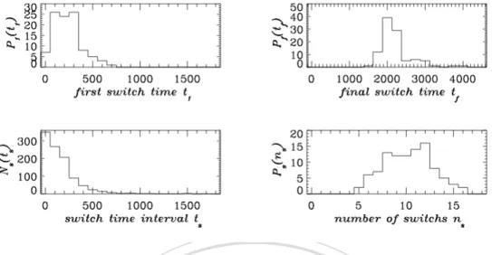
(43) Figure 2.3: statistical results of the switch times of strategies. 立. 政治大. Figure 2.3 summarizes statistical results of the switch times of strategies for all. ‧ 國. 學. agents in the sample society described in Table 2.2 and Fig. 2.2.. ‧. The asynchronous features lead to wide spreads in distributions for the numbers of players versus time of the first (upper left plot), the final (upper right plot). y. Nat. io. sit. switches of strategies, the statistics for the overall number of switches versus the. n. al. er. time interval in between consecutive switches (lower left plot) and that for the. Ch. i n U. v. number of player versus number of switches (lower right plot). The first switch of. engchi. strategy (upper left plot Fig. 2.3) can occur at time range from 100 steps (e.g. Fig. 2.2(c), agent no. 96) to 700 steps (e.g. Fig. 2.2(d), agent no. 17). The final switch before the strategies reaching convergence (upper right plot Fig. 2.3) can occur at time range from 1700 steps (e.g. Fig. 2.2(e), agent no. 48) to 4100 steps (e.g. Fig. 2.2(f), agent no. 5). The time interval (steps) between two consecutive switches (lower left plot Fig. 2.3) range from tens (e.g. Fig. 2.2(g), agent no. 1) to hundreds (e.g. Fig. 2.2(h), agent no. 14). The number of strategy switches for each agent (lower right plot Fig. 2.3) from 5 times (e.g. Fig. 2.2(i), agent no. 14) to 16 times (e.g. Fig. 2.2(j), agent no. 5). 25.

(44) In addition to considering models with various UD, we also introduce an intrinsic periodicity of activities for the society. Each period ends under the condition that the number of members of the society who have played the role as donor has reached MD since the end of last period. All strategy changes have to be made at the end of a period. Figure 2.4(a) summarizes the mechanism of the model by showing the flow chart of the simulation. In the social learning based updating procedure of strategy, we can also introduce the Metropolis algorithm to determine transition probability (Fig. (b)). In the work of this thesis, our simulations are carried out only for the cases of equivalence of zero temperature that is often used in a spin flipping (such as Potts. 政治大. model) simulation. The flow chart illustrates the strategy conversion process in detail.. 立. ‧. ‧ 國. 學. n. er. io. sit. y. Nat. al. Ch. engchi. 26. i n U. v.

(45) 立. 政治大. ‧ 國. 學 Fig. 2.4(a): Flow chart. ‧. Figures 2.4 (a) and (b) show the simulation process about the transactions in the. y. Nat. io. sit. Donor-Recipient game. We divided the process in two parts. The first stage is in Fig.. n. al. er. 2.4(a). We start the simulation in “transaction start”, then we randomly pick a pair of. Ch. i n U. v. agents, one as donor and the other as recipient. We set the parameters “player i” as. engchi. donor and “player j” as recipient. After each game step, the two parameters will updating inner items, the “player i” will updating both “wealth” and “reputation” while the “player j” will updating only “wealth”. The first stage simulation in the Donor-Recipient game has three conditions in order. The first condition is “number of players as donor = MD”, the second condition is “number of role as donor for player i = UD”, the third condition is “strategy adapted by player i subject to change”. The transactions only when the first condition and the second condition meet the standards, the game would go to the next stage.. 27.

(46) 立. 政治大. ‧ 國. 學 Fig. 2.4(b): Flow chart. ‧. In the Fig. 2.4(a), when the game transaction approaches to the step “ strategy. y. Nat. io. sit. adapted by player i subject to change ”, then go to the next flow chart Fig. 2.4(b). In. n. al. er. the Fig. 2.4(b), the transaction will enter to second stage. When the game transaction. Ch. i n U. v. approaches to the step “ Old strategy adapted by player i subject to change ”, the. engchi. player i will be given the quality to choose his new strategy in the next game step, otherwise, he has no choice and must keep the original strategy. Then the game transaction approaches to the step “ choosing: a candidate out of (q-1) strategies ”, the player could choose the candidate strategy out of his original strategy. After choosing the new strategy, the game transaction approaches to the step “ finding: accumulated income for old and for candidate over the whole society ”, and we set each agent an account for income calculation. Then the game transaction approaches to the step “ gain = − income flow for candidate + income flow for old ”, the gain could be. zero, positive or negative. The gain value will decide the next action, and then the 28.

(47) game transaction approaches to the branched step “Gain”. There are three branches in the decision. The diversity between the “gain=0” with the “gain<0” and the “gain>0” is that the “gain=0” will reset the “strategy adapted” selection by calling “random number r”. When “gain<0” or “gain=0, then random number r<0.5”, then “strategy adapted = candidate”, the new strategy is candidate strategy; When “gain>0” or “gain=0, then random number r≥0.5”, then “strategy adapted = old”, the new strategy is old strategy.. The calculation of “gain” is based on the difference ∆H between the income. 治政 decisions when the player needs to switch strategy. The大 spin-flipping algorithm used 立 in the simulation of Q-state Potts model is applied. In a “zero-temperature” flow H of the candidate strategy and that of the original strategy on making. ‧ 國. 學. equivalent simulation, there are three situations of the options as follows. When the. ‧. ∆H is less than zero, the agents will update his new strategy as the candidate strategy. On the contrary, when the ∆H is large than zero, the agents will update his new. y. Nat. er. io. sit. strategy as the old strategy. The last condition is that the ∆H is equal to zero, then we set the agent would rearrange his new strategy by calling a random number, and. n. al. Ch. i n U. v. the strategy updating decision would be made. If the random number is less than 0.5,. engchi. the updated strategy is the candidate strategy. On the other hand, if the random number is larger or equal to 0.5, the updated strategy is the old strategy.. 29.

(48) 治政 Fig. 2.5: Social learning theory大 illustration 立 ‧ 國. 學. The knowledge of H is obtained via a social learning procedure in simulation. Social learning theory is a perspective way the states that the social behavior is. ‧. learned primarily by observing and imitating the actions of others (Ormrod, J.E.. Nat. sit. y. (1999)). The social behavior is also influenced by being rewarded and/or punished for. n. al. er. io. these actions (Artino, A. R. (2007)). People learn through observing others’ behavior,. i n U. v. attitudes, and outcomes of those behaviors. “Most human behavior is learned. Ch. engchi. observationally through modeling: from observing others, one forms an idea of how new behaviors are performed, and on later occasions this coded information serves as a guide for action.” (Albert Bandura). Social learning theory explains human behavior in terms of continuous reciprocal interaction between cognitive, behavioral, and environmental influences. It talks about how both environmental and cognitive factors interact to influence human learning and behavior. It focuses on the learning that occurs within a social context. It considers that people learn from one another, including such concepts as observational learning, imitation, and modeling (Abbott, 2007). According to Bandura, 30.

(49) behavior can also influence both the environment and the person. It is the so-called “reciprocal causation”. Each of the three variables: environment, person, behavior influence each other. In the model society, the agents will update their strategy to improve their expected payoff through imitate other agents in the Donor-Recipient game. Agents randomly choose strategies and compare the difference ∆H in the income flow in payoffs during exogenously determined time intervals of steps (see Table 2.2 and Fig. 2.2). The strategy adjustments lead to new changes in wealth flow, the knowledge of. 治政 decision making in later-on strategy adjustments. 大立. which is collected as a new content of social learning and subsequently affects the. ‧ 國. 學. In the time evolution of donor-recipient games, the payoff of a strategy relies not only on the relative size of the offspring (the fraction) of each strategy, but also on the. ‧. fraction of individuals with a good reputation. Because the reputation of individuals is. sit. y. Nat. ever changing, it is hard to give a proper calculation of the payoff of a strategy. In. n. al. er. io. mean field analysis (Tongkui Yu et. al. 2011; Ohtsuki and Iwasa 2007), some. v. assumptions have made in order to overcome the hard calculations of the payoffs of. Ch. engchi. i n U. the strategies. In the agent-based model considered in our study, the asynchronous nature of the occurrence of events (see Fig. 2.2) renders such kind of analysis infeasible. It is found, nevertheless, the social-learning procedure strongly drive the evolution of our agent-based model society toward those attractors dominated by single strategies. We find as well that extended domains of attraction beyond isolated points are also possible.. 31.

(50) Chapter 3. Experimental Results Analysis In Chapter 3, we present the results of the agent-based simulation for Donor-Recipient game. We implement the rules of Donor-Recipient game simulation disclosed in Chapter 2. We use the characteristics of social learning mentioned in Section 2.3 to set the strategy’s switching rule in the donor-recipient game. The knowledge of social learning is realized separately in two forms, those collected either on a player-by-player basis or on that of event-by-event. Whenever the game runs accumulate to certain extent with MD members played the role of donor since last reset. 政治大. of counting and a donor happens to finish her personal role as donor for UD times, the. 立. donor will update her strategy according to the expected payoffs based on averages. ‧ 國. 學. calculated from accumulated records of wealth flows. The player based (or. ‧. “simple-averaged”) and the event based (or “weight-averaged”) calculations are performed, respectively, with all agents equally weighted and with all events equally. y. Nat. er. io. sit. weighted. The two ways correspond to situations of different information sufficiency.. al. v i n C h the donor can adjust each round of donor-recipient game, e n g c h i U her strategy as soon as she n. We consider two classes of simulations. One class has MD=1. That is, in finishing. has played the role of donor for UD times. We have carried out the simulations for a range of UD, which underscores the effect of frequency of strategy adjustment. It is found that the less frequent adjustment of frequency lead the society toward the common attractors close to the prediction of mean field analysis. We have focused on the cases with UD =2 in the simulations. The stable final states are quite different from the prediction of mean field analysis. Interestingly, a limit domain of attraction beyond isolated points is produced in the cases of strongly augmented norm with UD=2. 32.

(51) The second class has MD=50, which introduce a constraint on the number of members of the society to play the role of donor as a requirement for a donor just finishing a game to adjust her strategy, as soon as she herself alone has played the role of donor for UD times. In this study, we consider the cases with MD=1000 or 10000. The much less frequent strategy updating as compared with the first class renders the model societies behavior closer to the prediction of mean field analysis, in that the final stable states of time evolution are those isolated attractors dominated by single strategies. The latter are in agreement with the results of mean field analysis.. 立. 政治大. 3.1 Coarsened social learning versus refined social learning. ‧. ‧ 國. 學. n. er. io. sit. y. Nat. al. Ch. engchi. 33. i n U. v.

(52) The simulation outcome in simple social norm (GGBG): Using “simple-average” (player-weighted) in updating strategy. 立. 政治大. ‧ 國. 學. Figure 3.1(a): Population n in one typical experiment.. ‧. n. er. io. sit. y. Nat. al. Ch. engchi. i n U. v. Figure 3.1(b): Good reputation g of population in one typical experiment.. 34.

(53) The simulation outcome in simple social norm (GGBG): Using “simple-average” (player-weighted) in updating strategy. 立. 政治大. ‧ 國. 學. Figure 3.2(a): Population n in one typical experiment.. ‧. n. er. io. sit. y. Nat. al. Ch. engchi. i n U. v. Figure 3.2(b): Good reputation g of population in one typical experiment.. 35.

(54) We consider first the cases of MD=1 and UD=2. Figures 3.1 to Figure 3.4 are the time evolution for population in adapting each strategy and the corresponding “good” (G) reputed population, based on either of the two forms of knowledge in simulation of model society regulated by simple norm. In the social learning procedure, the competition between strategies can be determined based either on player-weighted or on event-weighted calculations. The cases of player-weighted (or simple-averaged) social learning are based on average over player number. All agents’ mean income flow will be weighted equally.. 治政 several rounds. To sum the average per agent in a single 大 round of changes in total 立 wealth, divided by the total number of society, will equal to per round to get the wealth Single strategy for each person with a single total change in wealth strategy involved. ‧ 國. 學. of a strategy change.. ‧. n. er. io. sit. y. Nat. al. C h H =score, engchi. i n U. v. Wi =wealth of agent i, N=population, fi =transaction number of agent i t =step. 36.