利用捲積類神經網路定位複雜背景中的條碼

(1)

國立臺灣大學生物資源暨農學院生物產業機電工程學系碩士論文

Department of Bio-Industrial Mechatronics Engineering College of Bioresources and Agriculture

National Taiwan University Master Thesis

利用捲積類神經網路定位複雜背景中的條碼 Barcode Localization Using Convolutional Neural

Networks

周子涵 Tzu-Han Chou

指導教授：郭彥甫博士 Advisor: Yan-Fu Kuo, Ph.D.

中華民國 104 年 7 月 July, 2015

(2)

i

ACKNOWLEDGEMENTS

I would like to express my sincere gratitude for assistance and support I received during my master project. First and foremost, I would like to express my sincerest gratitude to Professor Yan-Fu Kuo, my research advisor, for the continuous encouragement. I would like to thank Walter Ho for his suggestions in barcode extraction.

I would like to acknowledge the members of Lab 304, Walter, Tzu-Kuei, Wei-Tung, Cheng-Chun, Kai-Jyun, Andrew, Robert, Gado, Erica, and David who had accompanied me during my master thesis. I would especially thank Cheng-Liang again for the guidance on my research. I also want to express my appreciation for my friends, Jian-Jhih, Nian- ting, Jim, and Jacky with their friendships. Lastly but most importantly, I am deeply grateful to my family for their supporting.

(3)

ii

摘要

條碼長期被當作資訊的圖形辨識原件，不過在複雜背景中，可自動偵測出不同扭曲或傾斜的條碼，還是一大挑戰。此研究提出可自動偵測這些類型的條碼定位系統。在這研究中用來測試此系統的條碼，包含一維條碼 Code 39、Code 128 和 EAN- 13，與二維條碼 QR code。此定位系統利用捲積類神經網路(Convolutional neural network)演算法，辨別影像中條碼的區域。接著透過影像處理的方法，將區域中的條碼切取出來。實驗結果證實此條碼定位系統是可以偵測特定範圍的條碼大小，甚至對於模糊或變形的條碼也能有效的偵測能力。此演算法在 449 張實驗影像中，

可以達到 86.25%的偵測率與 78.55%切取率。

關鍵字：條碼定位，捲積類神經網路，影像處理，機器學習。

(4)

iii

ABSTRACT

Barcodes have been long used for data storage. Locating barcodes in images of complex background is an essential yet challenging step for automatic barcode reading.

This study aimed to detect and to extract one-dimensional Code 39, Code 128, and EAN- 13 barcodes and two-dimensional QR barcodes in images of arbitrary backgrounds. The proposed method involved a convolutional neural network for detecting parts of barcodes.

Once positive detection was confirmed, image processing algorithms were implemented to extract barcodes from the image. Experiments demonstrated that the proposed approach was able to locate barcodes of various module sizes and was robust to blurring, rotation, and deformation. The approach achieved an overall detection rate of 86.45% and an extraction rate of 78.55% using a set of 449 images.

Keywords: barcode localization, convolutional neural network, image processing, machine learning

(5)

iv

LIST OF TABLES

Table 3.1 Target module sizes for barcode detection. ... 11

(8)

vii

LIST OF FIGURES

Figure 3.1 Barcode localization system flow chart. ... 7

Figure 3.2 Training sample patches ... 9

Figure 3.3 CNN architecture. ... 10

Figure 3.4 Image pyramid for barcode localization ... 11

Figure 3.5 Scan line extraction process. ... 12

Figure 3.6 A demonstration of 1D barcode extraction operations ... 12

Figure 3.7 Area extraction for 2D barcodes. ... 14

Figure 3.8 An illustration of the inverse perspective transformation ... 14

Figure 3.9 A demonstration of 2D barcode extraction operations ... 14

Figure 4.1 Feature maps of the developed CNN. ... 16

Figure 4.2 Sample blurred patches for robustness analysis. ... 16

Figure 4.3 Detection rates on QR patches blurred using Gaussian smoothing. ... 17

Figure 4.4 Detection rates for barcodes of various module sizes ... 18

Figure 4.5 Detection rate of different module size in SP factors. ... 19

Figure 4.6 Processing time for detecting barcodes using the developed CNN. ... 20

Figure 4.7 Detection results of 1D barcodes. ... 21

Figure 4.8 Detection results of 2D QR barcodes. ... 21

Figure 4.9 Detection of shifted image. ... 22

(9)

viii

Figure 4.10 One-dimensional barcode extraction results. ... 23 Figure 4.11 Two-dimensional barcode extraction results. ... 23

(10)

1

CHAPTER 1. INTRODUCTION

1.1 Barcode

In the past few years, auto-robotics technologies have rapidly grown and robots are now seen all over factories replacing human labor. Robots play an important role in assisting tasks that average human beings cannot perform, especially in hazardous environments. In certain circumstances, robots require a machine vision system to provide information on their surrounding environments to perform and react properly.

The machine vision system should be able to recognize and describe objects. Each object may have an infinite number of different 2-D vision in respect to its position, posture, luminance and background. Barcodes are exceptional identification methods for labeling objects. They allow for the storage of high quantities of information as well as rapid and accurate identification at low cost.

Barcodes are symbols with encoded data that can be read by optical scanners.

Originally, one-dimensional (1D) barcodes consisted of a series of parallel lines with varying thickness and spaces. Because of limited storage capacity of the line-type patterns, barcodes later evolved into figures of two-dimensional (2D) forms such as rectangles and dots. These barcodes of 2D geometries, also referred to as 2D barcodes, were widely applied in various fields in recent years.

Barcode imaging for scanning differs from idea barcodes. Detection is based on feature characteristics of barcodes including the angle, distance, brightness, and resolutions of seized images which poses a large challenge. However, human’s visual ability can easily distinguish between barcode and other regions. In this study a simulation of the visual cortex method, convolutional neural networks (CNNs), was proposed to detect barcodes in an attempt to resolve this issue.

(11)

2

1.2 Convolutional neural networks

CNNs are multilayer perceptron classifiers. The network receives an input image and classifies the image into the labels that the model has trained. The pipeline of the system is divided into two sections, feature extraction and classification. The feature extraction consists of convolutions and subsampling operations inspired from visual cortexes. The architectural motivation is to achieve some degree of shift, scale, and distortion invariance in the extracted features. The operation extracts image features, which is called feature maps, at various scales based on the input image. The convolution layers detect local features using local receptive fields [1] in the input image. The weights are shared throughout the convolutional operation. Therefore, making the locations of the features become less important. Subsample layers performed data reduction and gained some scale invariance. In the classification, the neurons act like a classic fully connected multilayer perceptron network, which classify the features extracted from the previous section.

1.3 Objectives

In many previous research of barcode detection, the features were designed in idea conditions. The features may drastically vary in different environments and may lead to the results of greater misdetection. This work was aimed to detect partial 1D and 2D barcodes of arbitrary orientations and scales in complex backgrounds by using CNN. The targets to be detected were 1D barcodes, including Code 39, Code 128, and EAN-13, and 2D QR barcodes. The goals of this research were:

1. To collect a large training dataset of Code 39 and QR code images.

2. To identify if local patches of images are partial barcodes using CNN.

3. To extract barcode locations using image processing algorithms.

4. To evaluate the performance of the proposed model.

(12)

3

1.4 Organization

The remainder of this document was organized as follows. In Chapter 2, methods for detecting barcodes and convolution neural networks were reviewed. Chapter 3 presented an approach to automatically detecting barcodes in a complex background.

Results and discussion of this research were given in Chapter 4, and the conclusion of this work was giving in Chapter 5.

(13)

4

CHAPTER 2. LITERATURE REVIEW

2.1 One-dimensional barcode localization

The topic of automatic 1D barcode localization in images has been addressed by some literature. Zhang et al. [2] established approaches to detect non-uniformly illuminated and perspectively distorted 1D barcode based on the barcodes main orientation. Zamberletti et al. [3] proposed angle invariant 1D barcode detection algorithm. The algorithm applied multilayer perceptron network to detect 1D barcode by using the parameters of 2D Hough transform space. Some literature on local detection was also proposed. Wu et al. [4] proposed a method of dividing the image into horizontal strips. Then each horizontal strip was applied to determine whether it contained barcode or not. Lin et al. [5] presents a rotation-invariant algorithm for recognizing multiple 1D barcodes in an image. The maximum and minimum of 44 sub-image was derived from the input image. Next the difference of maximal and minimal image was applied to enhance the barcode region. Then a connected component analysis was conducted to segment the possible barcode regions. Chai et al. [6] investigated the recognition of EAN- 13 barcode. The methods divide the input image to patches and then examined each angle of connected components in a patch for recognition.

2.2 Two-dimensional barcode localization

In the tasks of 2D barcode detection, approaches have been proposed by some literature. Han et al. [7] suggested that wavelet analysis is effective to remove unevenly illumination with few loss of barcode information. Xu et al. [8] developed an approach for detecting blur 2D barcodes based on coded exposure algorithms. Ohbuchi et al. [9]

and Lin et al. [10] both applied the QR code finder patterns for detection. Leong et al.

[11] introduced the identification of the keypoints and lines of barcodes by using speeded

(14)

5

up robust features. Although these methods have high detection rates on certain barcodes, their performances may be affected by different image quality. Some of the methods reviewed above are based on handcrafted features using prior knowledge of specific conditions. For example, the ratio of black and white pixels may vary drastically when the barcode is tilted from the camera. Defining handcrafted features is labor-intensive and time consuming. In addition, inappropriate or insufficient handcrafted features may result in suboptimal detection rate.

2.3 Detecting barcodes using texture features

Humans are capable of detecting barcodes with arbitrary orientations and tilts in images of complex background. With only parts of a barcode, the texture parts can still be recognizable. Jain et al. [12] also commented that “The bar code region in an image can be considered as a homogeneous textured region which is distinct from other regions in the image.” Techniques like Gabor and wavelet filter have been developed for texture classification [13, 14]. Jain et al. [12] proposed an approach that localizes 1D barcode using Gabor filter for texture classification. Wang et al. [15] adapted the Gabor filter method with a neural network system to detect 2D barcodes.

2.4 Convolution neural network

CNNs has been reported by Tivive et al. [16] that the classifier outperforms other popular texture classification approaches. The network is not only robust on texture classification [16]. It is also very well known in image recognition. LeCun et al. [17-19]

proposed strategies of deep network design with back-propagation in recognition and proposed an architecture of CNN which became popular because of its outstanding performance in handwritten digit recognition. Then other CNN architectures were proposed for detecting faces [20, 21], identifying vehicle license plates [22], tracking

(15)

6

pedestrian movement [23], reading speed signs [24], and recognizing facial expression [25].

(16)

7

CHAPTER 3. MATERIAL AND METHODS

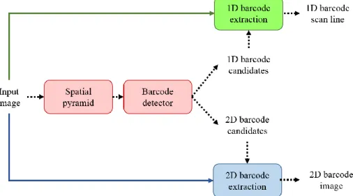
The proposed approach applied CNN classifiers to determine if local patches of an image are parts of barcodes. The detection process first involved a spatial pyramid that scaled the input images and then partitioned the scaled images into local patches. The local patches were subject to the CNN classifiers for barcode detection. Once positive detection for barcodes was confirmed, the local patches and their location information were then used for the subsequent barcode extraction. The flow chart of the barcode localization system is shown in Figure 3.1.

Figure 3.1 Barcode localization system flow chart.

3.1 Collection of training image patches

Image patches were collected for developing CNN classifier. First, 200 QR (version 7) and 200 Code 39 barcodes were created using an online generator. The barcodes contained dummy information. The Code 39 and QR barcodes were then printed using an electrophotographic printer (LaserJet M1132, HP; 600dpi) with densities of 13 and 15 mils per module, respectively. The printouts were scanned using a handheld barcode reader (9200 series, CipherLab; 752480 pixels), mimicking the typical process of

(17)

8

barcode scanning. For the QR barcodes, the printouts were placed approximately 10 and 20 cm away from the scanner. One hundred images were obtained with each distance setup. The distances were set to generate barcode images of approximately 7 and 4 pixels per module (ppm). For the Code 39 barcodes, 100 barcode images were obtained each at the distances of 5 cm and 10 cm away from the scanner. The distances were set to generate barcode images of approximately 7 and 3 ppm. The gathered code39 images were then artificially rotated to imitate variations of real world partial Code39 barcodes. The images were rotated counterclockwise with angles of 15, 30, 45, 60, 75, 90, 105, 120, 135, 150, and 165. A set of background images were also collected from various themes (e.g., posters, soda cans, and items). In summary, 500 image of Code 39 barcodes, 200 image of QR barcodes and 30 image of backgrounds were used as training data.

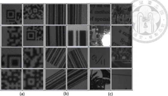
Training samples for the subsequent CNN classifier development were created from the collected images. The samples were patches of partial barcode images. In the process of sample patch creation, the images were downsampled by a factor of 0.5 in spatial resolution. The rescaled images were then segmented into 3232 patches in a non- overlapping manner. As a result, a total of 20,400 Code 39, 2,998 QR, and 8,745 background patches were gathered. Figure 3.2 illustrates some training sample patches.

(18)

9

Figure 3.2 Training sample patches of (a) 2D barcode, (b) 1D barcode and (c) background. The samples were patches of various module sizes and angles.

3.2 CNN architecture

A CNN system was developed for identifying partial barcode patches. The network was adapted from the architecture proposed by LeCun et al [19]. The input to the system was an image patch of 3232 pixels. The network determined if the patch was part of a 1D barcode, 2D barcode, or background. The CNN system consisted of six layers, including two convolutional layers C1 and C2, two subsampling layers S1 and S2, and two classification layers N1 and N2 (Fig. 3.3). Layers from C1 to S2 contained a series of planes, referred to as feature maps that functioned as trainable feature extractors. Layers C1 and C2, respectively, contained 6 feature maps of 28×28 pixels and 12 feature maps of 9×9 pixels. The feature maps were determined by convolution operations performed on a previous layer using trainable kernel matrices of 5×5 pixels. The convolution matrices were summed with a trainable bias and were fed into a sigmoid function to form a feature map. Therefore, layers C1 and C2, respectively, contained 156 (25×6+6) and 312 (25×12+12) trainable parameters. Layers S1 and S2, respectively, contained 6 feature

(19)

10

maps of 14×14 pixels and 12 feature maps of 5×5 pixels. These feature maps were the results of subsampling by a factor of 0.5 on the feature maps in layers C1 and C2.

Layers N1 and N2 formed a classical perception network to perform classification.

Layer N1 contained 300 neurons each of which connected to a pixel in layer S2. Layer N2

comprised 3 neurons fully connected to all the neurons in N1. The N2 neurons were outputs of a sigmoid function on the weighted sum of all the N1 neurons added biases.

Therefore, layers N1 and N2 contained 900 trainable weights and 3 trainable biases.

Figure 3.3 CNN architecture.

Stochastic back-propagation was applied to train the 1371 CNN parameters. The algorithm shuffled the training samples and arranged them into 478 batches .Each epoch go through every batch with back-propagation as input to update the model parameters.

The shuffle was performed at each epoch. The randomization of the training data was exploited to convergence at global minima. The system was trained by cycling through all the batches for 2000 epochs.

3.3 Detection of barcode with various module sizes

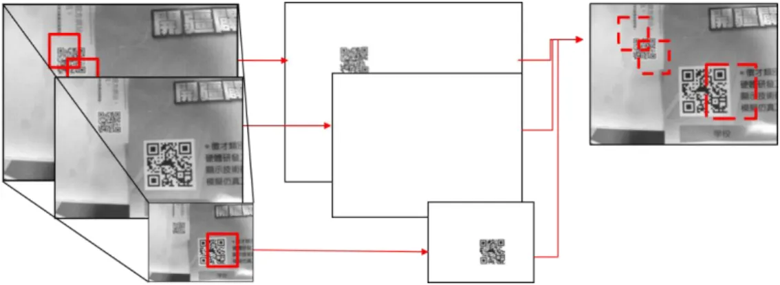
Spatial pyramid (SP) [21] was applied to enable the detection of barcodes at various scales. In the SP process, an input image was downsampled to various spatial resolutions, forming a pyramid of images (Fig. 3.4). The images were partitioned into patches of

(20)

11

32×32. The patches were then fed to the developed CNN classifier for detecting barcodes.

Once detected, the locations of the patches in the downsampled images were projected back to the input image. The regions, also referred to as blocks, corresponding to the inverse upsampling areas of the patches were identified for the subsequent process. In this study, the downsampling factors for the SP operation were set to 0.7, 0.5, and 0.3.

The factors were determined to detect barcodes of module sizes ranged between 2 and 11 ppm for 1D barcodes, and between 3 and 13 ppm for 2D barcodes (Table 3.1).

Figure 3.4 Image pyramid for barcode localization. The image pyramid on the left are the results of downsampling the original image by factor of 0.7, 0.5, and 0.3. The solid

frames represent the patches where barcode parts were detected. The dash frames are blocks of the detected barcode parts in the original image.

Table 3.1 Target module sizes for barcode detection.

Spatial pyramid factor 1D barcode (ppm) 2D barcode (ppm)

0.7 5 5.7

2.1 2.8

0.5 7 7

3 4

0.3 11 13.3

5 6.6

ppm: pixels per module

3.4 Scan line extraction for one-dimensional barcodes

The scan lines for 1D barcodes were extracted from the input image (Fig. 3.5). The extraction operation was modified from the technique proposed by Chai and Hock [8].

The approach first gathered the positive detection blocks obtained from the SP. Otsu

(21)

12

(a)

thresholding [26] and Canny edge detection [27] were performed to each block for enhancing the patterns of parallel lines of 1D barcodes. Hough transform [28] was next applied for identifying the orientations of the parallel lines in each block. The median orientation of the parallel lines for all the blocks was then determined. The scan lines were the lines passing through the centers of the blocks with a direction perpendicular to the median orientation. A demonstration of the 1D barcode extraction procedures are shown in Figure 3.6.

Figure 3.5 Scan line extraction process.

(d) (e) (f)

Figure 3.6 A demonstration of 1D barcode extraction operations: (a) input image (b) barcode candidates (c) block images (d) binarized block images (e) edge-detection

block images (f) extracted scan lines.

(b) (c)

(22)

13

3.5 Region extraction for two-dimensional barcodes

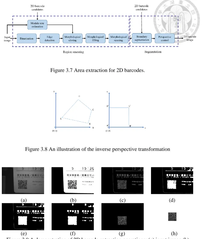
Complete regions of 2D barcodes were extracted from the input image (Fig. 3.7).

The extraction first involved a smearing of the regions that could potentially be barcodes.

Adaptive thresholding [29] and Canny edge detection were applied to determine the boundaries of the objects in the regions. The regions were then smeared using morphological closing and a square-shaped structuring element. The size of the structuring element was set to the barcode module size, which was estimated as the median pixel quantities of the black and white blobs between the centers of two consecutive positive detection patches in the image. The regions after smearing may still contain holes. Morphological filling was then applied to fill the holes. Morphological opening was next applied to reduce the noise sparkles in the background of the image.

The proposed smearing approach considered module sizes of the 2D barcodes. Therefore, it could precisely smear only the regions that were potentially to be barcodes and could separate background objects from the barcode regions.

The extraction subsequently involved segmentation and standardization. The smeared regions associated with positive detections from the CNN were identified.

Hough transforms were performed to detect the boundaries of the regions. Perspective transformation was next applied to restore the potentially distorted regions [30] to quadrangles (Figure 3.8). A demonstration of the 2D barcode extraction procedures are shown in Figure 3.9.

(23)

14

Figure 3.7 Area extraction for 2D barcodes.

Figure 3.8 An illustration of the inverse perspective transformation

(a) (b) (c) (d)

(e) (f) (g) (h) Figure 3.9 A demonstration of 2D barcode extraction operations: (a) input image (b) binarized image (c) edge-detection image (d) closed image (e) filled image (f) opened

image (g) barcode candidate image (h) output image.

(24)

15

CHAPTER 4. RESULTS AND DISCUSSION

In this chapter, the performance of the proposed barcode localization model was evaluated. First, the feature map of the trained CNN model was presented. Second, the sensitivity of the model was analyzed with variation of blurring, module size, and rotation using Code 39 and QR barcode as target detection. Next, detection speed of proposed method was illustrated. Then, the detection rate on the test image was discussed. Last, the extraction accuracy of test data, including the challenging conditions of tilted and incomplete barcodes were presented.

4.1 Feature maps of the trained CNN model

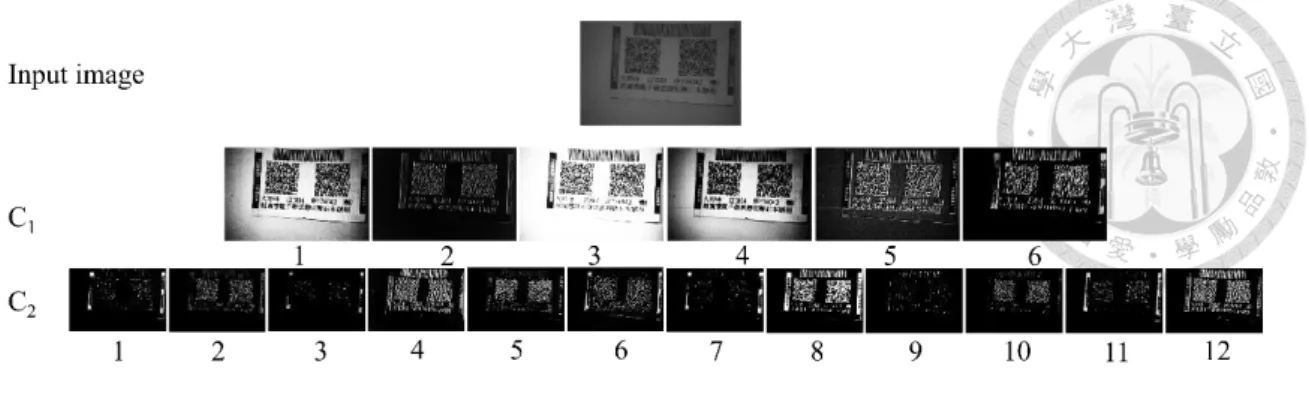
Figure 4.1 displays the feature maps of the developed CNN classifier for an input image. The maps were created by jointing the local feature maps of the input image patches in layers C1 and C2. The 6 C1 feature maps demonstrate contrast enhancement, edge detection, and complements of the input image. These operations improve the localization of barcodes because barcode areas are usually of high contrasts and distinct texture features. The non-uniform illumination is alleviated in C2, such that the dark corners in C1-1 and C1-4 are removed in C2 feature maps. Some C2 feature maps exhibit resemblances of barcode regions. For example, the feature map C2-3 feature map shows high relatively density gray levels in the regions corresponding to the 2D barcodes in the input image. The feature map C2-7 extracts the background objects. One-dimensional barcode regions can be identified by combining the features of C2-6 and C2-8.

(25)

16

Figure 4.1 Feature maps of the developed CNN.

4.2 Robustness of the CNN classifier to blur, module size variation, and rotation

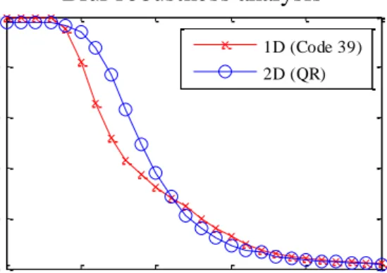
The robustness of the CNN to blur was investigated. In the analysis, additional 1,423 and 2,560 patches of Code39 and QR barcodes, respectively, were collected. These patches were correctly identified as barcode patches using the developed CNN. The patches were blurred using a Gaussian smoothing filter [31] with a 3×3 mask and standard deviations (SD) ranged from 0 to 2.5 (Fig. 4.2). The blurred patches were then fed to the CNN for testing.

Figure 4.2 Sample blurred patches for robustness analysis.

(26)

17

Figure 4.3 displays the detection rates on the patches blurred of various SD. The detection rate remained reasonably high (98%) when the SD was 0.5. The rate drops abruptly when the SD varied from 0.5 to 1.5. The rates were still over 50% even with a SD of 1.

Figure 4.3 Detection rates on QR patches blurred using Gaussian smoothing.

The detection rates for barcodes of various module sizes were investigated. In the analysis, additional 20 test images of Code 39 and QR barcodes for each set of module size, respectively, were acquired. The distance between the barcode printouts and reader was appropriately adjusted, so that the module sizes of the images were approximately 3, 5, 7, and 9 ppms. Efforts were made to avoid rotation or tilt during the image acquisition.

The acquired images were next clipped into patches to test the detection rates of various SP factors.

For the Code 39 patches (Fig. 4.4a), the CNN achieved detection rates higher than 70% for almost all the module sizes using all the SP factors. The only exception was the combination of the module size 9 ppm and the SP factor 0.7. This is because the SP factor of 0.7 was destined to detect barcodes of smaller module sizes. The maximum detection rates for barcodes of module sizes 3, 5, 7, and 9 ppms were 100%, 99.93%, 99.07%, and

0 0.5 1 1.5 2 2.5

0 20 40 60 80 100

Standard deviation of Gaussian smoothing

Accuracy (%)

Blur robustness analysis

1D (Code 39) 2D (QR)

(27)

18

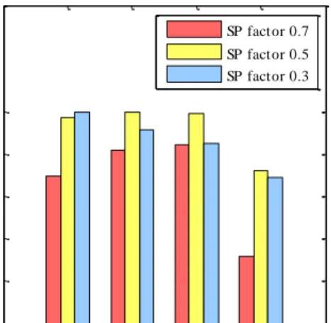
71.96%, respectively. For the QR patches (Fig. 4.4b), the CNN achieved detection rates higher than 90% for all the module sizes using various SP factors. In general, the CNN could more accurately recognize barcodes of larger module sizes using smaller SP factors, and vice versa. This observation indicates that using various SP factors improves the detection of QR barcodes of various module sizes. The maximum detection rates for barcodes of module sizes 3, 5, 7, and 9 ppms were 88.07%, 89.21%, 83.31%, and 99.83%, respectively.

(a)

(b)

Figure 4.4 Detection rates for barcodes of various module sizes for (a) 1D Code 39 and (b) 2D QR.

3 5 7 9

0 20 40 60 80 100

Pixels per module

Accuracy (%)

Code 39 barcode SP factor analysis

SP factor 0.7 SP factor 0.5 SP factor 0.3

3 5 7 9

0 20 40 60 80 100

Pixels per module

Accuracy (%)

QR barcode SP factor analysis

SP factor 0.7 SP factor 0.5 SP factor 0.3

(28)

19

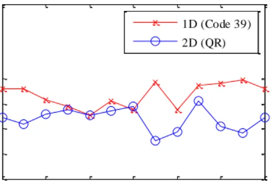
The sensitivities of the CNN for detecting barcodes of various rotational angles were examined. In the analysis, an additional 200 test images of Code 39 and QR barcodes, respectively, were collected. The distance between the barcode printouts and reader was 10cm. The test images were then downsampled to 0.5 and were then artificially rotated from -90 to 90 with an increment of 15. The patches of the rotated barcodes were gathered. Figure 4.5 illustrates the average detection rates of the patches. The mean detection rates for the Code 39 and QR barcodes reached 93.46% and 83.91%, respectively. The detection rates for the Code 39 barcode patches at some angles were not optimal. However, a barcode usually comprises multiple patches. The cumulative detection probability for a barcode composed of multiple patches could be reasonably high.

Figure 4.5 Detection rate of different module size in SP factors.

4.3 The process time of the proposed barcode detection

The process time of the proposed barcode detection system was presented. The process involved image pyramid construction and CNN classification. Figure 4.6 shows the average processing time of 449 images (480752 pixels) at each stage of detection.

In each image, the patches of SP factor 0.7, 0.5, and 0.3 were 160, 77, and 28, respectively.

-90 -60 -30 0 30 60 90

60 70 80 90 100

Rotation angle (degrees)

Accuracy (%)

Barcode rotation sensitivity analysis

1D (Code 39) 2D (QR)

(29)

20

The time for SP factor 0.7 was 0.1063 seconds. It takes up about 54.42% of the total process. This results shows the processing time is proportion to the number of patches.

The barcode detection was performed using a personal computer with a CPU of 3.4 GHz Intel i5. On average, the total process time of the detection is approximately 0.1953 seconds per frame (5FPS).

Figure 4.6 Processing time for detecting barcodes using the developed CNN.

4.4 The results of barcode detection on the test data

The proposed barcode detection system was evaluated using a set of 491 images.

The images were collected from the internet or photographed by the authors. The images were not selected based on any specific criterion and consisted of a large collection of barcodes with various module size, rotation, tilt, and contrast. Most of the images have complex backgrounds. Each image contains one or more 1D and/or 2D barcodes. A total of 300 1D barcodes (including Code 39, Code 128, and EAN-13) and 300 2D QR

0 0.025 0.05 0.075 0.1

Processing time (s)

Barcode detection proscessing time

Image pyramid SP factor 0.7 SP factor 0.5 SP factor 0.3

(30)

21

barcodes were collected. The developed CNN achieved detection rates of 88.33% and 77.33% for 1D and 2D barcodes, respectively. Figures 4.7 and 4.8 demonstrates some detection results of 1D and 2D barcodes, respectively.

Figure 4.7 Detection results of 1D barcodes. The CNN developed CNN classifier is capable of detecting 1D (a) Ean-13, (b) Code 128, (c) Ean-13, (d) Code 39, (e) Code 39,

(f) Code 128, (g) Ean-13, and (h) Ean-13.

Figure 4.8 Detection results of 2D QR barcodes. The developed CNN classifier is capable of detecting (a) double barcodes, (b) a barcode with small module size, (c) a tilted barcode, (d) typical barcode, (e) a barcode in complex background, (f) different barcode version, (g) double incomplete barcode (h) incomplete barcode with different

version.

The false negative detection of 2D barcodes were investigated. In the analysis, the images of false negative detection were artificially shifted to the right by some pixels, mimicking the process of aiming adjustment during a barcode scanning (Fig. 4.9). The shifts did not affect the completeness of the barcodes. With the shifts, 19 of the 68 false

(31)

22

negative barcodes could be detected. The detection rate of 2D barcode increase to 83.66%.

Since the CNN performed the detection at a rate of 5 FPS, the detection rate of 2D barcodes could be improved with real-time continuous scanning.

Figure 4.9 Detection of shifted image. The red arrows in the images illustrate the original images shifted right by x pixels.

4.5 The results of barcode extraction on the test data

Figure 4.9 Detection of shifted image. The red arrows in the images illustrate the original images shifted right by x pixels. The images with positive barcode detection were subsequently used for evaluating the performance of the proposed barcode extraction.

The image contained 265 1D and 232 2D barcodes Forty-three 2D barcodes in the image set were incomplete (Fig.4.8 (g) and Fig.4.8 (h)). These incomplete barcodes could be detected but could not be extracted. After excluding the incomplete samples, the extraction rates achieved 89.43% and 67.67% for the 1D and 2D barcodes, respectively.

Figure 4.10 and Figure 4.11 display the results of 1D and 2D barcode extraction. The capability of partial barcode detection is essential, especially for eyes-free barcode detection applications.

(32)

23

Figure 4.10 One-dimensional barcode extraction results.

Figure 4.11 Two-dimensional barcode extraction results.

(33)

24

CHAPTER 5. CONCLUSION

This study presented a framework for locating 1D and 2D barcodes in image of complex background. The approach identified partial barcode patches of various module sizes using a CNN and an SP scheme. The detected patches of the same barcode were then connected and extracted from the background for decoding. This strategy of partial barcode patch detection made it possible to identify barcode with large degrees of distortion. Analysis demonstrated that the proposed approach was robust to blur, and rotation of barcode images. The proposed approach reached a detection rate of 88.83%

and 83.66% and extraction rate of 89.43% and 67.67% for 1D and 2D barcode from the test dataset.

(34)

25

REFERENCES

1. Hubel, D.H. and T.N. Wiesel, Receptive fields, binocular interaction and functional architecture in the cat's visual cortex. The Journal of physiology, 1962. 160(1): p.

106.

2. Chunhui, Z., et al. Automatic Real-Time Barcode Localization in Complex Scenes.

in IEEE International Conference on Image Processing. 2006. p. 497-500.

3. Zamberletti, A., I. Gallo, and S. Albertini. Robust Angle Invariant 1D Barcode Detection. in IAPR Asian Conference on Pattern Recognition. 2013. p. 160-164.

4. Wu, X.-S., L.-Z. Qiao, and J. Deng. A New Method for Bar Code Localization and Recognition. in International Congress on Image and Signal Processing. 2009. p. 1- 6.

5. Lin, D.-T., M.-C. Lin, and K.-Y. Huang, Real-time automatic recognition of omnidirectional multiple barcodes and DSP implementation. Machine Vision and Applications, 2011. 22(2): p. 409-419.

6. Chai, D. and F. Hock. Locating and Decoding EAN-13 Barcodes from Images Captured by Digital Cameras. in International Conference on Information Communications and Signal Processing. 2005. p. 1595-1599.

7. Dong, H., et al. 2D barcode image binarization based on wavelet analysis and Otsu's method. in International Conference on Computer Application and System Modeling. 2010. Taiyuan: IEEE. p. 30-33.

(35)

26

8. Wei, X. and S. McCloskey. 2D Barcode localization and motion deblurring using a flutter shutter camera. in IEEE Workshop on Applications of Computer Vision.

2011. p. 159-165.

9. Ohbuchi, E., H. Hanaizumi, and L.A. Hock. Barcode readers using the camera device in mobile phones. in International Conference on Cyberworlds. 2004. p. 260- 265.

10. Lin, J.-A. and C.-S. Fuh, 2D Barcode Image Decoding. Mathematical Problems in Engineering, 2013. 2013: p. 10.

11. Leong, L.K. and W. Yue, Extraction of 2D barcode using keypoint selection and line detection, in Advances in Multimedia Information Processing. 2009, Springer.

p. 826-835.

12. Jain, A.K. and Y. Chen. Bar code localization using texture analysis. in Proceedings of the Second International Conference on Document Analysis and Recognition.

1993. p. 41-44.

13. Jain, A.K. and F. Farrokhnia. Unsupervised texture segmentation using Gabor filters. in IEEE International Conference on Systems, Man, and Cybernetics. 1990.

p. 14-19.

14. Arivazhagan, S., L. Ganesan, and S.P. Priyal, Texture classification using Gabor wavelets based rotation invariant features. Pattern Recognition Letters, 2006.

27(16): p. 1976-1982.

(36)

27

15. Wang, M., L.-N. Li, and Z.-X. Yang. Gabor filtering-based scale and rotation invariance feature for 2D barcode region detection. in International Conference on Computer Application and System Modeling. 2010. IEEE. p. V5-34-V5-37.

16. Tivive, F.H.C. and A. Bouzerdoum. Texture Classification using Convolutional Neural Networks. in IEEE Region 10 Conference. 2006. p. 1-4.

17. LeCun, Y., Generalization and network design strategies. Connections in Perspective. North-Holland, Amsterdam, 1989: p. 143-55.

18. Le Cun, B.B., et al. Handwritten digit recognition with a back-propagation network.

in Advances in neural information processing systems. 1990. Citeseer.

19. LeCun, Y., et al., Gradient-based learning applied to document recognition.

Proceedings of the IEEE, 1998. 86(11): p. 2278-2324.

20. Lawrence, S., et al., Face recognition: A convolutional neural-network approach.

IEEE Transactions on Neural Networks, 1997. 8(1): p. 98-113.

21. Garcia, C. and M. Delakis, Convolutional face finder: A neural architecture for fast and robust face detection. IEEE Transactions on Pattern Analysis and Machine Intelligence, 2004. 26(11): p. 1408-1423.

22. Chen, Y.-N., et al. The application of a convolution neural network on face and license plate detection. in International Conference on Pattern Recognition. 2006.

IEEE. p. 552-555.

23. Szarvas, M., U. Sakai, and J. Ogata. Real-time pedestrian detection using LIDAR and convolutional neural networks. in IEEE Intelligent Vehicles Symposium. 2006.

IEEE. p. 213-218.

(37)

28

24. Peemen, M., B. Mesman, and C. Corporaal. Speed sign detection and recognition by convolutional neural networks. in Proceedings of the 8th International Automotive Congress. 2011. p. 162-170.

25. Simard, P.Y., D. Steinkraus, and J.C. Platt. Best practices for convolutional neural networks applied to visual document analysis. in International Conference on Document Analysis and Recognition. 2003. IEEE Computer Society. p. 958-958.

26. Otsu, N., A Threshold Selection Method from Gray-Level Histograms. IEEE Transactions on Systems, Man and Cybernetics, 1979. 9(1): p. 62-66.

27. Canny, J., A Computational Approach to Edge Detection. IEEE Transactions on Pattern Analysis and Machine Intelligence, 1986. PAMI-8(6): p. 679-698.

28. Duda, R.O. and P.E. Hart, Use of the Hough transformation to detect lines and curves in pictures. Commun. ACM, 1972. 15(1): p. 11-15.

29. Bradley, D. and G. Roth, Adaptive Thresholding using the Integral Image. Journal of Graphics, GPU, and Game Tools, 2007. 12(2): p. 13-21.

30. Ohbuchi, E., H. Hanaizumi, and L.A. Hock. Barcode readers using the camera device in mobile phones. in Cyberworlds, 2004 International Conference on. 2004.

p. 260-265.

31. Gonzalez, R.C. and R.E. Woods, Digital Image Processing (3rd Edition). 2006:

Prentice-Hall, Inc.