Based Functions

Chapter 3

Learning Algorithms for RBF Functions and Subspace

Based Functions

Lei Xu

Chinese University of Hong Kong and Beijing University, PR China

BACKGROUND

The renaissance of neural network and then machine learning since the 1980’s is featured by two streams of extensive studies, one on multilayer perceptron and the other on radial basis function networks or shortly RBF net. While a multilayer perceptron partitions data space by hyperplanes and then making subsequent processing via nonlinear transform, a RBF net partitions data space into modular regions via local structures, called radial or non-radial basis functions. After extensive studies on multilayer perceptron, studies have been turned to RBF net since the late 1980’s and the early 1990’s, with a wide range applications (Kardirkamanathan, Niranjan, & Fallside, 1991; Chang & Yang, 1997; Lee, 1999;

ABSTRACT

Among extensive studies on radial basis function (RBF), one stream consists of those on normalized RBF (NRBF) and extensions. Within a probability theoretic framework, NRBF networks relates to nonpara- metric studies for decades in the statistics literature, and then proceeds in the machine learning studies with further advances not only to mixture-of-experts and alternatives but also to subspace based functions (SBF) and temporal extensions. These studies are linked to theoretical results adopted from studies of nonparametric statistics, and further to a general statistical learning framework called Bayesian Ying Yang harmony learning, with a unified perspective that summarizes maximum likelihood (ML) learning with the EM algorithm, RPCL learning, and BYY learning with automatic model selection, as well as their extensions for temporal modeling. This chapter outlines these advances, with a unified elaboration of their corresponding algorithms, and a discussion on possible trends.

by Olivas, Guerrero, Sober, Benedito, & Lopez, IGI Global publication, pp60-94.

Mai-Duy & Tran-Cong, 2001; Er, 2002; Reddy & Ganguli, 2003; Lin & Chen 2004; Isaksson, Wisell,

& Ronnow, 2005; Sarimveis, Doganis, & Alexandridis, 2006; Guerra & Coelho, 2008; Karami & Mo- hammadi, 2008).

In the literature of machine learning, advances on RBF net can be roughly divided into two streams.

One stems from the literature of mathematics on multivariate function interpolation and spline approxi- mation, as well as Tikhonov type regularization for ill-posed problems, which were brought to neural networks learning by (Powell, 1987; Broomhead & Lowe, 1998; Poggio & Girosi, 1990; Yuille &

Grzywacz, 1989) and others. Actually, it is shown that RBF net can be naturally derived from Tikhonov regularization theory, i.e. least square fitting subjected to a rotational and translational constraint term by a different stabilizing operator (Poggio & Girosi, 1990; Yuille & Grzywacz, 1989). Moreover, RBF net has also been shown to have not only the universal approximation ability possessed by multilayer perceptron (Hartman, 1989; Park & Sandberg,1993), but also the best approximation ability (Poggio &

Girosi, 1990) and a good generalization property (Botros & Atkeson, 1991).

The other stream can be traced back to Parzen Window estimator proposed in the early 1960’s. Stud- ies of this stream progress via active interactions between the literature of statistics and the literature of machine learning. During 1970’s-80’s, Parzen window has been widely used for estimating probability density, especially for estimating the class densities that are used for Bayesian decision based classification in the literature of pattern recognition. Also, it has been introduced into the literature of neural networks under the name of probabilistic neural net (Specht, 1990). By that time, it has not yet been related to RBF net since it does not directly relates to the above discussed function approximation purpose.

In the literature of neural networks and machine learning, Moody & Darken (1989) made a popular work via Gaussian bases as follows:

f x w_{j j} x c_{j j} x c e

j k

j j j

x c_j^T _j x

( )= ( - , ), ( - , )= ^{. ( ) (}

=

- - -

å

^{j S j S S-}

1

0 5 ¹

^ccj)

å

^k_j=1e^{-0 5. (x c-j)T -j (x c-j)}.

S1

(1) This normalized type of RBF net is featured by

j_{j j j}

j k

x c

( - , )=

å

= ^S 1

1, (2)

and thus usually called Normalized RBF (RBF). Moody & Darken (1989) actually considered a special case S_j = s_j²I . Unknowns are learned from a set of samples via a two stage implementation. First, a clustering algorithm (e.g., k-means) is used to estimate c_i as each cluster’s center. Second, j_j( )x is calculated for every sample and unknowns w_j are estimated by a least square linear fitting. Nowlan (1990) proceeded along this line with Σ_j considered in its general form such that not only the receptive field of each base function can be elliptic instead of radial symmetrical, but also the well known EM algorithms (Redner & Walker, 1984) are adopted for estimating c_i and Σ_j with better performances than that by a clustering algorithm.

In the nonparametric statistics literature, extensive studies have also been made towards regression tasks under the name of kernel regression estimator, which is an extension of Parzen window estima- tor from density estimation to statistical regression (Devroye, 1981&87). In (Xu, Krzyzak, & Yuille,

1992&94), kernel regression estimators are shown to be special cases of NRBF net. In help of this connection, theoretical results available on kernel regression have been adopted, which cast new lights on the theoretical analysis of NRBF net in several aspects, e.g., universal approximation extended to statistical consistency, convergence extended to convergence rate, etc.

Another line of studies in the early 1990 is featured by using the mixtures-of-experts (ME) (Jacobs, Jordan, Nowlan, & Hinton, 1991) for regression:

f x g x_j f x_{j j}

j

( )= k ( , ) ( , ),

å

= ^{f q} 1

(3)

where each g x_j( , )φ is a function implemented by a three layer forward networks, and 0£g x_j( , )f £1 is called gating net. This f x g x_j f x_{j j}

j k

( )= ( , ) ( , )

å

= ^{f q} 1

is actually a regression equation of a mixture of conditional distribution as follows:

q(z x g x_j q(z x j f x E z f x

j k

q z x j

| )= ( , ) | , ) ( )= _{( | )} (

å

= ^f 1

, with and ,, )q_j =E_{q z x j( | , )}z.

(4) One typical example is q z x j( | , )=G z f x( | ( , ),_j q G_{j j}), where G u( | , )m S denotes a Gaussian den- sity with mean vector μ and covariance matrix Σ. All the unknowns in this mixture are estimated via the maximum likelihood (ML) learning by a generalized EM algorithm (Jordan & Jacobs, 1994; Jordan &

Xu, 1995).

Furthermore, a connection has been built between this ME model and NRBF net such that the EM algorithm has been adopted for estimating jointly all the parameters in a NRBF net to improve subop- timal performances due to a two stage implementation. In sequel, we start at this EM algorithm, and then introduce further advances on NRBF studies. Not only basis functions is extended from radial to subspace based functions, and further to temporal modeling, but also studies further proceed to tackle model selection problem, i.e., how to determine the number k and the subspace dimensions.

THE EM ALGORITHM AND BEYOND: ALTERNATIVE ME VERSUS ENRBF

Xu, Jordan & Hinton (1994&95) proposed an alternative mixtures-of-experts (AME) via a different gat- ing net. Considering each expert G z f x( | ( , ),_j q G_{j j}) supported on a Gaussian G x( | ,m S_{j j}) or generally an expert q z x( | ,q_j) supported on a corresponding q x( | )f_j , we have that p z x( | ) is supported on a finite mixture q x( | )f with its corresponding posteriori as the gating net:

q(z x g x q z x g x q x

j j q x

j k

j

j j

| ) ( , ) ( | , ), ( , ) ( | ) ( | ) ,

= =

å

= ^{f q f a} _f^f 1

q x _jq x _j , 0

j k

j j

j k

( | )f = a ( | )f £a, a = .

= =

å å

1 1

1

(5)

Given a training set { , }z x_{t t t}^N₌₁, parameter learning is made by the ML learning on the joint distribu- tion q(z x q x| ) ( | )f =

å

^k_j=1a_jq x( | ) ( | , )f_j q z x q_j , which is implemented by the EM algorithm, i.e., Algorithm 1(a). Details are referred to (Xu, Jordan & Hinton, 1995).

We observe that the M step decouples the updating in parts. The one for updating θ_j of each expert is basically same as in (Jacobs, Jordan, Nowlan, & Hinton, 1991) except here we get a different p(j | z_t, x_t) as the E step. The ones for updating the unknowns a f_j, _j of the gate can be made via letting p(j | z_t, x_t) to take the role of p(j | x_t) in the M step of the EM algorithm on a finite mixture or Gaussian mixture (Redner & Walker, 1984; Nowlan, 1990).

Alternatively, we can use the resulted p(j | z_t, x_t) to replace g x_j( , )f as the gate in eqn.(5), i.e., q z x( | )_{t t} =

å

^k₌₁p(^| , ) ( | , ) .z x q z x_{t t t t} q^ (6a)

When z_t is discrete, this equation is still directly computable on testing samples. However, when z_t takes real values that are usually not available on testing samples, we can not directly use p(j | z_t, x_t) to Figure 1. Algorithm 1: EM algorithm for alternative mixture of experts and NRBF nets

replace g x_j( , )f as the gate in eqn.(4). Instead, we get an estimate f x_j( , )_t q =_j E_{q z x j( | , )}z as zˆ_t, from which we usually have either q z x(ˆ | , )_{t t} q_j in a constant or q z x(ˆ | , )_{t t} q_j =j q( )_j , e.g., j q( )_j =( )2p ^{-0 5.d} |G_j|^{-0 5.} for q z x( | , )q_j =G z f x( | ( , ),_j q_j G_j). Thus, we get

p(j x z q x q z x q x q z x

j j j

j j j

j

| , ) k ( | ) ( | , ) ( | ) ( | , ),

=

å

=

a f q

a f q

1

for aan integer z,

p(j x z q x

t q x

j j j

j j j

j

| , ˆ ) k ( | ) ( ) ( | ) ( )

=

å

=

a f j q a f j q

1

,, for a real z.

(6b)

which takes the place of g x_j( , )f as the gate in eqn.(4).

Furthermore, NRBF net is obtained as a special case, as shown in Algorithm I(b). In this case, the regression function in eqn. (3) becomes

f x f x_{j j j} x c_{j j}

j k

( )= ( , ) ( - , ),

å

= ^{q j S} 1

(7)

which is actually an extension of NRBF net with a constant w_j generalized to a general regression f x_j( , )q_j . That is, we are lead back to eqn.(2) when f x_j( , )q =_j w_j and the so called Extended NRBF (ENRBF) net (Xu, Jordan & Hinton, 1994&95; Xu, 1998) when f x_j( ,θ =_j) W x_j +w_j. Straightforwardly, we can use the EM algorithm in Algorithm I to update all the unknowns, from which we can also obtain differ- ent versions of the EM algorithms at various particular cases (Xu, 1998). For an example, it improves the two stage implementation of learning NRBF by (Nowlan, 1990) in a sense that the updating of c_i, Σ_j also takes w_j in consideration via p(j | z_t, x_t), while the updating of w_j takes c_i and Σ_j in consideration via this p(j | z_t, x_t) too.

It is interesting to further elaborate the connection between RBF net and the ME models from a dual perspective. For the RBF net by eqn.(2), we seek a combination of a series of basis functions j_j(x-c_j,S_j) via linear weights of w_j. For the ME model by eqn.(3), we seek a convex combination of a series of functions f x_j( , )q_j weighted by g x_j( , )f that actually takes the role of the basis function j_j(x-c_j,S_j) in eqn.(2). That is, there is a dual perspective that can swap the roles of the weighting coefficients and what are weighted. The ME perspective provides extensions of RBF net from classical radial basis functions j_j(x-c_j,S_j) to g x_j( , )f =a_jG x( | ,m_j ^S_j)

å

^k_{j 1=} a_jG x( | ,m_j ^S_j) and further to p(j | z_t, x_t) in eqn.(6a) and eqn.(6b). Moreover, in addition to NRBF net with f x_j( , )q =_j w_j and ENRBF net with f x_j( ,θ =_j) W x_j +w_j, f x_j( , )q_j can also be implemented by a multilayer networks (Jacobs, Jordan, Nowlan, & Hinton, 1991), which actually combines the features of both NRBF net and three layer forward networks.

TWO STAGE IMPLEMENTATION VERSUS AUTOMATIC MODEL SELECTION Using a structure by a RBF net or a ME model to accommodate a mapping x → z, one needs a learn- ing algorithm that estimates unknown parameters in this structure. The performance of a resulted RBF or ME can be measured via a set of testing samples by either a square error z_t - ( )f x_t ² for function approximation or classification error for pattern recognition, as well as the likelihood ln p(z_t | x_t) for distribution approximation. Correspondingly, an algorithm is guided by one of these purposes via a set of training set. The classic RBF net studies considers minimizing the square error z_t - ( )f x_t ² on a set X_N ={ }x_{t t}^N₌₁ of training samples. The studies (Jacobs, Jordan, Nowlan, & Hinton, 1991; Jordan

& Jacobs, 1995) on the ME model considers maximizing the likelihood ln p(z_t | x_t) on X_N, while the alternative ME considers maximizing the likelihood ln p(z_t, x_t) on X_N (Xu, Jordan & Hinton, 1994&95).

However, a good performance on a training set is not necessarily good on a testing set, especially when the training set consists of a small size of samples. The reason is too many free parameters to be deter- mined. Studies towards this problem have been widely studied along two directions in the literature of statistics and machine learning.

One is called regularization that adds some constraint or regularity to the unknown parameters, the selected structure, and the training samples (Powell, 1987; Poggio, & Girosi, 1990). Readers are referred to (Xu, 2007c) for a summary of typical regularization techniques studied in the literature of learning. One example is smoothing X_N by a Gaussian kernel with a zero mean and a unknown smoothing parameter h as its variance, i.e., instead of directly using X_N for training we consider p( |X X_N, )h =G(X X- _N | ,0h I² ). Actually, maximizing ln p(z_t, x_t) by the alternative ME can be regarded as maximizing ln ( | )p z x_{t t} plus a term ln ( | )q x f that adds certain constrain on samples of x_t. This is an example of a family of typical regularization techniques, featured by the format ln p(z_t | x_t) or ln ( | )p z x_{t t} + l qW( , , )z x_{t t} , where

W( )q or W( , , )q z x_{t t} is usually called stabilizer or regularizor, and λ is called regularization strength.

However, we encounter two difficulties to impose a regularization. One is the difficulty of appro- priately controlling a regularization strength λ, which is usually able to be roughly estimated only for a rather simple structure via either handling the integral of marginal density or in help of cross validation (Stone, 1978), but with very extensive computing costs. The other is the difficulty of choosing an ap- propriate W( )q or W( , )q x_t based on a priori knowledge that we are usually not available and difficult to get. Instead, an isotropic or nonspecific stabilizer is usually imposed, e.g.,. W( )q = q². This type of isotropic or nonspecific regularization faces a dilemma. We need a regularization on a structure S_k(Q_k) with extra parts, while an isotropic or nonspecific regularization can not discard the extra parts but still let them in action to blur those useful parts. For an example, given a set of samples { , }z x_{t t} that come from a curve z = x² + 3x + 2, if we use a polynomial z =

å

_i^k₌0a x_i ⁱof an order k > 2 to fit the data set, we desire to force all the parameters {a_i, i ≥ 3} to be zero, while minimizing q ² =

å

i₌₀^ai2

k fails to treat the parameters {a_i, i ≥ 3} differently from the parameters {a_i, i ≤ 2}.

To tackle the problems, we turn to consider the other direction that consists of those efforts made under the name of model selection. It refers to select an appropriate one among a family of infinite many candidate structures { (S_k Q_k)} with each S_k(Q_k) in a same configuration but in different scales, each of which is labeled by a scale parameter k in term of one integer or a set of integers. Selecting an

appropriate k means getting a structure that consists of an appropriate number of free parameters. For a structure by a RBF net or a ME model, this k is simply the number k of bases or experts. Usually, a maximum likelihood (ML) principle based learning is not good for model selection. The EM algorithm in Algorithm I works well with a pre-specified number k of bases or experts. The performance will be affected by whether an appropriate k is selected, while how to determine k is a critical problem.

Many efforts have been made towards model selection for over three decades in past. The classical one is making a two stage implementation. First, enumerate a candidate set K of k and estimate the unknown set Θ_k of parameters by ML learning for a solution Q^*_k at each k ∈ K. Second, use a model selection criterion J(Q^*_k) to select a best k^*. Several criteria are available for the purpose, such as AIC, CAIC, BIC, cross validation, etc (Stone, 1978; Akaike, 1981; Bozdogan, 1987; Wallace& Freeman, 1987; Cavanaugh, 1997; Rissanen, 1989; Vapnik, 1995&2006). Also, readers are referred to (Xu, 2007c) for a recent elaboration and comparison. Some of these criteria (e.g., AIC, BIC) have also been adopted for selecting the number k of basis functions in RBF networks (Konishi, Ando, & Imoto, 2004). Un- fortunately, anyone of these criteria usually provides a rough estimate that may not yield a satisfactory performance. Even with a criterion J(Θ_k) available, this two stage approach usually incurs a huge com- puting cost. Still, the parameter learning performance deteriorates rapidly as k increases, which makes the value of J(Θ_k) evaluated unreliably.

One direction that tackles this challenge is featured by incremental algorithms that attempts to in- corporate as much as possible what learned as k increases step by step. Its focus is on learning newly added parameters, e.g., the studies made on mixture of factor analyses (Ghahramani & Beal, 2000; Salah and & Alpaydin, 2004). Such an incremental implementation can save computing costs. However, it usually leads to suboptimal performance because not only those newly added parameters but also the old parameter set Θ_k actually have to be re-learned. This suboptimal problem is lessened by a decre- mental implementation that starts with k at a large value and reduces k step by step. At each step, one takes a subset out of Θ_k with the remaining parameter updated, and discard the subset with a biggest decreasing of J(Q^*_k) after trying a number of such subsets. Such a procedure can be formulated as a tree searching. The initial parameter set Θ_k is the root of the tree, and discarding one subset moves to one immediate descendent. A depth-first searching suffers from a suboptimal performance seriously, while a breadth-first searching suffers a huge combinatorial computing cost. Usually, a trade off between the two extremes is adopted.

One other direction of studies is called automatic model selection. An early effort of this direction is Rival Penalized Competitive Learning (RPCL) (Xu, Krzyzak, & Oja, 1992&93) for adaptively learn- ing the centers c_i and Σ_j of radial basis in NRBF networks (Xu, Krzyzak & Oja, 1992&93; Xu,1998a), with the number k automatically determined during learning. The key idea is that not only the winner c_w moves a little bit to adapt the current sample x_t but also the rival (i.e., the second winner) c_r is repelled a little bit from x_t to reduce a duplicated information allocation. As a result, an extra c_j will be driven far away from data with its corresponding a_j ® 0 and Tr[ ]S ® 0_j . Moreover, RPCL learning algorithm has been proposed for jointly learning not only c_i and Σ_j but also W x_j +w_j (Sec.4.4 & Table 2, Xu, 2001&02). In general, RPCL is applicable to any S_k( }Q_k that consists of k individual substructures.

With k initially at a value larger enough, a coming sample x_t is allocated to one of the k substructures via competition, and the winner adapts this sample by a little bit, while the rival is de-learned a little bit to reduce a duplicated allocation. This rival penalized mechanism will discard those extra substruc- tures, making model selection automatically during learning. Various extensions have been made in the

past decades (Xu,2007d). Instead of the heuristic mechanism embedded in RPCL algorithm, Bayesian Ying-Yang (BYY) harmony learning was proposed in (Xu,1995) and systematically developed in the past decade, which leads us to not only new model selection criteria but also algorithms with automatic model selection ability via maximizing a Ying Yang harmony functional.

In general, this automatic model selection direction demonstrates a quite difference nature from the usual incremental or decremental implementation that bases on evaluating the change J(Q_k)-J(Q_k È q_D) as a subset q_D of parameters is added or removed. Thus, automatic model selection is associated with a learning algorithm or a learning principle with the following two features:

There is an indicator

• ρ(θ_r) on a subset q_r Î Q_k, we have r q( _r)=0 if θ_r consists of parameters of a redundant structural part.

In implementation of this learning algorithm or optimizing this learning principle, there is an

•

mechanism that automatically drives r q( _r)®0 and θ_r towards a specific value. Thus, the cor- responding redundant structural part is effectively discarded.

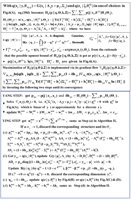
Shown in Algorithm 2 (displayed in Figure 2) is a summary of three types of adaptive algorithms for alternative ME, including NRBF and ENRBF as special cases. The implementation is almost the same for three types of learning, except taking different values of h_{j t,}. Considering k individual substructures, each has a local measure H_t( )Q_j on its fitness to a coming sample x_t and the parameters Q_j are updated by updating rules with same format to three types of learning. The updating rules are obtained from the gradientÑ_Q Q

jH_t( )_j either directly or in a modified direction that has a positive projection on this gradient, as explained in Figure 3(E). According to Figure 3(A), each updating direction is modified by

h_{j t,} on its direction and step size.

We get a further insight at a special case that h_x =0, h_z =0 (thus Step (d) discarded). The first al- locating scheme is h_{j t,} =p_{j t,} = p (j_t | )Q = p(j z x| , )_{t t} , i.e., same as the E step in Algorithm I. Actually, Algorithm II at this setting is an adaptive EM algorithm for ML learning (Xu, 1998). The second scheme only takes values at the winner and the rival, while the negative value of h_{j t,} =p_{j t,} = -g reverses the updating direction such that the rival is de-learned a little bit to reduce its fitness H_t( )Q_r to the current sample x_t. It extends the RPCL learning for NRBF from a two stage implementation (Xu, Krzyzak, &Oja, 1992&93) to an improved implementation that updates all the unknowns jointly (Xu, 1998). One prob- lem to the RPCL learning is how to choose an appropriate γ > 0. The third scheme h_{j t,} =p_{j t,}(1+dh_{t j,} ) shares the features of both the EM learning and RPCL learning without needing a pre-specified γ > 0, which is derived from the BYY harmony learning to be introduced in the sequel.

BYY HARMONY LEARNING: FUNDAMENTALS

As shown in the left –top corner of Figure 4, a set X = {x}of samples are regarded as generated via a top-down path from its inner representation R={Y, }Q , with a long term memory Θ that is a collec- tion of all unknown parameters in the system for collectively representing the underlying structure of X, and with a short term memory Y that each element y ∈ Y is the corresponding inner representation of one element x ∈ X. A mapping R®X and an inverse X®R are jointly considered via the joint

distribution of X, R in two types of Bayesian decomposition. In a compliment to the famous ancient Ying-Yang philosophy, the decomposition of p(X, R) coincides the Yang concept with a visible domain p(X) for a Yang space and a forward pathway by p( | )R X as a Yang pathway. Thus, p(X, R) is called Yang machine. Also, q(X, R) is called Ying machine with an invisible domain q(R) for a Ying space and a backward pathway by q(X | R) as a Ying pathway. Such a Ying-Yang pair is called Bayesian Ying-Yang (BYY) system. It further consists of two layers. The front layer is itself a Ying-Yang pair for X®Y and Y®X. The back layer supports the front layer by a priori q( | )Q X , while p(R | X) consists of the posteriori p( | , )Q X X that transfers the knowledge from observations to the back layer.

The input to the Ying Yang system is through p( |X Q =_x) p( |X X_N, )h obtained from a sample set X_N ={ }x_{t t}^N₌₁, e.g., p( |X X_N, )h =G(X X- _N | ,0 h I² ). To build up an entire system, we need to Figure 2. Algorithm 2: Adaptive learning algorithm for alternatve ME and NRBF nets

design appropriate structures for the rests in the system. Different designs perform different learning tasks and thus typical learning models are unified under a general framework. As shown in Figure 4, designs are guided by the following three principles, respectively:

• Least Redundancy Principle Subject to the nature of learning tasks, q(R) should be in a struc- ture for the inner representation of X_N encoded with a redundancy as least as possible. First, the number of variables and parameters of R= { , }Y Q should be as less as possible, which is itself the model selection task that is beyond the task of design. Second, the dependences among these Figure 3. Allocating schemes, typical examples, and gradient based updating

variables should be as least as possible, which is possibly or at least partly to be considered. E.g., when Y consists of multiple components Y = {Y^{( )j} }, we design q( | )Y Q =

Õ

_jq Y( ^{( )j} |^q_y^{( )j} )^.

• Divide and Conquer Principle Subject to the representation formats of X and Y, a complicated mapping Y ®X is modeled by designing q( | )X R =q( | , )X Y Q via a mixture of a number of simple structures. E.g., we may design q( | , )X Y Q via a mixture of a number of linear regres- sion featured by Gaussians of Y conditional on X. In some situation, it is not necessary to design q(R) and q(X | R) separately. Instead, we design q(X, R) (especially q( , ,X Y Q_q)) via a single parametric model as a whole but still attempting to follow the above two principles. One example is a product Gaussian mixture, as the one encountered in Type B of Rival penalized competitive learning (see Xu, 2007b). In general, we may consider an integrable measure M( , ,X Y Q_q) by Figure 4. Bayesian Ying-Yang system and best harmony learning

q( , ,X Y Q_q)=M( , ,X Y Q_q) /

ò

M( , ,X Y Q_q)d dX Y

• Uncertainty Conversation Principle In a compliment to the Ying-Yang philosophy, Ying is pri- mary and thus is designed first, while Yang is relatively secondary and thus is designed basing on Ying. Moreover, as illustrated by the Ying-Yang sign located at the top-left of Figure 4, the room of varying or dynamic range of Yang should balance with that of Ying, which motivates to design p(X, R) (in fact, only p(R | X) because we have p( |X Q =_x) p( |X X_N, )h already) under a prin- ciple of uncertainty conversation between Ying-Yang. In other words, Yang machine preserves a varying room or dynamic range that is appropriate to accommodate uncertainty or information contained within the Ying machine. That is U p( ( , ))X R =U q( ( , ))X R under a uncertainty mea- sure U(p), in one of the choices within the table in Figure 4. Since a Yang machine consists of two components p( | ) ( )R X p X , we may consider one or both of the uncertainty conversations as follows:

U p( ( | ))R X =U q( ( | )),R X q( | )R X =q( , ) / ( )X R q X and U p( ( ))X =U q( ( )), ( )X q X =

ò

q( , )X R Rd

The above uncertainty conservation may occur at three different levels. One is likelihood based con- servation that the structure of Yang machine gets a strong link to the ones of Ying machine. Considering

p L | _{L X}

L ( X q, _| )

å

^{= 1}, the Yang structure is actually given by the Bayesian inverse of Ying machine p L |( X,q_{L X|} )=q( , ) /X R

å

_Lq( , )X R , further examples are referred to Tab.2 of (Xu, 2008a). A less constrained link is provided by a Hessian based conversation, i.e., a conservation on local convexity, which is applicable to Y, Θ of real variables. This is a type of local information conservation, e.g., Fisher information conservation. The most relaxed conservation is based on a collective measure instead of details, e.g., Shannon entropy.

Again, we use S_k(Q_k) to denote a family of system specifications, with k featured by the scale or complexity for representing R, which is contributed by the scale k_Y for representing Y and an effec- tive number standing for free parameters in Q_k. An analogy of this Ying Yang system to the Chinese ancient Ying-Yang philosophy motivates to determine k and Q_k under the best harmony principle, mathematically to maximize

H p q( || , , )k X =

ò

p( | ) ( |R X p X X_N, )ln[ ( | ) ( )]h q X R R X Rq d d . ₍₈₎

On one hand, the maximization forces q( | ) ( )X R Rq to match p( | ) ( |R X p X X_N, )h . In other words, q( | ) ( )X R Rq attempts to describe the data p( |X X_N, )h in help of p(R | X), which uses actually q( )X =

ò

q( | ) ( )X R R Rq d ^{to fit p( |X XN, )h} not in a maximum likelihood sense but with a promising model selection nature. Due to a finite size of X_N and structural constraint of p(R | X), this matching aims at (but may not really reach) q( | ) ( )X R R = pq ( | ) ( |R X p X X_N, )h . Still we get a trend at this equality by which H p q( || , , )k X becomes the negative entropy, and its further maximization is minimizing the system complexity, which consequently provides a model selection nature on k.

At the first glance, one may feel the formulae eqn.(8) somewhat familiar. In fact, its degenerated case with R vanished leads to H p q( || )=

ò

p( )ln ( ) .^X q ^{X X}d ^{With p( )X =p( |X XN, )h} at h = 0 and q( )X =q( | )X Q , maximizing this H p q( || ) becomes max ln (_Q q X_N | )Q , i.e., maximum likelihood (ML) learning. The situation with p(X) beyond p( |X X_N, )h was also explored in the signal processing literature, via min_{q( )X}-H p q( || ) under the name of Minimum Cross-Entropy (Minxent). It was noticed that min_{p( )X}-H p q( || ) leads to a singular result that p( )X =d(X X- ^*),X^* =arg max ln ( | )_X q X Q , which was regarded as irregular and not useful. Instead, efforts were turned to minimizing the classic Kullback–Leibler divergence KL p q( || )=H p p( || )-H p q( || ) with respect to p, which pushes p to match q and thus the above singular result is avoided. Moreover, if p is given, min_{q( )X} KL p q( || ) is still equivalent to min_{q( )X}-H p q( || ). Thereafter, Minimum Cross-Entropy is usually used to refer this

minKL p q( || ).

Interestingly, with an inner representation R considered in the BYY system, the scenario becomes different from the above classic situation. With p( )X =p( |X X_N, )h fixed, max_{p( )X} H p q( || ) is made with respect to only p(R | X), which is no longer useless but responsible to the promising least complex- ity nature discussed after eqn.(8). In other words, maximizing max ( || )H p q with respect to unknowns not only in Ying part q(X, R) but also in Yang part p(X, R) makes the Ying-Yang system become a best harmony. Alternatively, we may regard such a mathematical formulation as an information theoretic interpretation of the ancient Ying Yang philosophy.

In implementation, H p q( || , , )k X =

ò

p( |Q X_N) ( || , , , )H p q Q k X Qd can be approximated via a Taylor expansion of H p q( || , , , )Q k X around Q^* up to the second order as follows:

( || , , ) ( | _N) ( || , , , ) H( ^*,k, ) 0.5 ( ),

H p q k p X H p q k d p || q, d_k

q d

arg max ( || , , , ), ) [ ( )] , ,

* * * T * *

H p k k( Tr ( ) ( )( )

H p q( || , , , )Qk X =H p q₀( || , , , )Q k X +ln ( | ),q Q X

0( || ,

H p q Θ k ), ,Ξ =

∫

^{p Y X( | , y|x) (X X| N, )h ln [ (q X Y| , x|y) (Y| y)]d d}X Y ln ( ),⁺ q h

, Ξ = ∇2 H(p || q, ,k, =

∫

( |^XN) ^{d , =}

∫

^{( − )( − )T ( |XN)d .} (9) The maximization of H p q( || , , )k X consists of an inner maximization that seeks the best harmony among the front layer Ying-Yang supported by a priori q( | )Q X and an outer maximization that seeks the best harmony of the entire Ying Yang system with d ( )_k X taken in consideration for the interaction between the front and back layers.

BYY HARMONY LEARNING: CHARACTERISTICS AND IMPLEMENTATIONS Systematically considering two pathways and two domains coordinately as a BYY system under a prob- ability theoretic ground and designing three system components under the principles of least redundancy,

divide-conquer, and uncertainty conversation, respectively. BYY harmony learning is different not only from cognitive science motivated adaptive resonance theory (Grossberg, 1976; Grossberg & Carpenter, 2002) and the least mean square error reconstruction based auto-association (Bourlard & Kamp, 1988) and LMSER self-organization (Xu, 1991 & 93), but also from those probability theoretic approaches that either merely consider a bottom-up pathway as the inverse of a top-down pathway (e.g., Bayes- ian approaches), or approximate such inverses for tackling intractable computations (e.g., Helmholtz machine, varianional Bayes, and extensions). Mathematically implementing the Ying-Yang harmony philosophy, in a sense that Ying and Yang not only matches each other but also seeks a best match in a most compact way, by determining all unknowns in a BYY system via maximizing the functional of

H p q( || , , )k X , with the model selection nature explained after eqn.(8).

Readers are further referred to (Xu, 2007a) for a systematical overview on relations of Bayesian Ying Yang learning to a number of typical approaches for either or both of parameter learning and model selection, covering the following aspects:

• Best Data Matching perspective, for modeling a latent or generative model and involving ML, Bayesian, AIC, BIC, MDL, MML, marginal likelihood, etc;

• Best Encoding perspective, for encoding inner representation by a bottom-up pathway (or called a transformation / recognition / representative model) and involving INFOMAX, MMI based ICA approaches and extensions;

• Two Pathway Perspective, involving information geometry based em-algorithm, Helmholtz Machine, variational approximation, and bits-back based MDL, etc.

• Optimal Information Transfer Perspective, involving MDL, MML, and bits-back based MDL, etc.

The model selection nature of maximizing H p q( || , , )k X can also be observed from its gradient follow with the Yang path in a Bayesian structure p( | )R X =q( | ) ( ) / ( )X R Rq q X , q(X) =

ò

q( | ) ( )X R R Rq d ^. It follows that we have

dH p q p _L dL p _N h d d

L

( || , , ) ( | )[ ( , )] ( , ) ( | , ) , ( ,

k R X X R X R X X X R

X

X =

ò

¹+^d

d RR)=^L( , )X R -

ò

^p( | ) ( , ) ,R X^L X R R^{d and L}( , )X R =ln[ ( | ) ( )]^q X R R^{q (10a)} Noticing that L(X, R) describes the fitness of an inner representation R on the observation X, we observe that d_L( , )X R indicates whether the considered R fits X better than the average of all the pos- sible choices of R. Letting d_L( , )X R = 0, the rest of dH p q( || , , )k X is actually the updating flow of the M step in the EM algorithm for the maximum likelihood learning (McLachlan & Geoffrey,1997).

Usually d_L( , )X R ¹ 0, i.e., the gradient flow dL(X, R) under all possible choices of R is integrated via weighting not just by p(R | X) but also by a modification of a relative fitness measure 1 +d_L( , )X R . If d_L( , )X R > 0, updating goes along the same direction of the EM learning with an increased strength.

If 0>d_L( , )X R > -1, i.e., the fitness is worse than the average and the current R is doubtful, updating still goes along the same direction of the EM learning but with a reduced strength. When - >1 d_L( , )X R , updating reverses the direction of the EM learning and actually becomes de-learning. In other words, the BYY harmony learning shares the same nature of RPCL learning but with an improvement that

there is no need on a pre-specified de-learning strength γ > 0, as previously discussed in Figure 3(A) on a special case of NRBF & ME with R = { , }j Q , where p( | )[R X 1 +d_L( , )]X R is simplified into

p_{j t,}(1 +dh_{t j,} ) and d_L( , )X R into dh_{t j,} .

More specifically, the model selection nature of Bayesian Ying Yang learning possess the following favorable promising features.

The conventional model selection approaches aim at model complexity conveyed at either or both

•

of the level of structure S_k and the level of parameter set Q. This task is difficult to estimate, usu- ally resulting in some rough bounds. Bayesian Ying Yang learning considers not only the levels of S_k and Q but also the level of short memory representation Y by the front layer of BYY system in Figure 4(a). That is, the scale k of the BYY system is considered with the part k_Y for representing Y, while the rest part, contributed by S_k and Q, is estimated via ln q(Q|X) and d_k( )X in eqn.(9), which is along a line similar to the above conventional approaches. Interestingly, the part k_Y is modeled via q(Y|Q_y) in H p q₀( || , , , )Q k X , which is estimated more accurately than the rest part.

Promisingly, the model selection problems of many typical learning tasks can be reformulated into selecting merely the k_Y part in a BYY system (Xu, 2005). Therefore, the resulted BYY harmony criterion J(k) shown by the left one of Figure 4(b) may considerably improve the performances by typical model selection approaches, which has been shown by in experiments (Shi, 2008).

Even interestingly, this

• k_Y part associates with a set _{y y} of parameters on which there ex- ists an indicator ( )_y . Maximizing H p q₀( || , , , )Q k X will exert a force that pushes ( )_y 0, which means that its associated contribution to k_Y can be discarded. E.g., each j of k values associates with one α_j, we can discard a structure if its correspondent r a( )_j =a_j ® 0. As a result, k effectively reduces to k − 1. As illustrated on the right of Figure 4(b), a_j ® 0 means its contribution to J k( ) is 0, and a number of such parameters becoming 0 result in that J k( ) has effectively no change on a range [ˆ, ]k k . Also, each dimension y⁽ⁱ⁾ of q y( | )q_j^y associates with its variance l_j and this dimension can be discarded if l_j ® 0. As illustrated beyond k on the right of Figure 4(b), such a parameter becoming 0 contributes to J k( ) by -¥. As long as k_Y is initialized at a big enough value, ˆk can be found as an upper bound estimate of k^*. That is, an automatic model selection is incurred during parameter learning. Details are referred to Sec.2.3 of (Xu, 2008a&b).

The separated consideration of

• k_Y from the rest of k also provides a general framework that in- tegrates the roles of regularization and model selection, such that not only the automatic model selection mechanism on k_Y can avoid the previously mentioned disturbance by a regularization with an inappropriate priori q( | )Q X , but also imprecise approximations caused by handling the integrals may be alleviated via regularization. Specifically, model selection is made via q( |Y Q_y) in Ying machine, while regularization is imposed in Yang machine via designing its structure un- der a uncertainty conservation principle given at the bottom of Figure 4 and making data smooth- ing regularization via p( )X =p( |X X_N, )h with h ¹ 0 that takes a role similar to regularization strength, while the difficulty of the conventional regularization approaches on controlling this strength has been avoided because an appropriate h ¹ 0 is also determined during maximizing

H p q( || , , , )Q k X .

At a first glance, a scenario with q( |Y Q_y) is seemly involved also in several typical learning ap- proaches, especially those with an EM like two pathway implementation, such as the EM algorithm implemented ML learning (Redner & Walker, 1984), information geometry based em-algorithm (Amari, 1995), Helmholtz Machine (Hinton, Dayan, Frey, & Neal, 1995; Dayan, 2002), variational approxima- tion (Jordan, Ghahramani, Jaakkola, & Saul, 1999), the bits-back based MDL (Hinton & Zemel, 1994), etc. Actually, these studies have neither put q( |Y Q_y) in a role for describing k_Y nor sought for the above nature of automatic model selection. Instead, the role of q( |Y Q_y) in these studies is estimating

x|y y

( ) ( | , ) ( | )

q X q X Y q Y dY in a ML sense or approximately, which is similar to the one in Bayes- ian Kullback Ying Yang (BKYY) learning that not only accommodates a number of typical statistical learning approaches (including these studies) as special cases but also provides a bridge to understand the relation and difference from the best harmony learning by maximizing H p q( || , , , )Q k X in eqn.(8).

Proposed in (Xu,1995), BKYY learning performs a best Ying Yang matching by minimizing:

KL p q p p h p p h

q q d

N

( || , , ) ( | ) ( | , )ln ( | ) ( | N, ) ( | ) ( )

k R X X X R X X X

X R R X

X =

ò

^ddR- ( || , , ),^{H p q k} X (10b)

that is, a best Ying Yang harmony includes not only a best Ying Yang matching as a part but also mini- mizing the entropy or the complexity of a Yang machine. In other words, it seeks a Yang machine that not only best matches the Ying machine but also keeps itself in a least complexity.

Considering a learning system in a Ying-Yang pair naturally motivates to implement the maximization of H p q( || , , , )Q k X or the minimization of KL p q( || , , , )Q k X by an alternative iteration of

• Yang step: fixing all the unknowns in the Ying machine, we update the rest of the unknowns in the Yang machine (after excluding those common unknowns shared by the Ying machine);

• Ying step: fixing those just updated unknowns in the Yang step, we update all the unknowns in the Ying machine.

Not only this iteration is guaranteed to converge, but also it includes the well known EM algorithm and provides a general perspective for developing other EM-like algorithms.

Recalling eqn.(9), the maximization of H p q( || , , , )Q k X can be approximately decoupled into an inner maximization for the best harmony among the front layer supported by a priori q( | )Q X and an outer maximization for interaction between the front and back layers. Thus, we have the following two stage implementation:

k k

K ⁽⁰⁾

( ) ( 1)

( ) ( ) ( ) ( ) ( )

Stage I enumerate each , initialize and iterate : ( ) arg max/incr ( || , , , ),

( ) arg max/incr [H( , , ) ( )], , 1,

t t

t t t t t

a H p q

b p || q, d_k

k

k k

( ) ( ) ( ) * *

*

( ) ( ) ( , , after convergence we get , ; Stage II argmin ( ), ( ) ( ) 0.5 ( ).

t T t t

f

f

d n

J J J n

k k

k k

)

k  k (11a)