雷射捕捉誘發水中PNIPAM 分子相轉變動態之研究藉由光學顯微技術及時間分析螢光顯微光譜技術

國立交通大學

應用化學系碩士班

碩士論文

雷射捕捉誘發水中 PNIPAM 分子相轉變動態之研究藉由光

學顯微技術及時間分析螢光顯微光譜技術

L a s e r - i n d u c e d p h a s e t r a n s i t i o n d y n a m i c s o f

p o l y ( N - i s o p r o p y l a c r y l a m i d e ) i n w a t e r s t u d i e d b y

o p t i c a l m i c r o s c o p y a n d t i m e - r e s o l v e d

f l u o r e s c e n c e m i c r o s p e c t r o s c o p y .

研究生: 曾綮續 (Tseng Chin-Hsu)

指導教授: 三浦篤志 博士 (Atsushi Miura)

中華明國 一百零一年 七 月

1

Abstract

Student：

Tseng Chin-Hsu

Advisor：Dr.

Atsushi Miura

M. S. Program, Department of Applied Chemistry

National Chiao Tung University

A poly(N-isopropylacrylamide) (PNIPAM) is famous thermo-responsible polymer which shows phase transition above lower critical solution temperature (LCST). PNIPAM collapses into globule from coli state where hydrated water molecules are excluded from the polymer matrix. It is considered that the phase transition behavior including dehydration process and folding change is a good example of biological polymers such as protein, therefore many studies of phase transition behavior of PNIPAM have been examined for more than couple of decades. However direct molecular dynamics of phase transition of PNIPAM is few. In this study, we studied molecular spectroscopic phase transition dynamics of PNIPAM by introducing laser trapping, optical microscopy and time-resolved fluorescence microspectroscopy with fluorescently labeled PNIPAM. We induce local phase transition around the focal spot of trapping laser by tight focusing of trapping light source under microscope. Laser-induced phase transitin behavior and its dynamics was visualized by combining with steady state and time-resolved spectroscopy.

2

aqueous solvents, H2O and D2O, revealed that clearly different phase transition

behavior. Trapping laser irradiation induced spherical particle formation at the focal spot. The size and formation time strongly depends and changes upon solvent and laser power. It is interpreted due to a thermal effect caused by an absorption of irradiated trapping laser light by the solvents. Larger absorption coefficient of H2O

than D2O enables the phase transition at lower laser power in former solution.

Based on the information of phase transition dynamics obtained by non-labeled PNIPAM, we examined phase transition dynamics of fluorescently labeled VDP-PNIPAM. Fluorescence microscopy and microspectroscopy results of phase transition dynamics of VDP-PNIPAM clearly indicate the molecular environmental change from coli to globule during phase transition with showing the peak wavelength shift of fluorescence spectra. In addition to the fluorescence spectrum under laser trapping-induced phase transition, we measured fluorescence decay during and after phase transition. Analysis of fluorescence decay curves showed the change of decay component during phase transition which also reveal dynamic change of molecular environment during phase transition.

Additionally we found an unusual two color lasers induced phase transition behavior when we introduce weak ultraviolet (UV) laser simultaneously with near infrared (NIR) trapping laser. A spherical particle formed by trapping laser irradiation

3

showed an expansion of its size when an additional weak UV light was introduced. Observed two-color laser irradiation-induced particle size expansion will be interpreted by two reasons at the moment; resonance effect and photothermal effect.

4

雷射捕捉誘發水中 PNIPAM 分子相轉變動態之研究藉

由光學顯微技術及時間分析螢光顯微光譜技術

中文摘要

研究雷射捕捉誘發 PNIPAM 相轉變於不同溶液中, H2O 及 D2O, 確實透 露出不同的相轉變過程. 雷射捕捉會誘發球形粒子於雷射聚焦點. 大小及形成 時間與溶劑及雷射強度相當有關以及會隨之改變. 這個結果說明了因溶劑吸收 雷射而產生的熱效應. H2O 的吸收係數比 D2O 大以致於相轉變可以藉由較小強

5 度的捕捉雷射來成形. 以未標定的 PNIPAM 相轉變動態過程為基準,我們觀測了被標定的 PNIPAM 分 子,VDP-PNIPAM, 的相轉變動態過程. 藉由觀測光譜波長峰值的位移,螢光顯微 及顯微光譜上的結果清楚指出了 VDP-PNIPAM 相轉變動態過程中,分子環境從直 鏈狀變為球狀的改變. 除了測量在雷射捕捉誘發相轉變條件下的螢光光譜,我們 也在過程中及結束後測量螢光強度衰退. 分析相轉變過程的螢光強度衰退也透 露出了分子環境在向轉變過程中的動態改變. 除此之外,我們發現了一個不同於以往的雙色雷射誘發相轉變現象,當我們 同時引入紅外光捕捉雷射與一道較弱的紫外光雷射. 當額外的弱紫外光雷射引 入時,藉由雷射捕捉所形成的球形粒子會大小上會發生擴張的現象. 在現階段, 這項雙色雷射誘發相轉變大小擴張的現象會以兩個說法來解釋, 共振效應及光 轉熱效應.

6

List

1. Introduction ... 14

1.1 Poly(N-isopropylacrylamide) (PNIPAM) and its phase transition behavior17 1.2 Laser trapping ... 21

1.2.1 History of laser trapping ... 21

1.3 Fluorescence microscopy/spectroscopy for phase transition dynamics study ... 24

1.4 Aim of this study ... 25

2. Experiment ... 27

2.1 Materials ... 27

2.2 Bright field transmission imaging and fluorescence imaging/spectroscopy system: ... 28

2.3 Microscopy setup: Fluorescence lifetime imaging microscopy system 32 3. Phase transition of PNIPAM induced by trapping laser ... 37

3.1 Laser trapping-induce phase transition of PNIPAM ... 37

3.2 Heating effect of glass substrate ... 42

3.3 Position dependence of PNIPAM phase transition ... 46

3.4 Summary ... 48

4. Fluorescence lifetime measurement and construction of fluorescence lifetime imaging microscopy (FLIM) system ... 50

4.1 Fluorescence from molecule. ... 51

4.2 Time-correlated single photon counting ... 53

4.3 Fluorescence lifetime imaging microscopy (FLIM) ... 59

4.4 Evaluation of Fluorescence lifetime imaging microscopy system ... 60

4.5 Summary ... 67

5. Phase transition dynamic of VDP-PNIPAM by fluorescence microscopy ... 68

5.1 Laser trapping induce phase transition of VDP-PNIPAM ... 68

5.2 Fluorescence decay dynamics of VDP-PNIPAM during phase transition ... 71

5.3 Spectra and lifetime change of VDP-PNIPAM phase transition ... 80

5.4 Spatially resolved fluorescence lifetime measurement in phase transition induced microparticle ... 90

6. Two color laser-induced phase transition of PNIPAM and VDP-PNIPAM ... 95

6.1 Blue laser induce phase transition expansion ... 95

6.2 UV laser power dependence of particle expansion in VDP-PNIPAM phase transition ... 99

7

6.3 The excitation wavelength dependence for two color effect ... 103 6.4 Proposed mechanism of two color laser induced phase transition

expansion ... 106 7. Summary ... 113 Reference ... 116

8

List of Figure

Figure 1.1 Chemical structure of PNIPAM. ... 18 Figure 1.2 Schematic drawing of PNIPAM phase transition. ... 19 Figure 1.3 Focus laser beam induced molecular assembly formation of PNIPAM in aqueous solution. Figure from reference [33] ... 20 Figure 1.4 Schematic diagram of ray optics for typical trapping which the refraction index of particle is larger than that of the medium. Redraw from [42]. ... 23 Figure 2.1 Chemical structure of (a) PNIPAM and (b) VDP-PNIPAM) ... 28 Figure 2.2 (a) Schematic diagram of microscope setup for bright field transmission imaging and wide-field fluorescence imaging/spectroscopy. (b) A drawing of sealed glass chamber. ... 32 Figure 2.3 Schematic diagram of fluorescence lifetime imaging microscopy system. 35 Figure 2.4 System of fluorescence measurement: (a) A picture of TCSPC system and (b) cabling diagram. ... 36 Figure 3.1 Local phase transition induced by laser trapping in (a) ~ (d) H2O and (e) ~

(f) D2O. Laser power was 725 mW. Scale bar = 10 μm. Time indicated in the images

corresponds the irradiation time of trapping laser. ... 39 Figure 3.2 Trapping laser power dependent formed particle size difference. The symbols show PNIPAM in H2O (▲) and D2O (■) and VDP-PNIPAM in H2O (◆)

and D2O (★), respectively. ... 40

Figure 3.3 Phase transition time change upon laser power. The symbols show PNIPAM in H2O (▲) and D2O (■) and VDP-PNIPAM in H2O (◆) and D2O (★),

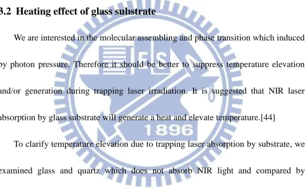
respectively. ... 40 Figure 3.4 Phase transition-induced microparticle formation in H2O with (a) ~ (c)

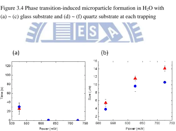
glass substrate and (d) ~ (f) quartz substrate at each trapping power. ... 44 Figure 3.5 Power dependence of (a) particle size and (b) phase transition time in H2O

solution. The symbols show glass (▲) and quartz (●). ... 44 Figure 3.6 Power dependence of phase transition time in H2O solution with glass (■)

and quartz (▲) substrate. ... 45 Figure 3.7 Power dependence of (a) phase transition time and (b) particle size formed in the glass (■) and quartz (◆) chamber. PNIPAM/D2O solution was used. ... 45

Figure 3.8 Position dependence of (a) phase transition time and (b) particle size with glass substrate(■), and (c) phase transition time and (d) particle size with quartz (▲) substrate. PNIPAM/H2O solution was used. Trapping laser powers for glass and

9

Figure 4.1 Jablonski diagram. S0 and S1 are ground and lowest excited singlet state,

respectively. T1 is lowest excited triplet state. The k means rate constant for ka:

absorption; kr: fluorescence kr’: phosphorescence, knr, knr’: non-radiative deactivation,

kisc : intersystem crossing ... 52

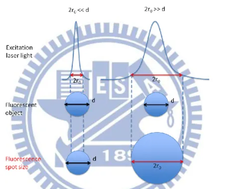
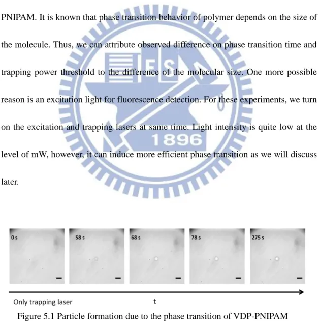
Figure 4.2 Principle of TCSPC. (a) Variation of an arriving time of emitted photon from fluorophore and (b) a histogram constructed from the photons came after the excitation pulse. This histogram is fluorescence decay curve. ... 56 Figure 4.3 Schematic diagram of TCSPC system. From [45] ... 58 Figure 4.4 Conceptual drawing showing difference of intensity imaging (left) and lifetime imaging (FLIM, right). of FLIM. From [46] ... 60 Figure 4.5 Pictures of mixed PS beads monolayer on the grass observed by (a) bright-field, (b) fluorescence intensity, (c) fluorescence lifetime, and (d) superimposed image of (a) and (c). The lifetimes of ~4 ns (red) and ~2 ns (green) correspond to the fluorescence lifetime of No.2 and No. 4, respectively. A 40x long working distance objective lens was used for both bright field and FLIM images.. ... 63 Figure 4.6 Beam spot size of excitation light source determine the fluorescence spot size. Beam spot size is smaller (left) and larger (right) than that of fluorescent object. ... 65 Figure 4.7 Fluorescence intensity image of 40 nm fluorescent beads and cross-sectional line profile along the lines in the image. The picture size is 5x5 m2. ... 66 Figure 5.1 Particle formation due to the phase transition of VDP-PNIPAM induced by trapping laser in H2O solution. Trapping laser power was 200 mW. Scale bar = 10 μm.

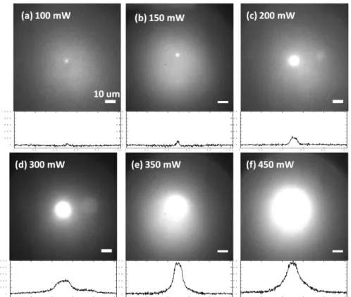
... 69 Figure 5.2 Fluorescence images of particle formed by laser trapping. Values in the images indicating trapping laser power used for inducing the phase transition. VDP-PNIPAM was in H2O. Excitation wavelength was 325 nm. ... 70

Figure 5.3 Phase transition time change depends on trapping laser power. A 325 nm fluorescence excitation laser was irradiated simultaneously with trapping laser. VDP-PNIPAM was in H2O solution. ... 71

Figure 5.4 Fluorescence decay curve of VDP-PNIPAM in H2O before (green) and

during (black) phase transition. Excitation wavelength and laser power was 375 nm and 12 W. Trapping laser power was 200 mW. ... 74 Figure 5.5 Fluorescence decay curves measured during phase transition process at (a) particle formation and (b) particle disappearance. Laser trapping power was 200mW. Fluorescence excitation was at 375 nm with 12 W ... 75 Figure 5.6 Fluorescence images obtained simultaneously with fluorescence decay measurements in particle formation process shown in Figure 5.5a. Laser trapping

10

power was 200mW. Fluorescence excitation was at 375 nm with 12 W. Scale bar is 10 μm. ... 76 Figure 5.7 Fluorescence images obtained simultaneously with fluorescence decay measurements in particle disappearance process shown in Figure 5.5b. Laser trapping power was 200mW. Fluorescence excitation was at 375 nm with 12 W. Scale bar is 10 μm. ... 76 Figure 5.8 Fluorescence spectra measured simultaneously with fluorescence decay measurements in particle formation process shown in Figure 5.5a. The spectrum shifted from 480 nm to 455 nm is seen in the figure. Laser trapping power was 200mW. Fluorescence excitation was at 375 nm with 12 W. ... 77 Figure 5.9 Fluorescence spectra measured simultaneously with fluorescence decay measurements in particle disappearance process shown in Figure 5.5b. The spectrum shifted from 450 nm to 480 nm is seen in the figure. Laser trapping power was 200mW. Fluorescence excitation was at 375 nm with 12 W. ... 77 Figure 5.10 Lifetime and amplitude values obtained from the decay curves showed in Figure 5.5a, particle formation process. Vertical line in the graph indicates when phase transition observed. The symbols mean the lifetime (■) and amplitude (★) value for long component and lifetime (○) and amplitude (△) value for short component. .... 79 Figure 5.11 Lifetime and amplitude values obtained from the decay curves showed in Figure 5.5a, particle formation process. The symbols mean the lifetime (■) and amplitude (★) value for long component and lifetime (○) and amplitude (△) value for short component. ... 79 Figure 5.12 Temperature dependence of VDP-PNIPAM spectrum in H2O solution. .. 82

Figure 5.13 Temperature dependence of VDP-PNIPAM spectrum in D2O solution. .. 83

Figure 5.14 Temperature dependent of peak wavelength of spectrum. The horizontal value is compensated temperature. ... 83 Figure 5.15 Spectrum detected at different temperature in H2O solution. Excitation

was at 375 nm. Spectrum obtained under trapping condition was shown together. Trapping laser power was 200 mW. ... 85 Figure 5.16 Spectrum detected at different temperature in D2O solution. Excitation

was at 375 nm. Spectrum obtained under trapping condition was shown together. Trapping laser power was 200 mW. ... 85 Figure 5.17 Decay curves at different temperature in H2O solution. Excitation was at

375 nm. Decay obtained under trapping condition was shown together. Trapping laser power was 200 mW. ... 86 Figure 5.18 Decay curves at different temperature in D2O solution. Excitation was at

375 nm. Decay obtained under trapping condition was shown together. Trapping laser power was 700 mW. ... 86

11

Figure 5.19 Temperature dependent fluorescence lifetime change for H2O (red, purple)

and D2O (blue, green) shown in Figs. 5.16 and 5.17. Solid and open symbol mean the

long and short lifetime values. ... 87 Figure 5.20 Fluorescence lifetime change was plotted against peak wavelength of simultaneously measured fluorescence spectra. All data for H2O and D2O are

summarized. The symbols mean the same as in Figure 5.18. ... 87 Figure 5.21 The decay curve of VDP-PNIPAM in solution at 25 ˚C fitted by one and two decay components. ... 89 Figure 5.22 Schematic drawing of position dependent lifetime experiment in phase transition particle. ... 90 Figure 5.23 The picture of excitation position dependence lifetime measurement in H2O solution. Scale bar = 10 μm, Cursor position is focus position of excitation laser.

... 92 Figure 5.24 Decay curves measured at different position. VDP-PNIPAM was dissolved in H2O. Phase transition was induced by 200 mW trapping laser.

Fluorescence was excited by 375 nm at 12 W. ... 93 Figure 6.1 Phase transition of VDP- PNIPAM induced by (a) only trapping laser and (b) additional UV laser and (c) again only trapping laser. VDP-PNIPAM in H2O

solution was used. Trapping laser power was 200 mW and UV laser power was 15 mW. ... 96 Figure 6.2 Particle size change by turn on/off of 325 nm laser (upper panel) and size at each conditions (lower panel). ... 97 Figure 6.3 Phase transition of PNIPAM induced by trapping laser (a) and UV and trapping laser (b) in H2O solution. Trapping laser power was 200 mW and UV laser

power was 15 mW. ... 98 Figure 6.4 Particle size change of PNIPAM by turn on/off excitation laser in H2O

solution (upper panel). Size at each conditions (lower panel). ... 98 Figure 6.5 Pictures of phase transition particles at each excitation laser power in H2O

solution. (a) ~ (g) are the particles formed by trapping laser and their corresponding two colors laser expansion phase transition images are in (h) ~ (n). Trapping laser power= 200 mW. ... 101 Figure 6.6 Particle size change at each excitation laser power in H2O solution.

Trapping laser power =200 mW. (■) for trapping laser and (●) for two color lasers irradiation. ... 102 Figure 6.7 Pictures of phase transition particles at each excitation laser power in D2O

solution. (a) ~ (f) are the particles formed by trapping laser and their corresponding two colors laser expansion phase transition images are in (g) ~ (l). Trapping laser power =600 mW. ... 102

12

Figure 6.8 Particle size change at each excitation laser power in D2O solution.

Trapping laser power = 600 mW. (■) for trapping laser and (●) for two color lasers irradiation. ... 103 Figure 6.9 Absorption and emission spectrum of VDP-PNIPAM in H2O solution.

Concentration= 0.01 wt %. Excitation wavelength for emission spectrum: 325 nm. 104 Figure 6.10 Wavelength dependence of phase transition expansion in H2O solution.

(a)~ (d) are phase transition induced by only NIR trapping laser. (e) ~ (f) are phase transition irradiated by second light with 325, 375, 405 and 488 nm, respectively. Graph (d) and (f) are recorded in D2O solution. Trapping laser power was 200 mW in

H2O and 600 mW in D2O. All the excitation laser power was 15 mW. ... 105

Figure 6.11 Excitation wavelength dependence of VDP-PNIPAM phase transition expansion. The excitation light power at each wavelength is 15 mW. ... 106 Figure 6.12 Absorption spectrum of VDP-PNIPAM. An arrow in the figure indicates the wavelength of UV laser used in our experiments which has large overlap with electronic transition band of labeled fluorophore. ... 109 Figure 6.13 Schematic drawing of photothermal effect induced by multiphoton absorption in excited state. Here we omit relaxation path through triplet state in this scheme. ... 112

13

List of Table

Table 3.1 Phase transition time and particle size in H2O and D2O solution. ... 41

Table 3.2 The PNIPAM phase transition time and size at each trapping laser power in H2O solution ... 46

Table 3.3 The PNIPAM phase transition time and size at each trapping laser power in D2O solution ... 46

Table 3.4 Phase transition time and size at different position of the sample chamber. 48 Table 4.1 The fluorescence beads list. ... 61

Table.5.1 The VDP-PNIPAM phase transition time each trapping laser power in H2O solution. ... 71

Table 5.2. Fluorescence lifetime decay parameters of VDP-PNIPAM before (green) and during (black) phase transition. ... 74

Table 5.3 Peak wavelength of VDP-PNIPAM at different temperature. Temperature value are compensated values. ... 84

Table 5.4. Temperature dependent peak wavelength and lifetime value change. ... 88

Table 5.5 Lifetime components of fitting analysis shown in Fig. 5.24. ... 89

Table 5.6. The lifetime value of decay curve at different position far from phase transition center. ... 93

Table 6.1 Mean size value of phase transition under each excitation power. ... 101

Table 6.2 Mean size value of phase transition under each excitation power. ... 103

14

1.

Introduction

To study dynamic structural change or phase transition of biological molecules, it is indispensable to understand conformational and hierarchic structure change at molecular level during its function emerging process with high space- and time-resolution. For instance, protein structure can be represented by α-helix, β-sheet, and so on by changing surrounding condition such as temperature, pressure, salt and enzyme concentration, and electric potential of membrane etc. However direct investigation of structural transition dynamics is experimentally hard, thus varieties of stimuli-responsive polymers have been used for such kind of studies. A poly(N-isopropylacrylamide) (PNIPAM) is one of such stimuli-responsive polymer.

As is well established, PNIPAM in aqueoussolution exhibits a structural change upon increasing the temperature beyond a lower critical solution temperature (LCST) at 32˚C.[1] As a consequence, NIPAM solutions show phase transition above the LCST. This fascinating thermo-responsive behavior stimulated extensive studies of PNIPAM solutions and gels for the preparation of stimuli-responsive devices and formulations with potential biomedical applications.[2, 3]

A molecular mechanism behind the phase transition of PNIPAM is considered due to the dehydration in the polymer matrix and, therefore, less hydrogen bonding

15

between amide moiety and water molecule which renders water a poor solvent for the chain. Hence, the polymer chain existing as an extended coil collapses into a globular form above the LCST with a high degree of tight contact among the hydrophobic side chains. As established primarily by calorimetric studies, [4, 5] the PNIPAM chain in the collapsed state is composed of globular domains of a size in the order of molecular weight (MW ~104) with small extended portions of the chain in between them. This scenario is well supported by a wealth of experimental results by light scattering [6, 7], NMR [8-10] and fluorescence spectroscopies [11, 12]. Macroscopically, the solution turns turbid above the LCST, even for short (MW ~104) chains of PNIPAM.[13, 14] This latter observation indicates that intermolecular aggregation also occurs, a scenario that is further corroborated by elegant fluorescence experiments [15] with doubly labeled polymer chains and by detailed light-scattering studies.[16, 17] There are also indications that at finite concentrations of PNIPAM can form stable multi-chain aggregates which are reported to as ‘‘mesoglobules’’.[18, 19]

In contrast to the wealth of observations underlying the broad structural consensus, there is a remarkable lack of understanding of PNIPAM phase transition on the time course of molecular events in the bulk solutions. Quite little is known about the dynamic behavior of phase transition and separation of PNIPAM. Kinetic studies were performed in the dense (5–90 wt.%) regime by calorimetry investigations

16

indicated a demixing/remixing process that may proceed on the <100 s time scale with the remixing being slower than the demixing [20] and ultrasonic attenuation studies revealed dynamics of ambiguous origin on the minutes-to-hours time scale.[21]

In 2006, Yushmanov et al. performed a temperature-jump 1H NMR study on PNIPAM to access the dynamic behavior of the phase transition/separation in an aqueous polymer solution (1wt.%).[22] Their results revealed that phase mixing/demixing, i.e. phase separation, was completed within a few seconds. In order to elucidate a dynamic behavior of the phenomena, however, further detailed investigation with better time resolution is necessary. Tsuboi et al. reported that the phase separation dynamics of PNIPAM in aqueous solutions by means of a laser temperature-jump (T-jump) technique.[23] They revealed that the time constant of the phase separation of the polymer solution was proportional to the square of the hydrodynamic radius of the polymer.

However direct spectroscopic approach to study the phase transition dynamics of polymer solutions is usually difficult, since coiled and globular states are hardly distinguished spectroscopically. To overcome this experimental difficulty, we employ a PNIPAM co-polymerized with fluorescent probe in this study [24-26]. A use of a fluorescent probe molecule is effective for studying the molecular motion of PNIPAM

17

systems, as Winnik et al. have demonstrated previously.

1.1 Poly(N-isopropylacrylamide) (PNIPAM) and its phase transition

behavior

PNIPAM is one of the most widely studied thermoresponsive polymer. PNIPAM is a chemical isomer of poly-leucine, in that it has the polar peptide group in its side chain rather than in the backbone.[27] PNIPAM consists of a hydrocarbon backbone with hydrophilic and hydrophobic moieties in the form of carboxyl, amide and isopropyl groups as shown in Figure 0.1 Chemical structure of PNIPAM.. In aqueous solution, PNIPAM displays a LCST at 32˚C; at this temperature it undergoes a sharp and reversible coil-to-globule phase transition from a hydrophilic to a more

hydrophobic state, forcing water out from the matrix. This phenomenon occurs due to the domination of entropic effects (displacement of water from the polymer matrix) over enthalpic effects (formation of hydrogen bonds between polymer and water molecules) as the temperature increaes above the LCST.[28, 29]

18

Below LCST, PNIPAM chains exist in an extended coil conformation, and solvation is driven by the enthalpic gain from intermolecular hydrogen bonding between the PNIPAM chains and water molecules as shown in left side in Figure 0.2.[2] As the temperature is increased towards the LCST, intramolecular hydrogen bonding between carboxyl and amide groups on the PNIPAM chains result in the interruption of hydrogen bonding of these groups with water molecules, ultimately resulting in the chain adopting a collapsed conformation, driving out the water, and causing the polymer to precipitate in the solution as shown in right side in Figure 0.2. These interesting properties of PNIPAM and its copolymers make them applicable to a diverse range of pharmaceutical and biomedical applications [30, 31].

19

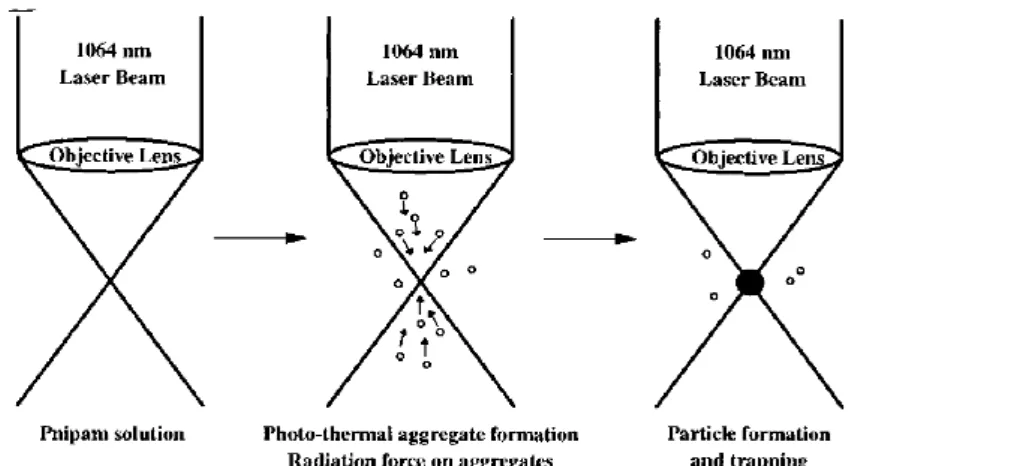
Recent works by Masuhara and his colleagues demonstrated that phase transition of PNIPAM can be induced not only thermally but also optically. In their photo-induced phase transition studies, they applied laser trapping in which a photon pressure induced by tight focusing of intense laser beam. Laser trapping induced phase transition was first demonstrated by Ishikawa et al. where a single PNIPAM microparticle formation/disappearance by turning on/off of a focused near infrared (NIR) laser beam under an optical microscope [32]. Induced phase transition is explained by local heating around the laser spot since H2O has an overtone absorption

band at NIR region. When the trapping laser was introduced into solution, the hydrogen bond between solvent and polymer will be corrupted by heating and then the polymer will become like a small single particle. Radiation force caused by focused laser beam will collect these particles and trapped particles are assembled and forming spherically-shaped microparticle at the focal spot as schematically depicted

Figure 0.2 Schematic drawing of PNIPAM phase transition. Coil state: Before phase transition Globule state: After phase transition

20

in Figure 0.3.

Figure 0.3 Focus laser beam induced molecular assembly formation of PNIPAM in aqueous solution. Figure from reference [33]

The following work was done by Hofkens et al. [34] who used D2O as solvent to

suppress the absorption of the overtone of O-H stretching band. D2O has less

absorption at 1064 nm and temperature elevation can be drastically suppressed; thus thermal phase transition is prevented under examined condition. Even using D2O as

solvent, they succeeded to induce microparticle formation due to the phase transition. It means that photon pressure induced by tight focusing of trapping laser light can collect molecule around the focal spot and form molecular assembly with non-contact, non-invasive and non-destructive manner with trapping and manipulation of molecules and molecular clusters. Thus, laser trapping technique is very good method for studying phase transition dynamics under photon pressure by combining

21

conventional optical microscopy such as bright field imaging, fluorescence imaging, fluorescence spectroscopy and lifetime imaging microscopy.

1.2 Laser trapping

Laser trapping is a very powerful technique which is widely applied in many research field, such physics, chemistry, biochemistry and biology. This tool is advantageous to manipulate micrometer particle freely without contact directly by focused intense laser light.

1.2.1

History of laser trapping

In early 1970s, Ashkin et al. demonstrated that optical forces could manipulate micron-sized dielectric particles in gas phase and liquid.[35] They identified two forces exerted to the object under photon pressure: a scattering force which work in the direction of the incident light beam and gradient force which pointing in the direction of the intensity gradient of laser beam.[36] This investigation led to the development of the single-beam gradient force optical trapping and was applied to wide range of objects from neutral atom to biological molecules. This unique technique has a revolutionary impact in broad area of science which mainly

22

discussing about single particle. In biology, it was used to study folding and unfolding of DNA, bacterial motion, and an activity of molecular motors.[37] Also in other area, an optical tweezers is a powerful tool especially for three dimensional manipulation of micrometer-particle. Masuhara et al. performed the experiments combining optical trapping with several microscopic techniques as fluorescence, absorption spectroscopy, photochemistry and electrochemistry.[38] Recently they have been applying this technique to induce a crystallization of biological molecules.[39]

By focusing a laser beam tightly with high numerical aperture (NA) objective lens, the dielectric particle will experience a force due to the momentum transfer from scattered photons as shown in Figure 0.4.[40-42] This trapping force can be decomposed in two components; (1) scattering force and (2) gradient force. The scattering force is in the direction same as light propagation, meanwhile the direction of gradient force is same as the direction of spatial light gradient. For the stable trapping, the axial gradient force should be larger than scattering force, then light can collect particles to the focal spot. This condition can be satisfied by using high NA objective lens which enables to make a diffraction limited spot size by sharp focusing of laser beam.

23

First, the particle radius (r) is larger than the trapping laser wavelength (), (r >> ). In this condition, it will be considered as Mie scattering regime and the optical forces exerted to the particle can be handled with ray optics (Figure 0.4). By Newton’s third law, the momentum change of incident photon is equal to the momentum change of particle and the direction is opposite. The force induced by momentum change is proportional to the light intensity. If the refractive index of spherical particle is larger than that of surrounding medium, the direction of the force matches to the direction of intensity gradient. Vise versa, if the refraction index of particle is smaller than that of medium, then the direction will be opposite. Thereofore, the first condition can trap the particle at the focal spot of the trapping laser and the second cannot.

Figure 0.4 Schematic diagram of ray optics for typical trapping which the refraction index of particle is larger than that of the medium. Redraw from [42].

24

Second, the particle is far smaller than the trapping laser wavelength (r << ) [40]. In this case particle can be treated as Rayleigh particle. We can treat the particle as point dipole for the calculation of working force to the particle. The force can be written as below; F=1 2aÑE 2+a ¶ ¶t(E´B)...1.1, a=4pe_bg3 (na/ nb) 2 -1 (na/ nb)2+2 ...1.2 .

Here, the E and B in equation 1.1 mean electric field and magnetic flux density, r means the radius of spherical particle which.  is polarizability. na and nb mean the

refraction index of particle and medium. The first and second terms of eq. 1.1 mean gradient and scattering force, respectively. When na > nb, the direction of gradient

force is in direction of light intensity. For a focused NIR laser beam, the gradient force is usually larger than the scattering force which leads a stable trapping of the particle at the focal spot.

1.3 Fluorescence microscopy/spectroscopy for phase transition

dynamics study

Steady-state and time-resolved fluorescence spectroscopy have been very powerful tool for molecular spectroscopic investigation of fluorescent molecules in

25

condensed phase. During a couple of decades it has grown dramatically due to the development of new optics, detectors, methods, and combing with different measurement systems such as microscopy, and we can detect very tiny signal from a single molecule. Fluorescence spectroscopy and time-resolve fluorescence measurement have already been very useful tool for the imaging of molecular dynamics in chemical, physical, and biological systems with single-molecule level. Fluorescence technique is used in so many applications, two-photon excited fluorescence (TPEF), fluorescence correlation spectroscopy (FCS) and so on. By introducing and combining with these techniques, fluorescence measurements can provide further information on a wide range of molecular process, such as intramolecular interaction, rotational diffusion, conformation changes, and binding interaction in biological systems, and also light induced phase transition dynamics.

We will construct fluorescence lifetime imaging microscopy system to investigate dynamics of phase transition of PNIPAM under laser trapping condition. More details will be discussed in latter section.

1.4 Aim of this study

As we mentioned before, phase transition of PNIPAM can be induced by trapping laser focusing in solution. In this study, we aim to clarify laser trapping induced phase

26

transition dynamics by using fluorescently labeled PNIPAM molecule, 3-(2-propenyl)-9-(4-N,N-dimethyl-aminophenyl-phenanthrene)-co-poly(N-isoproylac rylamide) (VDP-PNIPAM). As we mentioned above, the use of a fluorescent probe molecule is effective for studying the molecular motion of PNIPAM systems, as Winnik et al. have demonstrated in previous. We constructed fluorescence microscopy/spectroscopy system which is based on wide-field fluorescence and bright field microscope for the visualization of phase transition dynamics. We also constructed stage-scanning fluorescence lifetime imaging microscopy system to investigate photon pressure induced phase transition dynamics with more quantitative approach.

In addition to these phase transition dynamics study, we have found interesting novel phase transition behavior of PNIPAM derivatives. We found unusual two color laser induced phase transition under laser trapping; an introduction of weak UV light induces further phase transition. Although photon density of second UV laser is much weaker than that of trapping laser by 8 to 10 orders of magnitude, phase transition expansion when trapping laser power is higher than the threshold occurred very efficiently. We will also study phase transition dynamics of this unusual behavior and discuss from molecular spectroscopic view points.

27

2.

Experiment

2.1 Materials

Deionized water prepared with water purifier system (Sartorius, sarui611DI) and deutarated water (D2O, >99%) purchased from Sigma-Aldrich was filtrated with a

syringe filter (pore size; 0.22 mm, SLGV 013 SL, Millipore) before usage. Poly-(N-isopropylacrylamide) (PNIPAM, >99%, average molecular weight: 1.9 ~2.2 x104) was purchased from Sigma-Aldrich and used without further purification. Its structure is shown in Figure 2.1a.

For fluorescence microscopy and spectroscopy of one and two color laser induced phase transition, an intramolecular fluorescent probe, which is 3-(2-propenyl)-9-(4-N,N-dimethyl-aminophenyl-phenanthrene) (VDP), was used. Structure of VDP-PNIPAM is shown in Figure 2.1b. VDP-PNIPAM was prepared by radical polymerization as reported elsewhere.[43, 24, 26] Its molecular weight is about 3.0x104 which was determined by size exclusion chromatography. It contains 0.1 mol% of VDP unit: namely only one VDP unit is included in a single PNIPAM chain.

Sample solution was prepared by adding a solvent to powder polymer sample (PNIPAM and VDP-PNIPAM) and left for over night at room temperature to ensure that polymer was totally dissolved solution. A concentration of PNIPAM and

28

VDP-PNIPAM solution for trapping experiment was adjusted to 3.5 wt% both for H2O and D2O cases.

Steady state absorption and fluorescence spectra of the sample were measured by absorption spectrophotometer (V-670, Jasco) and fluorescence spectrophotometer (F-4500, HITACHI)

2.2 Bright field transmission imaging and fluorescence

imaging/spectroscopy system:

Laser trapping-induced phase transition behavior of PNIPAM and VDP-PNIPAM was observed by microscopy system which depicted in Figure 2.2a. The laser trapping

29

microscopy system used in this study is based on an inverted microscope (IX71, Olympus) equipped with double backport. We can introduce two different light sources easily to the microscope objective lens with this configuration. A near-infrared NIR laser beam of continuous wave (CW) Nd:YVO4 laser (Matrix

1064-10-CW, Coherent) at the wavelength of 1064 nm was used as a trapping light source. Trapping laser was focused into the sample solution in sealed glass chamber through an objective lens (40X, N.A.: 0.95). Trapping laser power was adjusted to 100 mW ~ 1.2 W at sample position by using variable neutral density filters. It should be noted that all the laser power mentioned in this study was measured value through objective lens.

Prepared PNIPAM and VDP-PNIPAM sample solutions were placed in a homemade sealed glass chamber which was made by sandwiching piled parafilm with two cover glasses (24 mm x 30 mm, 100 m thickness, Gold Seal) as shown in Figure 2.2b. The cover glass was cleaned by detergent and potassium hydroxide solution for several times prior to use for chamber fabrication. The thickness of the sample chamber was adjusted by piling parafilm where the average distance between two cover glasses is ~90 μm. Focusing position of the trapping laser was set to 10 μm lower than the bottom surface of upper cover slip; i.e. 80 μm from the bottom glass substrate surface.

30

Laser trapping-induced phase transition was recorded by bright field transmission imaging with using a halogen lamp as light source and CCD and EMCCD camera as for the detector.

We also performed wide-field fluorescence imaging of phase transition behavior. We used 325 nm line of CW He-Cd laser (IK-3401R-F, Kimmon) and, 405 nm CW diode laser (Cube 405-100C, Coherent) as for fluorescence excitation light source. In addition to these CW lasers, we also used second harmonic (SH) of femtosecond Ti:Sapphire laser (Tsunami, Spectra Physics) operated at 750 nm where we can obtain 375 nm second harmonic generation (SHG) output as for excitation light. This pulsed laser was also used in fluorescence lifetime experiments and more details are mentioned later. Excitation laser beams at 375 and 405 nm were introduced coaxially from the bottom of the sample thorough the same objective lens as well as trapping laser as depicted in Figure 2.2a. Fluorescence excitation laser beams were focused to the back imaging plane of objective lens to achieve collimated light after objective lens. Collimated light can irradiate more than ~150 μm observation field under microscope and it is sufficiently wide for our observation. In contrast, a 325 nm excitation light was introduced to the sample from the above without using objective lens since transmission efficiency of microscope objective at this wavelength is too low to obtain sufficient power density for wide-field fluorescence imaging. Beam spot

31

size of 325 nm is ~ 3 mm at the sample position. luorescence signal was detected by EMCCD camera (PhotonMAX, Princeton instruments).

Fluorescence signal was divided into two path by introducing beam splitter in the detection optical path as shown in Figure 2.2a. One of the light path was used for the spectrum measurement which passed through confocal pinhole placed in an optically conjugated plane of a focal plane of objective lens. Therefore we can detect the fluorescence signal merely from a focal spot. The light passed through the confocal pinhole was focused to the entrance slit of spectrograph (MS125, Oriel) equipped with cooled CCD (i-Dus DU401A-BR-DD, Andor) to obtain fluorescence spectra. By using this fluorescence microscopy/spectroscopy setup, we can examine simultaneous wide-field fluorescence imaging and confocal fluorescence spectroscopy of the molecules trapped under exerted photon pressure.

All the trapping experiments were carried out at room temperature (25˚C) and 50~60% of humidity condition.

32

2.3 Microscopy setup: Fluorescence lifetime imaging microscopy

system

Fluorescence lifetime of the molecules will give more useful information about molecular dynamics of laser trapping-induced phase transition. We have carried out Figure 2.2 (a) Schematic diagram of microscope setup for bright field transmission imaging and wide-field fluorescence imaging/spectroscopy. (b) A drawing of sealed glass chamber.

33

fluorescence lifetime observation of fluorescently labeled VDP-PNIPAM in addition to fluorescence imaging and spectroscopy. We used CW Nd:YVO4 laser (Millenia X,

Spectra Physics) pumper mode-locked femtosecond Ti:Sapphire laser (Tsunami, Spectra Physics) as excitation light source of fluorescence lifetime measurements. The output wavelength of this laser can be adjusted from 700 to 980 nm. To excite VDP moiety with SHG, operation wavelength was adjusted to 750 nm. Repetition rate, maximum output power and pulse width at 750 nm are 80MHz, 800 mW and ~150 fs. Fundamental output from Ti:S oscillator was introduced to a pulse selector (Model 3980, Spectra Physics) in which an acousto-opitc modulator (AOM) thinned out pulses from the pulse train to change the repetition rate.

We took a SHG by focusing fundamental after passing pulse picker and obtained 375 nm excitation light. A SHG of Ti:S laser was introduced into the objective lens coaxially with NIR trapping laser to excite the molecules from the different back port of the microscope as depicted in Figure 2.3. Emission from the sample was corrected by the same objective lens and brought to an optical fiber which is connected to a single photon counting avalanche photo diode (APD) (SPAD, Micro Photon Device) after passing the confocal pinhole. Thus, obtained fluorescence lifetime is basically from the confocal volume and can obtain with high spatial resolution. Fluorescence signal passed a set of filters to eliminate unwanted scattering light from excitation

34

laser light, environment and sample prior to introduce to the APD. The fluorescence emission collected by the APD was coupled into an in-house assembled time-correlated single photon counting system to construct the lifetime decay histogram. Data collection was controlled by PicoHarp 300 TCSPC system (PicoQuant). Detailed diagram of TCSPC system is shown in Figure 2.4. In short, converted signal of emission was sent from APD to signal router (PHR 800, PicoQuant). Signal router transfers the APD signal as decay signal to photon counting module. A reference signal to construct fluorescence decay histogram, an oscillating laser signal detected by fast photodiode (818-bb-21, Newport) was brought to the photon counting module, and used to construct by calculating the difference of arrival timing as we explained about a principles of TCSPC in a previous section. Instrument response function (IRF) was generated by collecting scattered laser light from a colloidal scattering solution (Ludox CL-X colloidal silica 45 wt% suspension in water, Sigma-Aldrich ). Lifetimes were measured at the emission wavelength of VDP and in each case data were collected until 10,000 counts in the channel of maximum intensity. Then, fluorescence lifetimes were extracted from the measured decay curves using FluoFit (PicoQuant) which implements nonlinear least-squares error minimization analysis, based on the Simplex and Lavenberg-Marquardt algorithms. The final quoted result was determined by the fit, which had a  value of less than 2.0 and

35

residual trace that was symmetric about zero.

As shown in Figure 2.3 constructed fluorescence lifetime measurement system is integrated with fluorescence imaging/spectroscopy system. Therefore we can perform simultaneous fluorescence lifetime measurement, fluorescence imaging and spectroscopy. It is quite advantageous to study the phenomena that occur with hierarchic dimension such as phase transition.

Figure 2.3 Schematic diagram of fluorescence lifetime imaging microscopy system.

36

Figure 2.4 System of fluorescence measurement: (a) A picture of TCSPC system and (b) cabling diagram.

37

3.

Phase transition of PNIPAM induced by trapping laser

As we described in a previous section, we can induced phase transition of PNIPAM by focusing trapping laser. Temperature elevation will cause macroscopic phase transition of PNIPAM solution, meanwhile focused trapping laser beam induces microparticle formation at the focal spot due to the phase transitions. We will use non-labeled PNIPAM to find suitable experimental conditions for phase transition dynamics study of fluorescently labeled PNIPAM.

3.1 Laser trapping-induce phase transition of PNIPAM

Local phase transition induced by focused NIR laser beam can be considered in two reasons, thermal effect of NIR laser by the vibronic absorption of solvent and photon pressure. To clarify these two effects, we prepare the sample with D2O

solution to suppress the absorption of NIR laser.

The results of laser induced phase transition in H2O and D2O at the same trapping

laser power (725 mW) were shown in Fig. 3.1. In both solution conditions, we could observe particle formation depend on applied laser power and it disappeared by terminating trapping laser irradiation as well as previous report.[33] However, obtained results showed drastic different in both phase transition particle size and particle formation time depending upon the solvent even though trapping laser power

38

was the same.

The particle formed in H2O solution was larger than that formed in D2O under

same laser power as shown in Figure 3.1. Average diameter of the particle formed in H2O (~14 m) at 725 mW of trapping laser power was almost twice of that formed in

D2O as mentioned in Table 3.1. Particle size became larger with increasing the laser

power more than the size of view field size of EMCCD under microscope (more than 60 m) in H2O. In contrast, maximum size saturated around 10 m in D2O. Formed

particle size became obviously lager in H2O when the laser power was higher than

600 mW as shown in Figure 3.2.

Particle formation time, which is defined as a necessary time to generate a microparticle due to phase transition, was also clearly different between H2O and D2O.

Particle formation time became shorter with increasing the laser power as shown in 錯誤! 找不到參照來源。. Particle was formed almost immediately after starting irradiation more than 600 mW laser power in H2O, meanwhile it needed about 10 min

at the same laser power in D2O (Table 3.1).

We restricted the observation time for 30 min to determine power threshold of phase transition. We observe quite rapid phase transition even at 200 mW in H2O, but

PNIPAM in D2O could not show phase transition less than 425 mW within 30 min.

39

size and NA of used objective lens (NA=0.9) to be ~50 MW/cm-2. Therefore we can define phase transition threshold power density in D2O is ~50 MW/cm-2. On the other

hand, threshold power density in H2O can be said less than 25 MW/cm-2 under

examined condition.

Figure 3.1 Local phase transition induced by laser trapping in (a) ~ (d) H2O and (e)

~ (f) D2O. Laser power was 725 mW. Scale bar = 10 μm. Time indicated in the

40

Figure 3.3 Phase transition time change upon laser power. The symbols show PNIPAM in H2O (▲) and D2O (■) and VDP-PNIPAM in H2O (◆)

and D2O (★), respectively.

Figure 3.2 Trapping laser power dependent formed particle size difference. The symbols show PNIPAM in H2O (▲) and D2O (■) and VDP-PNIPAM in

41

Different solvent shows obvious difference on particle size, particle formation time and threshold power density of phase transition. In H2O solution, the trapping

power threshold to observe phase transition is lower than that in D2O solution. The

phase transition time is also shorter than that in D2O solution. At the same trapping

power, the particle is larger than that in D2O solution. It is interpreted due to a

generated heat in H2O is more than that in D2O. The heat caused by the vibronic

absorption at NIR region in H2O solution is larger than in D2O solution.

Ito et al. reported that 1 W of 1064 nm laser focusing to H2O and D2O induces

about 22 and 2.6˚C temperature elevation, respectively.[44] The temperature elevation in D2O solution is quite small compare with in H2O solution. Therefore phase

transition in H2O occurred more efficiently.

In contrast to in H2O solution, temperature elevation is almost 1/10 in D2O. All

the experiments were done at room temperature (~25˚C) and solution temperature cannot reach LCST (~32˚C), even we focus 1 W of trapping laser. However we Table 3.1 Phase transition time and particle size in H2O and D2O solution.

Power (mW) 225 425 525 625 725 1000 1300 Time (s) H2O 148.0 116.0 26.5 0.0 0.0 NA**1 NA**1 D2O NA**2 1000.0 898.0 529.0 283.0 60.0 45.0 Size ( m) H2O 3.3 5.3 5.5 11.6 14.1 NA**1 NA**1 D2O NA**2 5.5 6.4 6.7 6.8 9.5 9.1

42

experimentally observed microparticle formation due to the phase transition. As well as the observation in previous case, phase transition in D2O suggests molecular

assembly formation of PNIPAM due to not only temperature elevation but exerted photon pressure. However we should avoid ambiguity of undesirable heat generation during laser focusing to the solution.

3.2 Heating effect of glass substrate

We are interested in the molecular assembling and phase transition which induced by photon pressure. Therefore it should be better to suppress temperature elevation and/or generation during trapping laser irradiation. It is suggested that NIR laser absorption by glass substrate will generate a heat and elevate temperature.[44]

To clarify temperature elevation due to trapping laser absorption by substrate, we examined glass and quartz which does not absorb NIR light and compared by observing phase transition behavior. Laser focus point was fixed to 10 m bellow of upper substrate of the chamber.

Figure 3.4 shows the formed phase transition microparticle both glass and quartz sample chamber. PNIPAM/H2O solution was used and laser power was higher than

525 mW. In both substrates, particle size became larger with increasing the laser power. As we can see in Figure 3.5a, the particle size formed in each sample chamber,

43

glass substrate cases showed larger particle in all examined laser power range. It implies that glass substrate generate more heat than quartz due to the absorption of trapping NIR laser light.

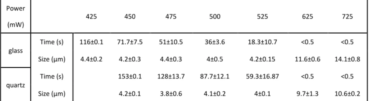
Although phase transition times were almost similar both glass and quartz substrate above 600 mW, it shows slight difference at 525 mW (Figure 3.5b). More detailed examination of power dependency between 450 to 525 mW range (Figure 3.6) showed clearly longer phase transition time for quartz substrate.

As well as in H2O, glass substrate showed faster phase transition, larger particle

size, and additionally, lower power threshold of phase transition in case of D2O

solution as seen in Figs. 3.7a and 3.7b. Threshold of phase transition with glass substrate, 0.7 W, was much lower than that for quartz substrate at 1.1 W.

The values of phase transition time and particle size on glass and quartz substrates induced in H2O and D2O are summarized in Table 3.2 and 3.3, respectively.

44

Figure 3.5 Power dependence of (a) particle size and (b) phase transition time in H2O solution. The symbols show glass (▲) and quartz (●).

Figure 3.4 Phase transition-induced microparticle formation in H2O with

(a) ~ (c) glass substrate and (d) ~ (f) quartz substrate at each trapping power.

45

Figure 3.7 Power dependence of (a) phase transition time and (b) particle size formed in the glass (■) and quartz (◆) chamber. PNIPAM/D2O solution was used.

Figure 3.6 Power dependence of phase transition time in H2O solution with

46

3.3 Position dependence of PNIPAM phase transition

Consider with the heating effect of substrate, we need to compare the phase transition behavior at different height in the chamber. When trapping laser was focused at the middle of the chamber where is far away from the substrate and will have less heating effect from the substrate. We also check the position dependence with glass and quartz substrate. PNIPAM/H2O solution was used. Laser powers at 450

and 550 mW for glass and quartz substrate were used, respectively. Trapping laser power was decided to form similar size of microparticle in both substrate cases. Results of position dependence experiment for different substrate are summarized in

Table 3.2 The PNIPAM phase transition time and size at each trapping laser power in H2O solution Power (mW) 425 450 475 500 525 625 725 glass Time (s) 116±0.1 71.7±7.5 51±10.5 36±3.6 18.3±10.7 <0.5 <0.5 Size (μm) 4.4±0.2 4.2±0.3 4.4±0.3 4±0.5 4.2±0.15 11.6±0.6 14.1±0.8 quartz Time (s) 153±0.1 128±13.7 87.7±12.1 59.3±16.87 <0.5 <0.5 Size (μm) 4.2±0.1 3.8±0.6 4.1±0.2 4±0.1 9.7±1.3 10.6±0.2

Table 3.3 The PNIPAM phase transition time and size at each trapping laser power in D2O solution

Power (mW) 725 925 1100 1200 1300 1400 1500 glass Time (s) 283.0±45.3 283.5±20.5 311.7±133.3 139.3±60.5 172.5±27.8 33.5±12 Size (μm) 6.1±1.1 4.8±0.3 7.7±2.5 7.9±3.4 8.8±2.1 33.7±1.3 quartz Time (s) 335.0±67.4 258.3±104.6 176.0±63.6 94.0±57.5 Size (μm) 5.1±0.8 6.6±0.3 5.6±1.3 9.1±2.4

47

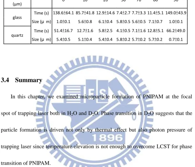
Figure 3.8. The values of phase transition time and particle size at the different focusing position in the sample chamber for glass and quartz are summarized in Table 3.4, respectively. When the focusing position is far from the substrate more than 10 μm, we can see stable microparticle formation with similar particle size and less size fluctuation. This tendency is more obvious in quartz substrate case. It suggests that the heating effect due to NIR absorption by substrate can be suppressed by using quartz as substrate. Hereafter, we use quartz instead of glass for chamber fabrication aiming to achieve and observe more stable phase transition behavior.

Figure 3.8 Position dependence of (a) phase transition time and (b) particle size with glass substrate(■), and (c) phase transition time and (d) particle size with quartz (▲) substrate. PNIPAM/H2O solution was used. Trapping laser powers

48

3.4 Summary

In this chapter, we examined microparticle formation of PNIPAM at the focal spot of trapping laser both in H2O and D2O. Phase transition in D2O suggests that the

particle formation is driven not only by thermal effect but also photon pressure of trapping laser since temperature elevation is not enough to overcome LCST for phase transition of PNIPAM.

We also discussed about the heating effect due to trapping laser absorption by solvent and substrate. The heating effect from the substrate can be identified by changing the substrate from glass to quartz which do not absorb NIR light. The quartz substrate showed higher trapping power threshold and longer phase transition time compared with glass substrate case. This clearly indicates that we can suppress temperature elevation and heating effect by using quartz as substrate. Position

Table 3.4 Phase transition time and size at different position of the sample chamber. Position (μm) 0 10 20 50 70 80 90 glass Time (s) 138.6±64.1 85.7±41.8 12.9±14.6 7.4±2.7 7.7±3.3 11.4±5.1 149.0±43.9 Size (μ m) 1.0±0.1 5.6±0.8 6.1±0.4 5.8±0.5 5.6±0.5 7.1±0.7 1.0±0.1 quartz Time (s) 51.4±16.7 12.7±1.6 5.8±2.5 4.1±0.5 7.1±1.6 12.8±5.1 66.2±49.0 Size (μ m) 5.4±0.5 5.1±0.4 5.4±0.4 5.8±0.2 5.7±0.2 5.7±0.2 0.7±0.1

49

dependence of phase transition implies when the trapping position is far more than 10 m from the substrate, we can induce rather stable phase transition without particle size fluctuation. Hereafter, we will use quartz as substrate to prevent heating effect of the substrate.

50

4.

Fluorescence lifetime measurement and construction of

fluorescence lifetime imaging microscopy (FLIM) system

Steady-state and time-resolved fluorescence spectroscopy have been powerful tool for molecular spectroscopic investigation of fluorescent molecules in condensed phase. During a couple of decades it has grown dramatically due to the development of new optics, detectors, methods, and combing with different measurement systems such as microscopy, and we can detect very tiny signal from a single molecule. Fluorescence spectroscopy and time-resolve fluorescence measurement have already been very useful tool for the imaging of molecular dynamics in chemical, physical, and biological systems with a sensitivity at single-molecule level. Fluorescence technique is used in so many applications: two-photon excited fluorescence (TPEF), fluorescence correlation spectroscopy (FCS) and so on. By introducing and combining with these techniques, fluorescence measurements can provide further information on a wide range of molecular process, such as intramolecular interaction, rotational diffusion, conformation changes, and binding interaction in biological systems.

51

4.1 Fluorescence from molecule.

There are two very important characters of fluorophore, lifetime and quantum yield. Figure 4.1 shows Jablonski diagram which explains photo-induced activation/deactivation pathways after an excitation of fluorescent molecules. Fluorescence quantum yield and lifetime can be explained along with the rate constants indicated in Figure 4.1. Fluorescence quantum yield is defined by the percentage of emitting photons relative to absorbed photons as explained with eq. 4.1,

where kr, kic, kisc are radiative rate constant, rate constant of internal conversion and intersystem crossing, respectively.

52

Based on above diagram, the rate equation of fluorescence from S1 state is explained with eq. 4.2;

By taking an integration of eq. 4.2, we obtain eq. 4.3

The (S1)0 means the concentration of S1 state at the initial condition, as it to say

instantly after photo excitation. Because emission light intensity is proportional to the concentration of the molecules in S1 state, it can be presented by following equations,

Figure 4.1 Jablonski diagram. S0 and S1 are ground and lowest excited singlet state,

respectively. T1 is lowest excited triplet state. The k means rate constant for ka:

absorption; kr: fluorescence kr’: phosphorescence, knr, knr’: non-radiative

deactivation,kisc : intersystem crossing

53

Usually, is called lifetime of S1.

The lifetime means the average time of fluorophore remains in the excited state after the excitation. Lifetime is sensitive to the interaction between fluorophore and its environment, thus we can obtain environmental information not only from spectral change but also lifetime change.

4.2 Time-correlated single photon counting

For measuring lifetime of fluorescent molecules, there are two typical methods; time domain and frequency domain method. Here we will introduce only time domain method since we use this method for lifetime measurement in this study. For time domain measurement, problems are (1) it is hard to obtain data with ordinary electronic transient recorders and (2) fluorescence signal is usually too weak to make a decay curve. The most popular approach to solve the problem is using “Time-Correlated Single Photon Counting” (TCSPC) method. Equation 4.4 depicts how we can obtain the lifetime of fluorophore by mathematical calculation based on the transitions in Jablonski diagram. By taking the log of integration of eq. 4.2 we

54

obtain following equation (for single exponential decay)

The lifetime can be found as a slope of decay curve. For multi-exponential decay, the intensity of fluorescence can be written as eq. 4.7 by introducing additional decay components,

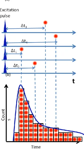
Figure 4.2a shows schematic drawing how emitted photon from excited molecule will be tagged to construct fluorescence decay curve. Here we decide signal arriving time of excitation light as time t=0. As shown in Figure 4.2a observing timing of emitted photon from excited fluorophore vary depending upon excitation event. Therefore we can record photon observing time as a function of the difference between excitation light arriving time and fluorescence photon arriving time as depicted in the figure such as t1, t2, … . Intensity decay with delay time after the

excitation pulse laser coming can be constructed by taking a histogram of arriving photons which becomes as the blue line in Figure 4.2b which can be described as eq. 4.7. From the intensity decay curve, we can calculate lifetime of sample. TCSPC method is base on the highly repetitive single photon counting. As shown in Figure 4.2, photon will be tagged at the time depending upon the delay (i.e. the difference of

55

the arrival time between excitation pulse and emitted photon from the molecule) after excitation pulse coming. With TCSPC method, it will count just the first photon coming after excitation pulse. Then the time of photon coming will be store in a phton counting module with time-correlated histogram. By using high repetition rate pulse laser as excitation light source, this graph can be taken efficiently by doing this process repeatedly in a short time. The typical result is a histogram with an exponential decay towards later times as shown in Figure 4.2b (lower panel).

56

This method requires that we need to restrict the photon number to be less than one for each cycle to guarantee that the histogram of photon arrivals would obtained from a single shot time-resolved analog recording. Because the detector and electronics have a dead time, if plural number of photons in one excitation are emitted,

Figure 4.2 Principle of TCSPC. (a) Variation of an arriving time of emitted photon from fluorophore and (b) a histogram constructed from the photons came after the excitation pulse. This histogram is fluorescence decay curve.

(a)

57

the system would very frequently register the first photon and then missing the following ones: this is called as pulse pile-up. To avoid this problem, the average counts rate at detector should be at most 1~5% of the excitation photon rate. For example, if the excitation laser pulse repetition rate is 80MHz, the average detector count rate should not exceed 4MHz. However, we need to consider the high count rate to make decay histogram quickly, especially for dynamics of lifetime change and fast molecule transition studies. When planning the experiment, we should consider these points and try to find the optimized condition.

Combining the decay curve with eqs. 4.6 and 4.7, we can obtain lifetime information of the molecule. For measuring decay time of intensity, we need specialized electronics to measure the time delay between excitation and emission. The electronics setup is as shown in Figure 4.3. The synchronous signal come from excitation light source is brought to a time-to-amplitude converter (TAC), which generate voltage signal that increases linearly with time, to be the start point to calculate time delay. The detection signal will be sent to a constant function discriminator (CFD), which will accurately calculate the arriving time of pulse, and then its signal is sent to TAC to be stop signal. From the voltage of TAC, we can determine the delay time between excitation pulse and emission from the molecule. Then the voltage information will be converted to digital signal by an