國立臺灣大學理學院大氣科學所 碩士論文
Department of Atmospheric Sciences College of Science
National Taiwan University Master Thesis
以區域標記法進行閃電放電過程之模擬
Simulation of Lightning Discharge with Region-Labeling Method
曾敏端 Min-Duan Tzeng
指導教授:陳正平 博士 Advisor:Jen-Ping Chen, Ph.D.
中華民國 107 年 7 月
July, 2018
摘要
本研究利用天氣研究與預報模式(WRF)輔以大氣電學模組探討強降水與活躍
閃電現象的關係。WRF 中的電學模組對於放電過程僅以基本圓柱狀結構描述,不
能有效區分雲對地與雲內閃電放電過程。本研究改進放電通路的設定方式,以區
域標記法對高電場區域進行連通,容許複雜幾何通路的放電計算,並且區分雲對
地與雲內閃電,進一步對於不同放電特性進行計算。模擬結果顯示新方案能有效
改進閃電放電頻率過高的現象,且閃電極性與雷暴雲微物理過程之間具有強烈關
聯性:雲對地正閃電好發於軟雹初生的對流前期,雲內閃電好發於具有較強上升氣
流的對流成熟期,雲對地負閃電則伴隨層狀區降水發生於對流消散期。以上閃電
與對流結構發展的關聯性有助於強降水事件的即時預警。
關鍵字: 區域標記法、WRF 模式、閃電模擬、非感應電荷分離機制、總體參數法
ABSTRACT
This study investigated the relationship between intense precipitation and vigorous
lightning flashes using the Weather Research and Forecasting model coupled with an
atmospheric electricity module WRF_ELEC. The WRF_ELEC module can describe
basic discharging process, but it cannot identify intra-cloud and cloud-to-ground flashes.
This study improved the discharging algorithm of WRF_ELEC by applying the
region-labeling method, which provides more detailed information on the electrical
properties and geometry of lightning flashes. Simulation results show that the proposed
method can significantly improve the lightning flash frequency. Also, it is able to reveal
the polarity of lighting flash associated with the microphysical structure of thunderstorm.
Positive cloud-to-ground flash is active at initial stage of thunderstorm when graupel
formation becomes significant. Intra-cloud flash is active at the mature stage of
thunderstorm when the updraft is strong enough to reach high levels. Negative
cloud-to-ground flash is active during the dissipating stage of thunderstorm when
precipitation results mainly from the outflow stratiform region. These important
indicators are valuable for the nowcasting of heavy precipitation.
Keywords: Region-labeling method, WRF model, lightning simulation, non-inductive
charge separation mechanism, bulk parameterization
Table of Contents
1. Introduction ... 1
2. Methodology ... 5
2.1 Charging/Discharging Physics... 5
2.2 Region-Labeling Method ... 10
2.3 Total Lightning Location System (TLDS) ... 10
2.4 Model setup ... 11
3. Results ... 13
3.1 Simulated convective system ... 13
3.2 Flash Frequency ... 14
3.3 Microphysics Structure ... 15
3.4 Charges in Hydrometeor ... 17
3.5 Polarity of Flash ... 19
3.6 Effective Channel Radii ... 20
4. Summary and Future Work ... 21
References ... 25
Figrues ... 29
Table ... 44
Appendix ... 45
Index of Figures
Figure 2-1: A three-dimensional view of the discharge using the Cy method (a, c) and the RL method (b, d). Upper panels show the region with significant positive charges (orange) and negative charges (blue); the discharge regions are indicated with green-shading areas. Lower panels are charge distribution after flash. ... 29 Figure 2-2: The charge attached on graupel per-collision with ice/snow particle. The
values below -40℃ are invalid and are filtered out during model iteration.
Mansell et al. (2005) ... 30 Figure 2-3: Schematic of the basic charge distribution in the convective region of
thunderstorm. (Stolzenburg et al. 1998) ... 30 Figure 2-4: The critical electric field for diagnosis of initial points of lightning. This is a
demonstration of isothermal atmosphere with 293K. ... 31 Figure 2-5: A demonstration of RL method labels an individual channel. Blue grid is the
initial grid with electric field magnitude greater than Einit. Gray grids are the grids with electric field greater than τEinit, which is the potential to join the channel. Red grids are grids which have been checked by RL method. Green grids are contiguous grids that join the channel. The algorithm terminates while all of the grids in the channel have been checked by RL method. ... 32 Figure 2-6: Domain configuration of the WRF model. Black block region is the nested
second domain with 4 km grid spacing. Red block is the nested third domain with 4/3 km grid spacing. ... 33 Figure 2-7: Synoptic weather chart at initial time of simulation, 1800 UTC, May 24th,
2008 ... 33 Figure 3-1: Frequency of independent cloud series lifetime. ... 34 Figure 3-2: Evolution of the main cloud series. Each dot is a contiguous cloud segment.
Colors denote the volume ratio of upward motion of each cloud segment. ... 34 Figure 3-3: Time series of IC (a) and CG (b) frequency, and flashes overlapped with
domain-averaged precipitation (c). The total number of flashes through the entire simulation is noted at legend. Note that Cy only simulate total flashes which makes no difference between IC and CG. The scales of RL and observed flashes are shown on the left axis, whereas that of Cy is shown on the right axis.
The time axis of observation is shifted and labeled at the upper axis. ... 35 Figure 3-4: Evolution of the vertical profile of hydrometeor contents in one of the
largest thunderstorm cell. The cell is determined by 0.1 g/kg condensed phase water contiguous region with similar RL approach. QI: cloud ice; QS: snow;
QG: graupel; QC: cloud drop; QR: rain drop ... 36
contents. ... 37 Figure 3-6: Similar to Figure 3-4, excepts it shows the cumulative positive charge
attached on hydrometeors. ... 38 Figure 3-7: Similar to Figure 3-4, excepts it shows the cumulative negative charge
attached on hydrometeors. ... 39 Figure 3-8: Similar to Figure 3-4, excepts it shows the average space charge density.
Top: customized colorbar for positive charges; bottom: customized colorbar for negative charges. ... 40 Figure 3-9: Proportion of charges carried by hydrometeors in three types of flashes. Left panels (a, c, e) are the limiting reagent of lighting: positive charges for PCG (a), negative charges for NCG (c) and minor charges for IC (e). Right panels (b, d, f) are opposite-sign charges. Horizontal axis is the electric quantity of the limiting reagent which determines the magnitude of neutralization. ... 41 Figure 3-10: Frequency of effective channel radii under different insulating factor
scenario. ... 42 Figure 3-11: Relation between effective channel radii and quantity of electric charge
inside channel. Shading denotes the CG counts. Contour denotes the IC counts with values of 1, 10, 100, 1000. ... 43
Index of Table
Table 1: Notable option of the WRF model as used used this study. ... 44
1. Introduction
Lightning occurs extensively in severe weather and can inflict casualties and
economic loss. The victims struck by lightning have 10-30% death rate, and most of the
survivors suffered from permanently disabled body functions (Ritenour et al. 2008).
Lightning flash also creates electromagnetic pulses which can disrupt or damage
electronic components. The mechanism of lightning and the relationship between
flashes and heavy precipitation have interested researchers for decades. From the aspect
of long-term climatology, lightning plays an important role on the formation of NOx and
O3, which are important troposphere greenhouse gases, during summertime (Zhang et.
al. 2003). In addition, the polarized ice crystals that orientate along the electric field
affect the albedo of anvil significantly. From the aspect of weather forecast and nowcast,
the thunderclouds with more flashes indicate that their ice phase process is more active,
subsequently producing heavier precipitation and, in extreme cases, resulting in
destructive hailstones. On the microscopic scale, charged hydrometeors may have
higher accretion rate and retain large sizes without breakup during collision. Therefore,
understanding the formation of lighting in thunderstorm is valuable for risk assessment
and for studying feedbacks of atmospheric electricity.
Lightning discharge is a rapid adjustment process that releases the instability in
atmospheric electrical field. This process is difficult to simulate with weather models
(e.g. the Weather Research and Forecasting (WRF) model) due to the extraordinary
scale variation of discharging channels. The width of lighting channel (around an inch)
is much smaller than the grid size (0.5~30 km) of weather system models. On the other
hand, the length of lightning branches can stretch over numerous grids; therefore,
cross-grid communication is essential for lightning scheme. As such, current numerical
algorithm of discharge scheme depends on the spatial and temporal scale of the model.
Moreover, the time step used in the mesoscale model is much larger than that of the
lightning flash, so the whole cycle of discharge needs to be resolved instantaneously.
Lightning simulation methods can be divided roughly into two approaches: explicit
channels flash and bulk flash. One example of explicit channels flash is the dielectric
breakdown model (Niemeyer et al. 1984, Wiesmann and Zeller 1986, Mansell et al.
2002), which is originally applied to the breakdown process of plastics or gases. This
sort of model simulates step-by-step propagation of channel extension and branching.
Branching, bonding or extension of channel relates to the ambient electric field as a
probability function for any new segment that joins the channels. Each propagation step
iterates the electric potential to make sure that the channels are equipotential. The
simulation results are similar to the dielectric breakdown experiments. The channels
tend to propagate and branch in the region of larger charge density. However, the scale
of dielectric breakdown models is much smaller than typical time steps and thus not
practical to be use in the WRF model.
The bulk lightning scheme reduces the sophistication of lightning structure by using
simple channel shapes. The parameterization in Helsdon et al. (1992) is a simple rod
that traces the environmental electric field bi-directionally, and can only perform
inter-cloud or intra-cloud (IC) channeling. The branching phenomenon is suppressed
because of the geometry limitation. MacGorman et al. (2001) presented a revised
lightning parameterization with a dumbbell shape to simulate the branched region with
high charge density at both ends of bidirectional channels. Since the space charge is
usually lifted in the air, cloud-to-ground (CG) channels are diagnosed from the channel
with low base. To simplify the lightning process and adapt to the WRF model, Fierro et
al. (2013) parameterized the channels using a cylindrical-shape discharging zone around
the initiation points. The channels stretch from ground to the top of model, such that all
channels are CG channels. In contrast to previous bulk lightning schemes, this study
incorporated the region-labeling (RL) method, which was commonly used in image
processing and also applied in convective cell analysis (Tsai and Wu 2017), to allow for
more flexible geometry of lightning discharging regions, and also to differentiate
between IC and polarized CG.
The main objectives of this study are to better understand how the geometry of
discharging channel affects the lightning flashes properties, and to investigate the
possibility of nowcasting heavy precipitation using lightning signal.
2. Methodology
This study used the three-dimensional compressible nonhydrostatic WRF model
(version 3.7.1) with Advanced Research WRF dynamic solver (WRF-ARW; Skamarock
et al. 2008). The initial and atmospheric electricity variables are derived by additional
physics module WRF_ELEC (Fierro et al. 2013) that is specifically incorporated into
the National Severe Storms Laboratory (NSSL) two-moment four-ice microphysics
scheme, which applies the charging physics from Mansell et al. (2005). The main
improvement in this study is the identification of lightning discharge channels. Basic
lightning discharge channel in WRF_ELEC assumes cylindrical geometry centered at
lightning initiation points. The proposed discharging method adapts the RL algorithm
(Tsai and Wu 2017) for both IC and CG identifications with flexible shapes related to
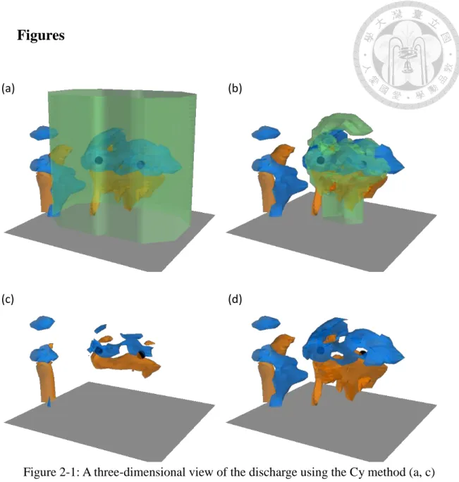
ambient electric field. The geometry difference of the above method is illustrated in Fig.
2-1. A thunderstorm case in 2008 over northern Taiwan is selected for model simulation.
2.1 Charging/Discharging Physics
2.1.1 Charging mechanism
A series of laboratory experiments (Takahashi 1978, Gardiner et al. 1985, Jayaratne
et al. 1983, Ziegler et al. 1991, Brooks et al. 1997, Saunders and Peck 1998) suggested
that non-inductive charge separation from riming graupel colliding with other solid
hydrometers plays a big role in thunderstorm electric field construction. Laboratory
experiments generally agreed that the charges attached on graupel by non-inductive
charge separation are positive sign under high temperature and high riming accretion
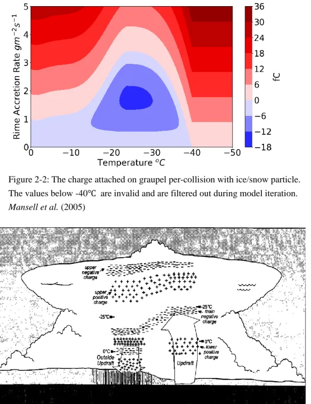
rate (RAR) as illustrated in Fig. 2-2. This study calculates the non-inductive charge for
grid cell with the following equation (Mansell et al. 2005):
δ𝑞 = 𝐵𝐷𝐼𝑎(𝑉𝑔− 𝑉𝐼)𝑏𝑞(𝑅𝐴𝑅) (1)
where B, a, b are coefficients depending on crystal size (cf. Table 1 in Mansell et al.
2005); subscript g and I represent graupel and the other ice-phase hydrometeor; D is the
mean volume diameter; V is mass-weighted terminal fall speeds; q(RAR) is charge
separation factor given by Mansell et al. (2005):
𝑞+(𝑅𝐴𝑅) = 6.74(𝑅𝐴𝑅 − 𝑅𝐴𝑅𝑐) (2a)
for positive charging (𝑅𝐴𝑅 > 𝑅𝐴𝑅𝑐),
𝑞+(𝑅𝐴𝑅) = 3.9(𝑅𝐴𝑅𝑐− 0.1) × (4 [𝑅𝐴𝑅−(𝑅𝐴𝑅(𝑅𝐴𝑅 𝑐−0.1)/2
𝑐−0.1) ]2− 1) (2b) for negative charging (0.1gm−2s−1< 𝑅𝐴𝑅 < 𝑅𝐴𝑅𝑐).
The critical RAR (𝑅𝐴𝑅𝑐) is given by Eqs. (21-23) in Mansell et al. (2005):
𝑅𝐴𝑅𝑐(T) = {𝑠(𝑇):
𝑘(𝑇):
0 ∶
𝑇 > −23.7℃
−23.7℃ > 𝑇 > −40℃
𝑇 ≤ −40℃
(3)
𝑠(𝑇) = 1 + 7.9262 × 10⁻²𝑇 + 4.4847 × 10⁻²𝑇2+ 7.4754 × 10⁻³𝑇3
+5.4686 × 10⁻⁴𝑇4+ 1.6737 × 10⁻⁵𝑇5+ 1.7613 × 10⁻⁷𝑇6 (4a)
𝑘(𝑇) = 3.4 [1 − (−23.7+40|𝑇+23.7|)3] (4b)
However, the 𝑅𝐴𝑅𝑐 for the charging-sign reverse is still uncertain because it is difficult
to control the surface property of mixture hydrometeors in cloud chamber (Saunders
2008). The charge separation may come from the mass transfer of quasi-liquid layers of
hydrometeors (Baker et al. 1994). Because of the polarity of water, an overall
electrically neutral hydrometeor tends to be negative at the surface and positive in its
core. The negative charges at the surface transfer to another hydrometeor following the
mass flow of quasi-liquid layers when collision happens. Mass flow direction depends
on the thickness difference of quasi-liquid layers between hydrometeors. Hydrometeors
with warmer surface or higher growth rate have thicker quasi-liquid layers, and may
lose its mass when collision happens. Therefore, one hydrometeor, which has thicker
quasi-liquid layer, is positively charged after collision, and the other one is negatively
charged. Prior studies (Krehbiel 1986, Stolzenburg et al. 1998) show that there are two
mainly charged region at middle and upper level of thunderstorms. The middle one is
negatively charge and the other is positively charged (Fig. 2-3). There are thin charged
layers of opposite sign at the boundary of cloud base (positive) and cloud top (negative),
which are the inductive charges caused by main charged region.
2.1.2 Discharging Mechanism
The original WRF_ELEC uses a cylindrical volume with prescribed radius
(typically 12 km) around the initial points to redistribute spatial charges (hereinafter
called the Cy method). The initial points are the grids with electric field magnitude
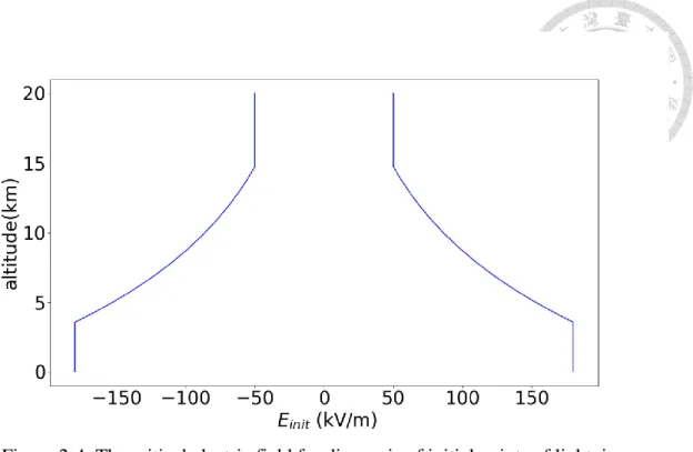
greater than an altitude-dependent threshold, 𝐸𝑖𝑛𝑖𝑡, defined as follows:
𝐸𝑖𝑛𝑖𝑡 = 2.84 × 10²(𝑘𝑉𝑚)𝜌𝜌
0 (5)
𝐸𝑖𝑛𝑖𝑡 ∈ (50,180)𝑘𝑉 𝑚
where 𝜌 is the density of air and 𝜌0=1.225 kg/m3 is a constant. Values of 𝐸𝑖𝑛𝑖𝑡from
the above equation is illustrated in Fig. 2-4. The channel size of the Cy method is
specific and does not depend on the ambient electric field. All spatial charges inside the
volume participate in the discharge. Neutralization of charges depends on the total
amount of charges (positive or negative) inside the channel and the charge density.
Charge density structure is conserved inside the channel but with a smaller magnitude
because of the neutralization of charges. However, there is no difference between the
neutralization of charges of IC and CG flashes.
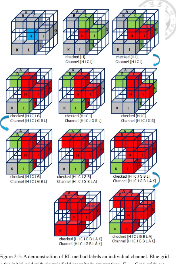
This study modified the discharge module by determining the channel with RL
method (details given in the next section). The RL method connects adjacent regions
with significant electric field. The critical electric field is set to be a portion of 𝐸𝑖𝑛𝑖𝑡
using an insulating factor, 𝜏. Grids with electrical field magnitudes greater than 𝜏𝐸𝑖𝑛𝑖𝑡
can then join the lightning flash channels. This method automatically changes the
geometry of channel according to the ambient electric field. IC and CG are identified
through the altitude of channel base. IC channels occur in the air, such that the net
charge in the atmosphere is conserved during the neutralization process. CG channels
connect to the ground and direct the atmospheric charges to the Earth, so the charge is
not conserved in the air. The equations of charge neutralization are expressed as
follows:
𝑃𝐶𝐺 ∶ 𝑑𝑞 = {−𝛾𝑞 𝑞 > 0
−𝛾𝑞𝑁𝑃 𝑞 < 0 (6a)
𝑁𝐶𝐺 ∶ 𝑑𝑞 = {−𝛾𝑞𝑁𝑃 𝑞 > 0
−𝛾𝑞 𝑞 < 0 (6b)
𝐼𝐶: 𝑑𝑞 = 𝛾(𝑞̅ − 𝑞) (6c)
where PCG and NCG indicate positive and negative CG, respectively; 𝑞 is the charge
density and 𝑑𝑞 is the change in charge density due to neutralization; 𝑞̅ is the average
charge density in the channel; N and P are total negative and positive charges in the
channel, respectively; and 𝛾 is a prescribed coefficient to control the magnitude of
neutralization. Magnitude of grounding current in CG depends on the major sign charge
in the channel. On the other hand, neutralization of charge in IC is limited by the minor
sign charge in the channel. Charges remaining from neutralization are redistributed
according to the charge density before discharge. To compare with the Cy method, the
effective radius of channel is defined as follows:
𝑅𝑐ℎ = √𝜋𝐷𝑉𝑐ℎ
𝑐ℎ (7)
where 𝑅, V, D are radius, volume and depth of channel, respectively.
2.2 Region-Labeling Method
The region-labeling (RL) method (also called connected-component labeling or blob
extraction) is an algorithm commonly used in computer visualization (Ballard and
Brown 1982) and has also been applied in cloud object analysis (Heiblum et al. 2016;
Tsai and Wu 2017). The algorithm detects contiguous region with a key property above
a prescribe threshold, as demonstrated in Fig. 2-5. In this study, the concerned property
is the electric field magnitude. The RL method is also applied to track convective cells
in this study (with the concerned property of cloud condensate amount). The temporal
tracking targets a series of convective cells by the overlapping region in the continuous
time interval, which is 2 minutes in this study.
2.3 Total Lightning Location System (TLDS)
The lightning data used in this study were from the Total Lightning Location System
(TLDS) measurements provided by the Taiwan Power Company. The TLDS is an array
of antenna that detects and ranges lightning by measuring the arrival time of LF/HF
radiation from CG flashes at multiple stations. For IC events, TLDS measures the
interferometry of VHF radiation and reports the two-dimensional location of flashes
projected on the ground. The system is more sensitive to IC than to CG events because
of the limitation of frequency band.
The TLDS divides the lightning impulses into six categories indexed from 0 to 5.
Category 0 is singleton IC signal; 1 is the initial signal for continuous IC; 2 is the
transitional signal of continuous IC; 3 is the termination of continuous IC; 4 is CG
signal; 5 is returning stroke of CG. The simulated lightning is compared with category 0
for IC and category 4 for CG, and the polarity of CG is determined by the sign of peak
current.
2.4 Model setup
The domain configuration and some notable options selected in WRF model are
shown in Fig. 2-6 and Table 1. The model runs with Cy lightning discharge method and
the RL method mechanism are designated as the control and experiment runs,
respectively. The insulating factor 𝜏 is set to 0.2 for the main simulation. The
sensitivity of 𝜏 is evaluated by virtual lightning discharge, and does not affect the
electricity of main simulation, with 𝜏 ranged from 0.2 to 0.8.
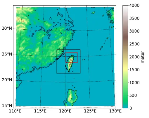
Figure 2-7 shows the synoptic weather chart at the initial time of simulation, which
is 18:00 UTC, May 24th, 2008. The unstable weather condition before the mei-yu front
arrival is favorited for thunderstorm activities. The convection system in the simulation
is quasi-stationary at the offshore region and over the terrain. The rationale behind the
case selection is that RL method is a serial algorithm that cannot afford a large domain
for fast convective system propagation.
3. Results
3.1 Simulated convective system
Appendix A1 shows the composite reflectivity from the Central Weather Bureau
(CWB) radars and simulated by model from 06:00 to 22:00 LST, May 25th, 2008. Note
that the simulated electricity does not feedback to the microphysics or environmental
properties, therefore both RL and Cy methods have identical precipitation and storm
microphysical structures. There are two major convective systems in the simulation. The
earlier convective system was initiated at an offshore region, and is weaker than the
later one. The convective system simulated is somewhat stronger than observed, and is
more aggregated which exhibited a more linear structure. The later convective system
was initiated over land and propagated westward to merge with the dissipating offshore
convective system. By looking at the composite radar reflectivity and time series of
lightning flashes, it is found that the simulated systems lead the observed systems. So,
the simulated results are shifted forward by 3 hours in the comparison analyses.
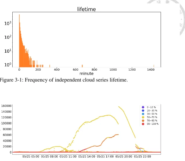
With output rate of every two minutes, there are 121044 cloud segments being
labeled in this one-day simulation. Among the 121044 cloud segments, there are 7073
cloud series with their life-time distribution shown in Fig. 3-1. The lightning flashes are
produced by only one of the cloud series, which is the major series with 77504
segments including those being merged or split up. This series contains two major
convective systems, one offshore and the other over the terrain. The evolution of size
and the ratio of updraft (speed > 0 m s-1) volumes are shown in Fig. 3-2. The offshore
convection was initiated at 06:20 LST and diminished after 10:30 LST. The convective
system over terrain was initiated as chaotic convective cells from 09:20 to 11:40 LST
and then organized into a large convective system. A significant merger event seemed to
happen at 19:00; however, it is actually a merger between two dissipating anvil, which
marked the decline of the convection system that contrasts with the organization of the
chaotic convections. The following discussion of microphysical and electrical properties
is focused on this major cloud series.
3.2 Flash Frequency
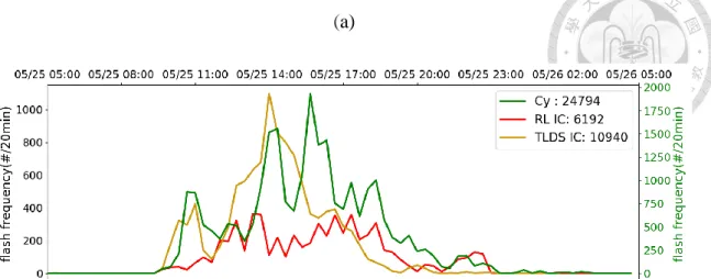
The simulated frequencies of IC (Fig. 3-3a) and CG (Fig. 3-3b) flashes are of a
similar magnitude as observed, except during the peak hours of 13:00 to 15:00 LST
when the model underestimates IC and overestimates CG counts. However, the total
flash counts are similar. These biases are caused by the low 𝜏 value that used which
tends to connect channel to ground. Thus, the CG channels release more energy than
usual and suppress the IC channels. In comparison, the Cy method generally
overestimates the total flash counts by a factor of two.
Figure 3-3c shows that PCG peak occurred at the early stage of thunderstorm
activity, and it leads the precipitation peak by about an hour, which is different from the
results of Tai et al. (2017), who found that IC peak leads precipitation. IC flashes
developed following PCG during the mature stage of thunderstorm but without a
significant peak. NCG developed even later, with two major peaks occurred during the
dissipation stage of thunderstorm. After the second NCG peak, the precipitation
terminated as the storms die out.
The PCG flashes concentrated at the updraft region while the IC flashes are around
the edges of the updraft region (Appendix A2). On the other hand, the NCG flashes
distributed sporadically at the outflow stratiform region of the convection (Appendix
A3). The polarity of RL CG is opposite to the TLDS observed. The uncertainty of
lightning polarity and the relationship between precipitation and flashes will be
discussed in Section 3.3 and 3.4.
3.3 Microphysics Structure
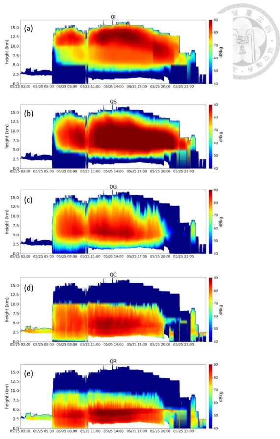
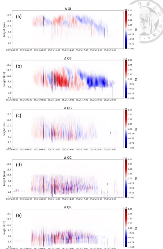
Figure 3-4 shows the water content (mixing ratio) and tendency (Fig. 3-5) of each
hydrometeor category (QC: cloud drop; QR: raindrop: QI: cloud ice; QS: snow; and QG
graupel) in the main cloud system. The earlier convection offshore produces less
precipitation than the subsequent convection over terrain that developed after 09:20 LST.
At the initial stage of both convections, particles in cloud are mainly cloud drops (Fig.
3-4d) and cloud ice (Fig. 3-4a). Raindrops (Fig. 3-4e) developed below the melting
level, indicating that they should be originated from graupel (Fig. 3-4c) or snow (Fig.
3-4b) melting. Significant riming for graupel formation happened at 06:00 LST, which
is also the time for the first (but minor) PCG peak. Explosive formation of graupel
happened around 11:00 LST when the second and major peak of PCG occurred. The
upward-tilting-with-time pattern in cloud drops (Fig. 3-5d) and cloud ice (Fig. 3-5a)
suggests that these two hydrometeors form at the lifting region. In contrast, some
downward propagating patterns happen in raindrops (Fig. 3-5e) and snow (Fig. 3-5b)
because these two hydrometeors grow by accreting other hydrometeors while falling.
The high variability of cloud drops tendency indicates that cloud drops form in the
convective region with significant updraft and downdraft. On the other hand, cloud ice
tendency is smoother than that of cloud drop because it mainly forms at the stratiform
region of cloud. The patterns of convective and stratiform regions can also be found in
the tendency of raindrops and snow, respectively. The graupel tendency (Fig. 3-5c) has
no significant vertical-propagation pattern, because the tendency of graupel depends on
the cloud drop concentration and the rimed ice/graupel particle size. The concentration
of cloud drop is greater at lower levels, but the rimed particles are somewhat higher
levels. Thus, the tendency of graupel is vertically invariant.
3.4 Charges in Hydrometeor
Figures 3-6 and 3-7 show the charges carried by graupel, cloud ice, snow and rain
drops. Graupel particles that collide with ice particles tend to carry positive charges at
low (warmer) altitudes (Fig. 3-6a) and negative charges at high(cooler) altitudes (Fig.
3-7a), as the process depends on the ambient temperature and riming rate (Fig. 2-2). Ice
particles that collide with riming graupel at lower levels carry negative charges to the
higher levels and reach to the top of thunderstorm. These negatively charged ice
particles aggregate with each other and form snow particles, which combine the
negative charges from the colliding particles (Fig. 3-7b). On the other hand, ice particles
that collide with riming graupel at higher levels tend to carry positive charge. These
positively charged ice particles can aggregate and form positively charged snow
particles (Fig. 3-6b) at the middle level.
PCG peak revealed significant riming process at low levels. Graupel particles grew
explosively by riming process and produced plenty of positively charged graupel
particles that fall toward the cloud base. The concentrated charges at the cloud base
induced significant PCG flash events before heavy precipitation arrived at the ground.
Unceasing IC indicates that the updraft is strong enough to produce large snow particles
which carried negative charges. The negatively charged snow particles fall to lower
levels and neutralized the air containing positively charged graupel particles.
NCG peak is the signal of termination of electrification at low levels. The negatively
charged particles fall to cloud base without any positively charged particles to be
neutralized. Therefore, negative charges released to the ground form NCG flashes. NCG
flashes also occurred in the outflow stratiform region of convective cloud, therefore the
electrification at low level is weak.
Figure 3-8 shows the space charge density in the cloud. The thunderstorm is overall
negatively charged. These are the remaining charges from the active PCG. Although the
size of lower positive region seems to be large as shown in Appendix A3, the charge
density is much less than the negative charge at middle level (Fig. 3-8). The top
positively charged region is also insignificant and somewhat overwhelmed by negative
charges. The graupel particle at low altitude carries more positive charges than
conventional knowledge, and ice particle carrying negative charge also contrasts with
prior studies (Krehbiel 1986, Stolzenburg et al. 1998). According to the conventional
knowledge of thunderstorm with triple-pole structure (main negative, upper and lower
positive charged region; Fig. 2-3), the riming accretion rate in thunderstorm should
lower than 1 gm-2s-1 (Fig. 2-2), as such the main charge region at lower level is
negatively charged and the upper level is positively charged. These results indicate that
the charging mechanism (Fig. 2-2) in the model may have some bias or the simulated
riming rates are unrealistically large, which lead to positive charging of graupel at low
level. If an additional description of electric polarization of dielectric hydrometeors is
added into the model, this could reduce the instability of electrical field. At the same
time, it would induce opposite charge layers at the boundaries of the main charged
regions. These layers would reduce the cloud-to-ground flashes at cloud base and
trigger the transient luminous events at cloud top. Although this research focused on the
discharging process, it is nonetheless important to re-examine the charging mechanism
and the effects of dielectric property of hydrometeors in the future.
3.5 Polarity of Flash
Figure 3-9 shows the proportion of positive and negative charges carried by
hydrometeors in three types of flashes (i.e., PCG, NCG and IC). As indicated by Eq. (6),
the limiting reagent of charge neutralization is the positive charges, negative charges
and minor sign charges for PCG, NCG and IC, respectively. The results here agree with
the hypothesis discussed in the previous section. The most important electrified
hydrometeor is graupel, which carried about 80% of positive charges in PCG (Fig. 3-9a).
For the negative-charge-major IC (positive part of Fig. 3-9e), graupel particles also
carry 80% of positive charges in the channel. These two types of flash are the most
frequent flashes in simulated thunderstorms. For NCG at the dissipating stage of storm
activity, 50% of negative charges are on cloud ice while 40% are on snow. This strongly
suggests that PCG and IC are indicators for the intense formation of low level graupel
particles which is a prerequisite for heavy precipitation formation.
3.6 Effective Channel Radii
Figure 3-10 shows the frequency of effective channel radii (Eq. 7) throughout the
entire simulation. The mode of radian increases when 𝜏 decreases. With lower 𝜏, the
conductivity of atmosphere is higher ,which is advantageous for channels to spread out
and connect with adjacent channels. The results suggest that the radian of 12 km for Cy
method flash channels is too large in most of the cases. Most of the radian of channels is
around 3 km. Only few IC and NCG channels are greater than 10km. Cy method
overdamps the charge density in weak flashes and underestimates the magnitude of
extreme cases. Fig. 3-11 shows that the channel of RL method is able to select an
adequate region to neutralize charges. The magnitude of flashes will not saturate even in
extreme cases.
4. Summary and Future Work
This study developed a cross-grid communicating discharging process. This is
essential for lightning discharging process, but the numerical algorithm is incompatible
to the current electricity scheme in the WRF model. It takes lots of effort to break the
barrier of the grids in different parallel calculating components. With the flexibility of
lightning channel geometry, both IC and CG flashes are differentiable using the
proposed RL method. The RL method can also label the identical channels in different
grid spacing theoretically. This is an added value of the RL discharging method.
A key contribution of this study is a clearer realization of the features of
3-dimensional charge distribution that determine the discharge of lightning. With the RL
method, lightning channels adapt to an adequate geometry for involving the charged
hydrometers. Instead of the thin-tube channel that branches at two ends (MacGorman et
al. 2001), the discharging channel is more like a prolate or a dumbbell (Fig. 2-1). Like
typical bulk lightning discharge, the detailed structure of lightning channel cannot be
resolved within the WRF model. Charges remain in thin-tube channel is negligible in
kilometer-scale grid sizes.
In comparison to the original WRF_ELEC with Cy discharge, the RL method
provides more realistic descriptions of the discharge processes, including polarity of CG
and charge conservation of IC. The number of flashes reduced by 35% while the
neutralization is weaker in IC flashes as compared with the Cy method. The lightning
flashes are charge sinks that release the instability of electric field. The RL method only
neutralizes charges over unstable region, which is more efficient to reduce the instability
than the Cy method. The unrealistic perturbation that would appear using the
WRF_ELEC scheme can be avoided by the channel selection strategy.
The sensitivity of 𝜏 suggests that the prescribed radian of 12km in Cy method
overestimates the size of channel and neutralizes the charges unrealistically. Unrealistic
perturbation other than unstable region in Cy method can be minimized through the RL
method. However, the prescribed 𝜏 in recent model is a preliminary assumption. The
real breakdown channel is determined by the conductivity of atmosphere, which is more
complex than the single factor 𝜏.
The polarity information from the RL method reveals the relationship between
lightning and microphysical features of thunderstorm. PCG flash peak indicates the
initial conversion of graupel at low levels. IC flash indicates that the updraft is more
than enough to produce large-size ice-phase particles at high levels. NCG flash peak
occurs while the thunderstorm is decaying. Updraft in decaying thunderstorm cannot
provide enough cloud drops for riming process. Then, negatively charged graupel
particles fall to cloud base and induce NCG flashes. These specific events are valuable
for nowcasting and are important sign for heavy precipitation. However, the polarity of
CG observed by TLDS is opposite with the RL simulated. TLDS detects the NCG peaks
at initial stage and PCG at dissipating stage, and the IC peaks is much stronger than the
RL method simulated. The RL simulated IC/CG ratio is 1:2.but the TLDS detected 3:1.
As it is difficult to configure the insulating factor due to the uncertainty of atmospheric
conductivity, there exists inconsistency between observed and modelled IC/CG ratio.
However, the ability to differentiate between IC and CG contributes much to our
understanding of the relationship between lightning and convection. By adapting IC/CG
ratio as standard for regulating lightning module, discharge process can be calibrated
more systematically. We look forward to simulate more weather system and perform
sensitivity test on conductivity parameterization. Although the simulated sign of
changes do not match with observed lightning, the experience of this study is valuable
for the simulation of lightning with sophisticated geometry. By re-examine the charging
mechanisms and provide more comprehensive physics description, simulations may be
more comparable with observation and suitable for lightening forecast in the future.
Future work may include feedback effects on hydrometeors caused by electric fields,
for example, electrophoretic force that enhances the collision efficiency of
hydrometeors or changes in sedimentation speed. More case studies for other types of
thunderstorm convection are also desirable for gaining a broader sense of the
electrification processes. The convection current in different types of convective
systems is an important boundary condition for ideal simulation of lightning channel
(Pasko et al. 1996) and thus is also worth paying attention in the future. Intensive
observation, such as balloon-carried electric field meter, can also be arranged to provide
more real-world verifications of model simulations.
References
Ballard, D. H., & Brown, C. M. (1982). Computer vision. Englewood Cliffs, NJ:
Prentice-Hall.
Brooks, I., Saunders, C., Mitzeva, R., & Peck, S. (1997). The effect on thunderstorm charging of the rate of rime accretion by graupel. Atmos. Res.,43(3), 277-295.
Fierro, A. O., Mansell, E. R., Macgorman, D. R., & Ziegler, C. L. (2013). The
Implementation of an Explicit Charging and Discharge Lightning Scheme within the WRF-ARW Model: Benchmark Simulations of a Continental Squall Line, a Tropical Cyclone, and a Winter Storm. Mon. Wea. Rev.,141(7), 2390-2415.
Gardiner, B., Lamb, D., Pitter, R. L., Hallett, J., & Saunders, C. P. (1985).
Measurements of initial potential gradient and particle charges in a Montana summer thunderstorm. J. Geophys. Res.,90(D4), 6079.
Heiblum, R. H., Altaratz, O., Koren, I., Feingold, G., Kostinski, A. B., Khain, A. P., ... &
Yaish, R. (2016). Characterization of cumulus cloud fields using trajectories in the
center of gravity versus water mass phase space: 2. Aerosol effects on warm
convective clouds. Journal of Geophysical Research: Atmospheres, 121(11),
6356-6373.
Helsdon, J. H., Wu, G., & Farley, R. D. (1992). An intracloud lightning parameterization scheme for a storm electrification model. J. Geophys. Res. Atmos., 97(D5),
5865-5884.
Jayaratne, E., Saunders, C., & Hallett, J. (1983). Laboratory studies of the charging of soft-hail during ice crystal interactions. Q. J. Roy. Meteor. Soc.,109(461), 609-630.
Krehbiel, P. R. (1986). The electrical structure of thunderstorms. The Earth’s electrical
environment, 90-113.
Macgorman, D. R., Straka, J. M., & Ziegler, C. L. (2001). A Lightning Parameterization for Numerical Cloud Models. J. Appl. Meteorol.,40(3), 459-478.
Mansell, E. R., Macgorman, D. R., Ziegler, C. L., & Straka, J. M. (2002). Simulated three-dimensional branched lightning in a numerical thunderstorm model. J. Geophys.
Res. Atmos.,107(D9).
Mansell, E. R., MacGorman, D. R., Ziegler, C. L., & Straka, J. M. (2005). Charge structure and lightning sensitivity in a simulated multicell thunderstorm. J. Geophys.
Res. Atmos., 110(D12).
Niemeyer, L., Pietronero, L., & Wiesmann, H. J. (1984). Fractal dimension of dielectric breakdown. Phys. Rev. Lett., 52(12), 1033.
Pasko, V. P., Inan, U. S., & Bell, T. F. (1996). Sprites as luminous columns of ionization produced by quasi-electrostatic thundercloud fields. Geophys. Res. Lett., 23(6),
649-652.
Ritenour, A. E., Morton, M. J., McManus, J. G., Barillo, D. J., & Cancio, L. C. (2008).
Lightning injury: a review. Burns, 34(5), 585-594.
Saunders, C. P., & Peck, S. L. (1998). Laboratory studies of the influence of the rime accretion rate on charge transfer during crystal/graupel collisions. J. Geophys. Res.
Atmos.,103(D12), 13949-13956.
Saunders, C. P. (2008). Charge separation mechanisms in clouds. In Planetary Atmospheric Electricity (pp. 335-353). Springer, New York, NY.
Skamarock, W. C., Klemp, J. B., Dudhia, J., Gill, D. O., Barker, D. M., Duda, M. G., ...
& Powers, J. G. (2008). A Description of the Advanced Research WRF Version 3.
Stolzenburg, M., W. D. Rust, and T. C. Marshall (1998), Electrical structure in
thunderstorm convective regions: 3. Synthesis, J. Geophys. Res., 103(D12), 14097–
14108.
Tai, J. H., Wang, Y. M., Yang, M. J. & Lin, P. H. (2017) The preliminary study of
applying intra-cloud lightning data to convective rain fall nowcasting. 大氣科學,
45(1),43-56。
Takahashi, T. (1978). Riming electrification as a charge generation mechanism in thunderstorms. J. Atoms. Sci., 35(8), 1536-1548.
Tsai, W., & Wu, C. (2017). The environment of aggregated deep convection. J. Adv.
Model. Earth Sy.,9(5), 2061-2078.
Wiesmann, H. J., & Zeller, H. R. (1986). A fractal model of dielectric breakdown and
prebreakdown in solid dielectrics. J. Appl. Phys., 60(5), 1770-1773.
Zhang, R., Tie, X., & Bond, D. W. (2003). Impacts of anthropogenic and natural NOx sources over the U.S. on tropospheric chemistry. P. Natl. Acad. Sci. U.S.A., 100(4), 1505-1509
Ziegler, C. L., Macgorman, D. R., Dye, J. E., & Ray, P. S. (1991). A model evaluation of noninductive graupel-ice charging in the early electrification of a mountain
thunderstorm. J. Geophys. Res.,96(D7), 12833.
Figures
Figure 2-1: A three-dimensional view of the discharge using the Cy method (a, c) and the RL method (b, d). Upper panels show the region with significant positive charges (orange) and negative charges (blue); the discharge regions are indicated with green-shading areas. Lower panels are charge distribution after flash.
(a) (b)
(d) (c)
Figure 2-2: The charge attached on graupel per-collision with ice/snow particle.
The values below -40℃ are invalid and are filtered out during model iteration.
Mansell et al. (2005)
Figure 2-3: Schematic of the basic charge distribution in the convective region of thunderstorm. (Stolzenburg et al. 1998)
Figure 2-4: The critical electric field for diagnosis of initial points of lightning.
This is a demonstration of isothermal atmosphere with 293K.
Figure 2-5: A demonstration of RL method labels an individual channel. Blue grid is the initial grid with electric field magnitude greater than 𝐸𝑖𝑛𝑖𝑡. Gray grids are the grids with electric field greater than 𝜏𝐸𝑖𝑛𝑖𝑡, which is the potential to join the channel. Red grids are grids which have been checked by RL method. Green grids are contiguous grids that join the channel. The algorithm terminates while all of the
Figure 2-6: Domain configuration of the WRF model. Black block region is the nested second domain with 4 km grid spacing. Red block is the nested third domain with 4/3 km grid spacing.
Figure 2-7: Synoptic weather chart at initial time of simulation, 1800 UTC, May 24th, 2008
Figure 3-1: Frequency of independent cloud series lifetime.
Figure 3-2: Evolution of the main cloud series. Each dot is a contiguous cloud segment. Colors denote the volume ratio of upward motion of each cloud segment.
(a)
(b)
(c)
Figure 3-3: Time series of IC (a) and CG (b) frequency, and flashes overlapped with domain-averaged precipitation (c). The total number of flashes through the entire simulation is noted at legend. Note that Cy only simulate total flashes which makes no difference between IC and CG. The scales of RL and observed flashes are shown on the left axis, whereas that of Cy is shown on the right axis. The time axis of observation is shifted and labeled at the upper axis.
Figure 3-4: Evolution of the vertical profile of hydrometeor contents in one of the largest thunderstorm cell. The cell is determined by 0.1 g/kg condensed phase water contiguous region with similar RL approach. QI: cloud ice; QS: snow; QG:
graupel; QC: cloud drop; QR: rain drop (a)
(b)
(c)
(d)
(e)
Figure 3-5: Similar to Figure 3-4, excepts it shows the tendency of hydrometeor contents.
(a)
(b)
(c)
(d)
(e)
Figure 3-6: Similar to Figure 3-4, excepts it shows the cumulative positive charge (a)
(b)
(c)
(d)
Figure 3-7: Similar to Figure 3-4, excepts it shows the cumulative negative charge attached on hydrometeors.
(a)
(b)
(c)
(d)
Figure 3-8: Similar to Figure 3-4, excepts it shows the average space charge density. Top: customized colorbar for positive charges; bottom: customized colorbar for negative charges.
Figure 3-9: Proportion of charges carried by hydrometeors in three types of flashes.
Left panels (a, c, e) are the limiting reagent of lighting: positive charges for PCG (a), negative charges for NCG (c) and minor charges for IC (e). Right panels (b, d, f) are opposite-sign charges. Horizontal axis is the electric quantity of the limiting reagent which determines the magnitude of neutralization.
(e) (c)
(a) (b)
(d)
(f)
Figure 3-10: Frequency of effective channel radii under different insulating factor
Figure 3-11: Relation between effective channel radii and quantity of electric charge inside channel. Shading denotes the CG counts. Contour denotes the IC counts with values of 1, 10, 100, 1000.
Table
Table 1: Notable option of the WRF model as used this study.
Simulation Period
20080524 18Z ~ 20080525 18Z (24 hrs) Domains setting
Domain 1 180 ×180 (12 km) 30s Domain 2 130 × 130 (4 km) 10s Domain 3 196 × 160 (1.33 km) 3.33s Vertical 50 layers; Ptop = 10 hPa Physics Options
Cumulus Kain-Fritsch (D1 only)
PBL YSU
SW radiation New Goddard LW radiation New Goddard Surface layer MM5 similarity
Land surface 5-layer thermal diffusion Microphysics NSSL 2-moment 4-ice scheme
(steady background CCN)
Appendix
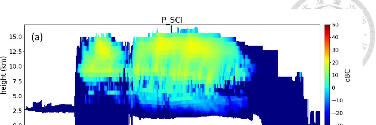
Appendix A1: Composite reflectivity and three-dimensional view of the convective cells.
Figure A1: Composite reflectivity and three-dimensional view of convection cell. Left panel: simulated hydrometeors with mixing ratio of 0.5g/kg. Blue: graupel; Salmon: cloud drop; Green: rain drop; Red: cloud ice; Violet: snow; Brown: hail. Middle panel:
simulated S-band (10cm) composite reflectivity. Right panel: composite reflectivity by the Central Weather Bureau radar system.
Appendix A2: Spatial distribution of Simulated and Observed Flashes.
Figure A2: Spatial distribution of Flashes. Left panel: simulated flashes by Cy method.
Middle panel: simulated IC by RL method; Right Panel: observed IC by TLDS.
Appendix A3: Spatial distribution of simulated CG and three-dimensional view of space charges.
Figure A3: Spatial distribution of simulated CG and three-dimensional view of space charge. Left panel: simulated space charge with concentration of 0.1nC/m3. Blue:
negative charges; Red: positive charges. Middle panel: simulated positive CG by RL method. Right panel: simulated negative CG by RL method.