應用安全存貨及備援廠商管理供應鏈斷鏈風險

國立臺灣大學管理學院商學研究所 碩士論文

Graduate Institute of MBA College of Management

National Taiwan University Master Thesis

應用安全存貨及備援廠商管理供應鏈斷鏈風險

Investigation of Solutions for Safety Stock and Backup Supplier Selection for Supply Chain

Disruption Risk Management

劉沛玟 Liu, Pei-Wen

指導教授: 許鉅秉 博士

Advisor: Sheu, Jiuh-Biing Ph.D.

中華民國 104 年 6 月

June, 2015

I

II

誌 謝

研究所的生活一轉眼就到了要結束的時候了，在寫這篇畢業論文的時候，總 是會不斷的回想著過去學生生涯的種種一切。雖然過去也是一名管理學院的學生，

但對於供應鏈領域可以說是完全的陌生，也從未想到自己可以有機會完成這個學 位以及這篇論文。雖然自己也付出了一些努力，但這一路上有太多的人幫助我、

提攜我，要感謝的人實在是數都數不盡，因此在這篇論文的一開始，想要先向這 些幫助過我的人，獻上我最高的謝意。

首先是我的指導老師－許鉅秉教授，老師是物流管理界的大師，但卻願意花 其寶貴的時間指導碩士論文，真的是非常感謝老師。每次若有問題想要請教老師，

老師總是不厭其煩的撥空指導我，再加上老師幽默風趣，因此每次找完老師後不 僅問題得到了解答，連心情也會好上許多。真的很感謝老師這一年半來的指導與 照顧，老師不僅教導我專業領域的知識，更教導我做人處事的道理，使我終身受 益。此外，老師更熱心給與我未來繼續就學的建議，真的是位非常替學生著想的 老師。在此，特別向許老師獻上我的感謝之意。

再來是感謝台大商研所的同學們，台大商研所是全國數一數二的企研所，這 裡聚集著最優秀的同學們，每當自己想要偷懶或者放鬆時，看到同學們的努力總 會讓我不忘時時督促自己。能在這樣的班上學習，實屬本人的榮幸。

最後是我的家人，家人從小就給我好的環境讀書，讓我衣食不虞匱乏，我能 有今天的一點點成就，可以說完全歸功於我的家庭。他們總是無私的照顧我、包 容我，讓我勇往直前追求我的夢想。在這裡我要對他們說，謝謝你們、我愛你們。

還有太多的人需要一一感謝了，但礙於篇幅這裡僅僅列一些對我而言最重要 的人，但我也一併在此向過往幫助過我的人說一聲，非常感謝您。

III

摘 要

隨著科技與運輸工具的進步，供應鏈越來越全球化，但也越來越脆弱及易受 影響。因此，在當今社會，關於供應鏈風險管理的議題也就越來越重要。當一家 公司的供應鏈系統易受其環境影響而變得相當脆弱時，公司的決策者就必須考慮 採取減輕策略來因應大環境的衝擊。在本研究中，本文採取了兩種預防性的減輕 策略來避免供應鏈系統受到中斷風險嚴重地影響。本文分析了安全存貨及備援廠 商兩種減輕策略的特性，接著再將此兩種減輕策略應用在一起以達到最低的運用 減輕策略成本為目標。

本文模型主要探討在兩級的供應鏈系統下，當零售商是以採取持續檢視政策 及受到隨機需求，並且其補貨來源基本上是來自於一家有可能會遇到中斷危機的 主要供應商的情境下所做的討論。在上述的情況下，本研究找出了同時採取此兩 種預防性減輕策略並且能夠達到最低目標成本的最適解。通過本研究，可以了解 能夠達到最低目標成本的安全存貨與備援廠商的最適分配比例為何。此外，本研 究也進行了敏感度分析及情境分析，讓決策者能了解在不同情境下所應採取的行 動及分配減輕策略的比例。數值分析的結果證明了本文模型的正確性，並且也提 供決策者一個可靠的決策依據，讓其可以在確保最低成本的條件下採取本文模型 所建議的減輕策略比例。

關鍵字：供應鏈中斷風險，減輕策略，安全存貨，備援廠商，隨機存貨管理

IV

ABSTRACT

With improvement in technology and transportation, supply chain becomes more international and, unfortunately, more vulnerable. Hence, issues about supply chain risk management are more and more important nowadays. When company’s supply chain is very vulnerable to its environment, company’s decision maker should consider applying mitigation strategies to survive in this environment. In our research, this study applies two proactive mitigation strategies to prevent our supply chain system from serious disruption risk. This study analyzes the characteristics of safety stock and backup supplier and applies these two mitigation strategies together to achieve the lowest cost of adopting mitigation approaches.

Our model considers stochastic demands with continuous-review system under two-echelon supply chain in which a retailer replenishes its inventory basically from a vulnerable primary supplier who may have a big chance to encounter disruptions.

Under this circumstance, this study find out the optimal solution of proactively adopting two mitigation strategies together so as to achieve our objective function, the lowest working inventory cost. This study understands the optimal adopting proportions of backup supplier and additional safety stock that can let us achieve our lowest cost. These studies also do sensitivity analyses and scenario analyses to understand what decision maker should do when under different situations. The results of numerical analysis prove that our model is valid and can really help decision maker to make proper decisions while does not have to worry about drastic changes on total cost.

Keyword: Supply chain disruption risk, Mitigation strategy, Safety stock, Backup

supplier, Stochastic inventory management

V

CONTENTS

誌 謝 ... II 摘 要 ... III ABSTRACT ... IV

Chapter 1 Introduction ... 1

1.1 General Background Information ... 1

1.2 Research Purpose ... 4

1.3 Research Scope and Limitation ... 5

1.4 Research Framework and Process ... 6

Chapter 2 Literature Review ... 9

2.1 Supply Chain Risk and Management ... 9

2.2 Supply Chain Disruption Risk ... 13

2.3 Safety stock ... 16

2.4 Backup supplier ... 19

Chapter 3 Combination of Mitigation Methods ... 23

3.1 Problem Definition, Research Method and Purpose ... 23

3.2 Basic Assumptions ... 26

3.3 Model Development ... 28

Chapter 4 Numerical Analysis ... 42

4.1 Numerical Example ... 45

4.2 Verification of the Model ... 48

4.3 Sensitivity Analysis... 50

4.4 Scenario Analysis ... 60

4.5 Chapter Summarization ... 64

Chapter 5 Conclusions ... 66

5.1 Conclusion ... 66

5.2 Prospect ... 68

Reference ... 70

VI

LIST OF FIGURES

Figure 1.1 Global NAND flash memory revenue market share by quarter………..….2

Figure 1.2 Framework of this research………..8

Figure 3.1 Regular situation of two-echelon supply chain network……….30

Figure 3.2 Disruptive situation of two-echelon supply chain network………30

Figure 3.3 Inventory policy at the retailer with cycle length ^𝑄 𝜇………...32

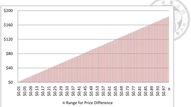
Figure 4.1 Relationship of price difference of two suppliers and holding cost………44

Figure 4.2 The optimal solution under different expected disruption level………….47

Figure 4.3 The analysis of verification by trial and error method………49

Figure 4.4 Sensitivity analysis of price difference of two suppliers………52

Figure 4.5 Sensitivity analysis of holding cost………55

Figure 4.6 Sensitivity analysis of shortage cost………...……57

Figure 4.7 Scenario analyses of two situations………63

VII

LIST OF TABLES

Table 2.1 Category of risk and drivers of risk………..10

Table 2.2 Examples for proactive and reactive measures………12

Table 2.3 Tailored strategies for mitigation approach………..15

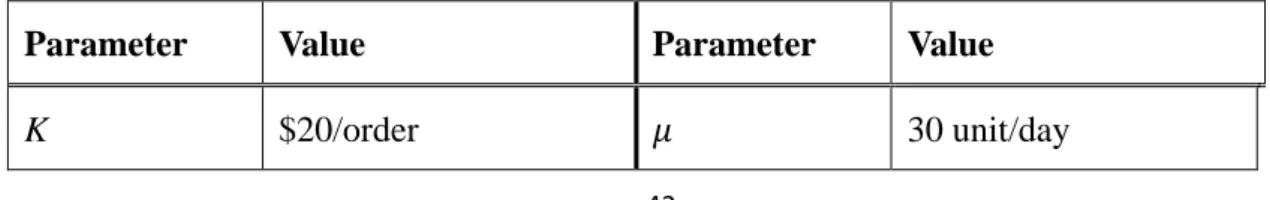
Table 4.1 The parameter settings for retailer………42

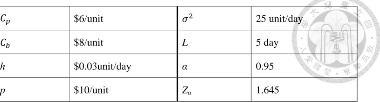
Table 4.2 Other parameter settings for retailer……….43

Table 4.3 The expected disruption level for each risk preference level………...46

Table 4.4 The optimal solution under different expected disruption level…………...46

Table 4.5 The analysis of verification by trial and error method……….49

Table 4.6 Sensitivity analysis of price difference of two suppliers………..51

Table 4.7 Sensitivity analysis of holding cost………..54

Table 4.8 Sensitivity analysis of shortage cost……….57

Table 4.9 Scenario analysis under 100% disruption level………60

Table 4.10 Scenario analysis under 3.5% disruption level………...62

1

Chapter 1 Introduction

1.1 General Background Information

Over the past decades, as technologies and conveyances have been improved, companies are striving to meliorate their financial performance by implementing various supply chain initiatives such as outsourcing and Just-in-Time inventory system.

These initiatives are intended to create extra profit through reducing cost, reducing assets, and increasing revenue. However, while companies implement more supply chain initiatives, the whole supply chain system becomes more complex and uncertain.

According to an industry study conducted by AMR Research in 2006, over 42% of the companies manage more than 5 different supply chains. (AMR, 2006) The increasing number of supply chains which companies have to manage creates difficulty for companies to manipulate perfectly and also makes the impact of any event become hard or even impossible to predict. These kinds of long and complex supply chains are usually slow to respond to changes, and hence, they are more vulnerable to business disruptions. According to a study conducted by Computer Sciences Corporation in 2004, 60% of the firms reported that their supply chains are vulnerable to disruptions.

Therefore, nowadays companies are taking supply chain disruption risk very seriously and trying very hard to avoid it.

2

Many recent events have shown how disruption impacted the supply chain and global industry. For instance, the huge earthquake in Japan, 2011, was a catastrophe which also followed by a nuclear crisis and caused a significant shortage of electricity on electronics industry. Global suppliers of NAND and DRAM were greatly affected by factories shutdown. Toshiba Corp., a consumer electronics device manufacturer, accounting for 35% of flash memory in the world was also suffered in this earthquake.

Figure 1.1 shows that in the second quarter of 2011, Toshiba’s revenue and market share of NAND flash memory dropped dramatically and the company lost more than 6% of market share during that period.

Figure 1.1 Global NAND flash memory revenue market share by quarter.

(Source: Yu-Hsiang Hung, 2013)

Although disruption can be very devastating for companies, if companies can prepare

3

for it in advance, the result of disruption may become not so overwhelming. For

example, back in 2000, Telefon AB L.M. Ericsson, a mobile-phone manufacturer, lost nearly 400 million Euros after their supplier’s semiconductor plant caught on fire. This

supplier was the only provider of Ericsson’s microchips, so when this plant shut down after the fire, Ericsson had no other source of microchips, which disrupted production of mobile-phone. On the other hand, a Scandinavian mobile-phone manufacturer Nokia Corp. was also a major customer of that plant, but Nokia began switching its chip orders to other Japanese and American suppliers almost immediately after fire started.

Therefore, thanks to its multiple-supplier strategy and responsiveness, Nokia’s production suffered little than Ericsson during this crisis. The different outcomes between these two companies show the importance of proactively managing supply chain disruption risk.

Along with the complexity of supply chain evolvement, companies become rigid and hard to response to changes immediately, and hence, become more vulnerable to any possible disruption in the rapidly competitive environment. To protect companies from these risky threats, many researches have been done on studying supply chain risk drivers, sources, and mitigation strategies (Chopra & Sodhi, 2004; Kleindorfer & Saad, 2005; Tang, 2006). These studies focus on specifying risk, distinguishing its sources, and giving some mitigation strategies to reduce the possible impact of disruptions.

4

Based on these former researches, our research is focusing on finding the balance between those mitigation strategies, hoping to pave a way for dealing with supply chain disruption problems by mathematical models, which can give a lead to decision makers about how to place the best decision about proactive mitigation methods when they manage supply chain. Amanda J. Schmitt (2011) points out that mitigation strategies can be combined together to deal with supply chain disruption problems and give customers’

service level protection. But this research stops at giving a proof of the benefits about combining mitigation measures together, and does not mention about the proportion between these strategies. Therefore, our research is going to add this part on combined mitigation methods. While considering two kinds of mitigation strategies, which are safety stock and backup suppliers, and also trying to combine these two methods together to achieve the optimal expected cost under different disruption scenarios. In our mathematical models, this study will show the optimal solutions of the proportions of safety stock and backup suppliers among different scenarios, and hope to shed light on how to distribute disruption mitigation strategies effectively.

1.2 Research Purpose

Based on the above background, our research will integrate topic-related literatures, and try to give a clear outline of supply chain disruption risk and build mathematical models to demonstrate how to adopt disruption mitigation strategies together so as to

5

proactively act on the possible supply chain disruption risk under the lowest cost.

The objectives of this research are:

1. To help decision makers understand how to adopt disruption mitigation strategies effectively and efficiently.

2. To show that the combination of two mitigation strategies, safety stock and backup suppliers, can protect downstream companies effectively when suppliers are all vulnerable to its environment.

3. To demonstrate the benefits of changing proportions of safety stock and backup suppliers under different scenarios.

4. To contribute a literature in building mathematical models for dealing with such supply chain disruption problems.

1.3 Research Scope and Limitation

Although there are lots of mitigation approaches that companies can adopt to their supply chain planning such as production postponement and supply contracts, our research will choose only two mitigation strategies, which are safety stock and backup suppliers, because this study just wants to show that the benefits of combing mitigation strategies together will bigger than only using one mitigation approach alone. Thus, depending on our result of proving the advantage of combination, companies can use as

6

many approaches as they want as long as these are affordable to them and gain benefits from adopting these mitigation strategies together.

This research investigates companies’ expected working inventory cost resulting from different disruption levels by adopting safety stock and backup suppliers approaches together under two-echelon supply chain with stochastic demand, whose inventory-control policy is continuous-review policy, and the probability of a disruption occurring at more than one supplier of the same company simultaneously is negligible and that after a disruption the system returns to steady-state prior to another disruption’s occurrence.

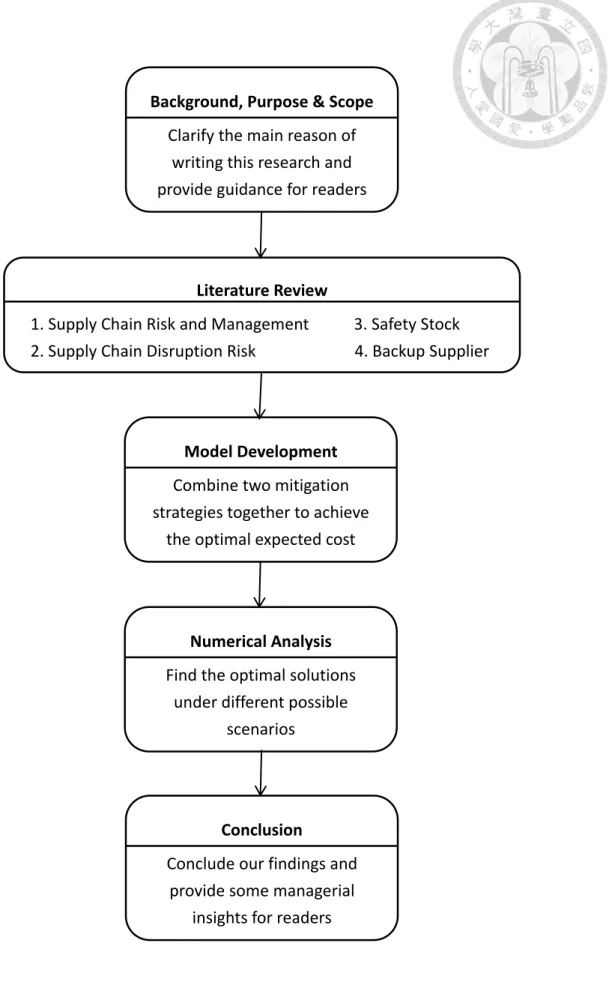
1.4 Research Framework and Process

In this research, first, this study considers the characteristics of safety stock and backup suppliers which are our mitigation strategies. Next, this study shows how these two approaches can be combined together to create the optimal solution of the lowest cost for companies. Furthermore, this study explores under certain scenarios what distribution of these two strategies should be adopted to provide companies’ lowest cost.

This study utilizes numerical analysis to show how the proportions of these two strategies can be affected by different situations. Finally, this study draws conclusions and generates some managerial insights in this research, hoping to give decision makers

7

some clues about supply chain planning.

The structure of this research is organized as following: research background, purpose, scope and framework are presented in Chapter 1. In Chapter 2, this study organizes some related literatures to give clear outlines of supply chain disruption risk and its management, safety stock and backup suppliers. This study introduces the model which combines safety stock and backup supplier mitigation strategies together on two-echelon with stochastic demand to achieve the optimal expected cost in Chapter 3.

Numerical analysis about the proportions of these two mitigation strategies under different scenarios is illustrated in Chapter 4. The conclusion of our research is presented in Chapter 5 followed with some managerial insights that can be useful in practical world. Figure 1.2 shows the flowchart of this research.

8

Figure 1.2 Flowchart of this research.

Literature Review

1. Supply Chain Risk and Management 3. Safety Stock 2. Supply Chain Disruption Risk 4. Backup Supplier

Model Development Combine two mitigation strategies together to achieve

the optimal expected cost Background, Purpose & Scope

Clarify the main reason of writing this research and provide guidance for readers

Numerical Analysis Find the optimal solutions

under different possible scenarios

Conclusion

Conclude our findings and provide some managerial

insights for readers

9

Chapter 2 Literature Review

This research’s purpose is to understand the deployment of supply chain disruption mitigation strategies. In this chapter, this study focuses on four dimensions in literature review: supply chain risk and management, supply chain disruption risk, safety stock, and backup supplier. In each sector, this study gives definitions and related information to depict a clear outline of our research content and hope to lead readers to understand this research better.

2.1 Supply Chain Risk and Management

Risk can be broadly defined as a chance of danger, damage, loss, injury or any other undesired consequences and also can be divided into different types according to how its realization impacts on a business and its environment. (Harland, Brenchley & Walker, 2003) Supply chain risk is one of these risk types. According to Heckmann, Comes and Nickel (2014), although the topic of supply chain risk is being considered as increasingly important, there are only a few authors explicitly defining supply chain risk.

Among these authors, the first to establish a supply chain risk definition were March and Shapire (1987): they define supply chain risk as the “variation in the distribution of possible supply chain outcomes, their likelihood, and their subjective values”. Likewise, Peck (2006) defines supply chain risk as “anything that [disrupts or impedes] the

10

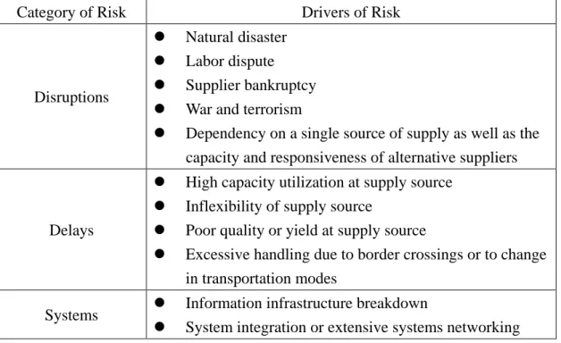
information, material or product flows from original suppliers to the delivery of the final product to the ultimate end-user”. Another research effort by Tang (2006) mentions that supply chain risk should refer to (1) events with small probability but may occur abruptly and (2) these events bring substantial negative consequences to the system. In some researches, authors classify supply chain risk into several categories. According to Tang and Tomlin (2008), they categorize supply chain risk to 6 major types which occur regularly: supply risks, process risks, demand risks, intellectual property risks, behavioral risks, and political/social risks. On the other hand, Chopra and Sodhi (2004) classify supply chain risk into 9 categories, including disruptions, delays, systems, forecast, intellectual property, procurement, receivables, inventory and capacity. This

study shows the details in Table 2.1.

Table 2.1 Category of risk and drivers of risk

Category of Risk Drivers of Risk

Disruptions

 Natural disaster

 Labor dispute

 Supplier bankruptcy

 War and terrorism

 Dependency on a single source of supply as well as the capacity and responsiveness of alternative suppliers

Delays

 High capacity utilization at supply source

 Inflexibility of supply source

 Poor quality or yield at supply source

 Excessive handling due to border crossings or to change in transportation modes

Systems  Information infrastructure breakdown

 System integration or extensive systems networking

11

 E-commerce

Forecast

 Inaccurate forecasts due to long lead times, seasonality, product variety, short life cycles, small customer base

 “Bullwhip effect” or information distortion due to sales promotions, incentives, lack of supply-chain visibility and exaggeration of demand in times of product shortage

Intellectual Property  Vertical integration of supply chain

 Global outsourcing and markets

Procurement

 Exchange rate risk

 Percentage of a key component or raw material procured from a single source

 Industrywide capacity utilization

 Long-term versus short-term contracts Receivables  Number of customers

 Financial strength of customers

Inventory

 Rate of product obsolescence

 Inventory holding cost

 Product value

 Demand and supply uncertainty Capacity  Cost of capacity

 Capacity flexibility

(Source: Chopra and Sodhi, 2004)

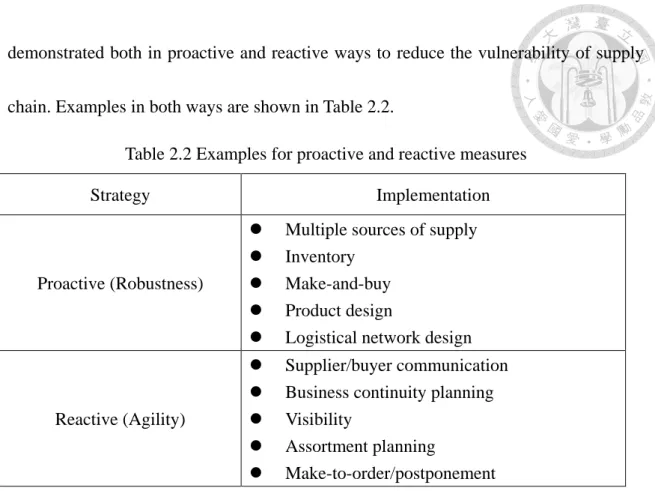
As for supply chain risk management (SCRM), Tang (2006) defines it as “the management of supply chain risk through coordination or collaboration among the supply chain partners so as to ensure profitability and continuity”. In addition, Wieland and Wallenburg (2012) define SCRM as “the implementation of strategies to manage both everyday and exceptional risks along the supply chain based on continuous risk assessment with the objective of reducing vulnerability and ensuring continuity”. And they also mention that SCRM can be seen as being “two-sided coin”, which can be

12

demonstrated both in proactive and reactive ways to reduce the vulnerability of supply

chain. Examples in both ways are shown in Table 2.2.

Table 2.2 Examples for proactive and reactive measures

Strategy Implementation

Proactive (Robustness)

 Multiple sources of supply

 Inventory

 Make-and-buy

 Product design

 Logistical network design

Reactive (Agility)

 Supplier/buyer communication

 Business continuity planning

 Visibility

 Assortment planning

 Make-to-order/postponement (Source: Wieland and Wallenburg, 2012)

Furthermore, Chopra and Sodhi (2004) also introduce some general mitigation approaches as following: increasing capacity, acquiring redundant suppliers, increasing responsiveness, increasing inventory, increasing flexibility, pooling or aggregating demand, and increasing capability. These approaches can be selected by companies after they clearly understand their supply chain risk.

In summary, while the definitions in each research of supply chain risk and SCRM are different and few, it is undoubted that these two issues are becoming more and more popular and there are lots of existing researches related to. By clearly understanding the likely risk in companies’ supply chain, managers can implement the appropriate

13

strategies to eliminate the possible severe outcome in advance or reduce the level of vulnerability afterward.

2.2 Supply Chain Disruption Risk

Disruption is one of supply chain risk types, according to Chopra and Sodhi (2004).

Disruptions can be frequent or infrequent; short- or long-term; and cause problems for the affected organization(s), ranging from minor to serious. Instances of disruption are shown above in Table 2.1. Hou, Zeng and Zhao (2010) define supply chain disruption as the sudden of supply; that is, when unexpected events occur, the main source becomes totally unavailable. And they also describe supply disruption is infrequent risk but has large impact on the whole supply chain, because it could cut off the cash flow and stop the operation of the entire supply chain. In addition, Kleindorfer and Saad (2005) mention that disruption risk can be separated into two categories, which are operational risks (equipment malfunctions, unforeseen discontinuities in supply, human-centered issues from strikes to fraud), and risks arising from natural hazard, terrorism, and political instability. Generally, disruptions often imply the halt of material flow;

therefore, although the occurrence of disruption is rare and unpredictable, it is often quite damaging and destructive.

In this point of view, researches about implementing strategies for mitigating disruption

14

risks become more and more. According to Tang (2005), the property that should be included in mitigation strategies is “Resiliency”, meaning the capability to enable a firm to sustain its operation during a major disruption and recover quickly after a major disruption. Besides, Kleindorfer and Saad (2005) give us a clear outline about how to manage disruption risk. They bring out the three tasks as the foundation of disruption risk management, which are: Specifying sources of risk and vulnerabilities, Assessment and Mitigation (SAM). SAM can be briefly explained by steps like understanding the nature of risks, quantifying them, and then, from the result of risk assessment, integrating appropriate management policies to achieve mitigation. Practical strategies to mitigate disruption risks are introduced in Chopra and Sodhi (2004). They consider the best mitigation strategies against disruption risks are (1) adding inventory and (2) having redundant suppliers. These two strategies are proactive approaches to prevent companies from serious damage resulted from supply chain disruptions. There are two reasons to support the strategy of building inventory according to Chopra and Sodhi (2004). First, building inventory does make sense if the disruption can be predicted with reasonable confidence. For example, if companies have learned the impending labor strike beforehand, they can selectively build up inventories so when supply is disrupted as predicted, damage can be minimized by the extra inventory. Second, stockpiling inventory as a hedge against disruption also makes sense for commodity products with

15

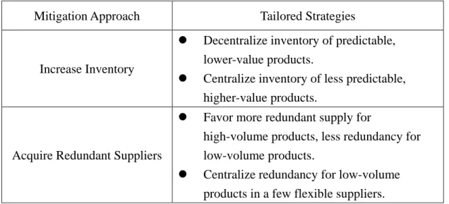
low holding costs and no danger of obsolescence. The large petroleum reserve kept by the United States is a perfect example of this strategy. As for products with high holding costs and/or a high rate of obsolescence, according to Chopra and Sodhi (2004), using redundant suppliers is a better strategy. Motorola Inc., for instance, buys many of its handset components from multiple vendors. In addition, companies can lower the cost of redundancy by using multiple suppliers for high-volume products and single sourcing for low-volume products. This approach helps the company lower the risk of disruption while preserving economies of scale at its suppliers. Chopra and Sodhi (2004) also suggest that companies can tailor their response to disruption risk by considering the cost of reserve and product volumes. Table 2.3 shows the tailoring reserves for

disruption risk mitigation.

Table 2.3 Tailored strategies for mitigation approach

Mitigation Approach Tailored Strategies

Increase Inventory

 Decentralize inventory of predictable, lower-value products.

 Centralize inventory of less predictable, higher-value products.

Acquire Redundant Suppliers

 Favor more redundant supply for

high-volume products, less redundancy for low-volume products.

 Centralize redundancy for low-volume products in a few flexible suppliers.

(Source: Chopra and Sodhi, 2004)

As reported in Kunreuther (1976), many managers tend to ignore possible events that

16

are very unlikely. Thus, companies usually tend to underestimate disruption risk in the absence of accurate supply chain risk recognition. However, through our introduction about disruption risk, this study can believe that the key point for companies to thrive is to find effective strategies to mitigate the risks of supply chain disruption. Since inventory and redundant suppliers are suggested appropriate approaches to cope with disruption risks, this study is continuing to introduce the literatures about these two topics in next two sections.

2.3 Safety stock

The concept of safety stock is often mentioned in inventory management. The definition in Operations Management (2007) of safety stock is that it is stock which is held in excess of expected demand due to variable demand rate and/or lead time.

Another definition of safety stock on BusinessDictionary.com is the inventory held as buffer against mismatch between forecasted and actual consumption or demand, between expected and actual delivery time, and unforeseen emergencies. And it also mentions that safety stock can be called as reserve inventory. According to Stadtler and Kilger (2007), safety stock has to protect against uncertainty which may arise from internal processes like production lead time, from unknown customer demand and from uncertain supplier lead times. They mention that the main drivers for the safety stock

17

level are production and transport disruptions, forecasting errors, and lead time variations. And the benefit of safety stock is that it allows quick customer service and avoids lost sales, emergency shipments, and the loss of good will. Furthermore, safety stock for raw materials enables smoother flow of goods in the production process and avoids disruptions due to stock-outs at the raw material level. Besides the uncertainty mentioned above the main driver of safety stock is the length of the lead time (production or procurement), which is necessary to replenish the stock.

Lots of researches have been done to calculate the optimal safety stock level while considering lead time and demand deviation. One of the most widely accepted methods of calculating safety stock uses the statistical model of standard deviations of a normal distribution of numbers to determine probability. This statistical tool has proven to be very effective in determining optimal safety stock levels in a variety of environments.

Two policies are often introduced in operations management textbooks, which are continuous-review policy and periodic-review policy. In Operations Management (2013), the mathematical models for these two policies are as following:

 Safety Stock in Continuous-Review Policy = Zσ_d√L (Z means service factor

which used as a multiplier with the standard deviation to calculate a specific quantity to meet the specified service level.; σ_d means the standard deviation of demand; L means the fixed lead time).

18

 Safety Stock in Periodic-Review Policy = Zσ_d√P + L (P means predetermined

time which is also the reorder period; P + L represents the protection interval, which is the period over which safety stock must protect the user from running out when there are customer demands).

Graves and Willems (2000) also provide a method to optimize safety stock size. They use periodic-review policy to decide how to place safety stocks across the supply chain to provide 100% service for the assumed bounded demand with the least inventory holding cost. In their single-stage model, they represent safety stock as the expected inventory, which depends on the net replenishment time and the demand bound. They also show multi-stage model and algorithm for spanning tree, and then, conclude this research at giving an application in a real world company. In addition, Qi, Shen and Snyder (2009) use continuous-review policy to decide the optimal safety stock level when under supplier disruptions. They find that (1) when the supplier is always available and the downstream retailer is sometimes disrupted, there is no need to hold safety stock at the retailer. (2) If the retailer is never disrupted but the supplier is sometimes unavailable, the retailer should hold safety stock, and the safety stock level should increase as the availability of the supplier decreases. This point of view supports the concept of using safety stock to avoid the disruptions from upstream suppliers and also gives us a reason to adopt safety stock as a mitigation strategy.

19

In conclusion, there is a large variety of methodological approaches regarding the inventory management processes with disruption risks. Safety stock is one of these approaches. It provides the benefit of protection whether under normal demand fluctuation or emergency disruption situation. Therefore, in our research, we are hoping by adopting safety stock to our model, this study can create the most useful model for decision makers to use when making their supply chain plans.

2.4 Backup supplier

The concept of backup supplier is derived from multiple sourcing strategies. Several researches have proven that multiple sourcing strategies can create benefits when disruption happens, for instance, Burke, Carrillo and Vakharia (2006) and Pochard (2003). According to Gurnani, Mehrotra and Ray (2011), they describe backup supplier like this: Rather than routinely source from multiple suppliers, a firm might instead single source under normal circumstances but rely on an emergency backup supplier in the event of a disruption to its primary supplier. If the emergency backup can respond rapidly when called upon, then an adequate flow of material can be maintained. They also mention that an effective backup sourcing requires proactive planning, and, if necessary, the firm should work to outline better plans to provide backups for certain critical facilities to prevent backups from disruption risk.

20

Lots of researches about backup supplier investigate the usage of contract. Hou, Zeng and Zhao (2010) use buy-back contract to decide the optimal order quantity to backup supplier and the value of using backup supplier. Saghafian and Van Oyen (2011) use option contract to determine the advance capacity investment/reservation level with a flexible backup supplier and the inventory ordering policy of the underlying products from both primary and backup suppliers. And in this research, they also give us a clue about how important it is to have flexible backup suppliers to use. They investigate the value of implementing flexibility in the backup system showing that contracting with a single flexible backup supplier is better rather than contracting with two inflexible ones.

Their study show an average cost reduction of 36%, so flexibility can indeed be highly beneficial; furthermore, it becomes more beneficial as the backup premium increases.

Kouvelis and Li (2008) also consider the same point of view. They show that companies should consider the emergency order like this: the later the delivery of the original order, the higher the possibility of using the flexible backup supply. The flexible backup supply is used only when the delivery of the original order is “late” enough. Therefore, from previous researches, this study finds out that not only the contract is important, but also the flexibility, which can be response time and emergency capacity.

For response time, Gurnani, Mehrotra and Ray (2011) show that the backup strategy profit exhibits increasing returns to response time reductions; that is, the incremental

21

benefit to reducing response time is higher the faster the response time. Furthermore, the nature of the disruption (short-frequent or long-rare) plays a crucial role. The profit falls off rapidly in the case of short-frequent disruption; if the emergency supplier cannot respond very quickly then the backup strategy is not effective at mitigating short-frequent disruptions. The profit falls off much more slowly in the case of long-rare disruptions; therefore, there may be a tradeoff between cost, response time and capacity.

In the case of long-rare disruptions it may make sense to sacrifice some response time to gain on the other dimensions. Besides, Schmitt (2011) also use response time to be a parameter of backup supplier and use it as a variable in model to decide the expected service level.

As for emergency capacity, Gurnani, Mehrotra and Ray (2011) also show that the profit of a company increases gradually as its emergency capacity of backup supplier increases. The amount of available capacity from backup supplier is a crucial factor to company’s profit. Hence, ensuring additional capacity at an external backup source is very important; however, this might require the firm to pay an ongoing fee to reserve a desired level emergency capacity or to contract with multiple suppliers to provide enough backup capacity. In addition, the nature of the disruption also plays a significant role in here. For short-frequent disruptions, the profit is somewhat insensitive to capacity when the response time is long. On the other hand, in the case of rare-long

22

disruptions, the profit increases significantly in capacity even at these longer response times. Therefore, there is a tradeoff between these two flexible factors. If the firm needs short response time, it may face lack of available capacity and vice versa. Thus, simply speaking, when decision makers have to select backup supplier, they can depend on the nature of their possible disruption to deicide the properest backup supplier. For example, response time is a crucial concern for short-frequent disruptions whereas emergency capacity is important for long-rare disruptions.

From these researches, this study notices that response time and emergency capacity play crucial roles in backup supplier strategy; however, in our research, this study will assume our backup supplier is completely flexible, which means it can response quickly to our requirements and always has abundant capacity for us to use, and will not discuss specific details about response time and emergency capacity further in order to simplify the model, but this study suggests that the later research can base on our model and add these two factors to make this model more sophisticated and realistic.

To summarize, supplier diversification and backup sourcing offer alternatives to stockpiling inventory as a means of mitigating disruption risks. By adopting backup supplier strategy, decision makers do not have to stock extra inventory and carry the holding cost. Therefore, this study will use both backup supplier and safety stock in our model and to see which should be adopted more when under different situations.

23

Chapter 3 Combination of Mitigation Methods

In order to deal with unpredictable supply chain disruption problems, lots of researches have proposed some solutions such as adding inventory and having backup suppliers (Chopra and Sodhi, 2004). In addition, many other literatures discuss this topic with various settings. Our research is based on stochastic continuous-review model (Hillier and Lieberman, 2001), focusing on the benefit providing from proactively applying safety stock and backup supplier mitigation strategies before disruptions happen and investigating the adopting proportion of these two mitigation strategies under different scenarios. In first section, this study will define the problem of this thesis and then introducing our research method and purposes. In second section, this study will introduce some assumptions that help our model more easily to be understood. The last segment will show some notations which will be used in mathematical model and then presenting mathematical model for downstream companies who want to prepare for possible supply chain disruption in advance.

3.1 Problem Definition, Research Method and Purpose

3.1.1 Problem Definition

Our model considers with a disruption risk existing in a two-echelon supply chain

24

retailer (which means manufacturer-retailer). In this two-echelon supply chain, the manufacturer, which is also a primary supplier, is vulnerable to its environment and thus, the order quantities of retailer may be affected by any possible disruption risk of this primary supplier. If a possible disruptive event really occurs, there may only a proportion of order quantities can be delivered on time or none of order quantities can be delivered at all. Hence, in our research, this study wants to find out when a retailer is under this circumstance, what the best policy for a retailer will be to organize its mitigation strategies so as to prepare for disruption risk at lowest cost in advance.

3.1.2 Research Method

Our research uses probability expected value method to form the model. In probability theory, the expected value of a random variable is intuitively the long-run average value of repetitions of the experiment it represents. The expected value can be shown as discrete random variable type and continuous random variable type in mathematical expressions. These two types of expected value computation methods are

shown below:

 When 𝑥_𝑖 is a discrete random variable with probability 𝑝_𝑖, computation of the

expected value is

𝐸 = ∑ 𝑥_𝑖∗ 𝑝_𝑖

𝐼

25

x means the resulting value of an event and p means the probability of resulting in

x, which usually ranges from 0 to 1 and can be shown as P ~(0,1).

 When 𝑥_𝑖 is a continuous random variable and its probability distribution admits a

probability density function 𝑓(𝑥), computation of the expected value is 𝐸 = ∫ 𝑥 𝑓(𝑥) 𝑑𝑥

In our research, this study applies discrete random variable type of expected value computation method to find out what the best solution of proportions of safety stock and backup supplier will be so as to achieve the goal of a retailer, which is to have the lowest expected working inventory cost.

3.1.3 Research Purpose

Our purpose of doing this research is to provide an idea of combining different supply chain disruption mitigation strategies together and show that by using this combination strategy, companies can obtain their optimal results. Therefore, this study uses mathematical modeling method to find out the optimal proportions of safety stock and backup supplier when a retailer is under uncertain time of disruption and uncertain available share of order quantities and, meanwhile, also achieves a goal of the lowest working inventory cost.

26

3.2 Basic Assumptions

In our model, this study considers a retailer who has two upstream manufacturers, one of these is the primary supplier and the other one is the backup supplier. Two suppliers and one retailer form a two-echelon supply chain system. In addition, our timeline is one year; thus, this study computes yearly working inventory cost.

In this kind of two-echelon supply chain system, this study wants to understand when uncertain time of disruption and uncertain available share of order quantities exist, what is the optimal proportions of safety stock and backup supplier that a retailer will choose.

Is more proportion of safety stock better or more proportion of order quantity from backup supplier is better.

In order to simplify the model, this study applies some assumptions as below:

(1) This retailer opens 365 days a year, which also means this retailer works every day and receives demands every day.

(2) There is only one product in this model.

(3) The inventory level is under continuous review policy, also known as (Q, R) policy, so its current value always is known.

(4) The retailer uses traditional EOQ model to decide its (Q, R) policy.

(5) Only the primary supplier has lead time, and the lead time is fixed.

(6) The backup supplier does not have lead time, and its capacity can afford retailer’s

27

regular order quantity, which means retailer can receive its order quantities as long as the order quantities do not exceed its regular order quantity.

(7) The demand for withdrawing units from inventory to sell them is uncertain.

However, the probability distribution of demand is known as normal distribution and can be shown as 𝑁~(𝜇, 𝜎²).

(8) If a stockout occurs before the order is received, the excess demand is backlogged, so that the backorders are filled once the order arrives. When a stockout occurs, a fixed shortage cost is incurred for each unit backordered.

(9) A fixed setup cost is incurred each time an order is placed.

(10) A certain holding cost is incurred for each unit in inventory per day.

(11) Each unit of product has fixed procurement cost, and the retailer only has to pay the procurement cost of received quantities.

(12) The procurement cost of backup supplier is always more expensive than the procurement cost of primary supplier.

(13) The probability distribution of occurring disruption in primary supplier is a uniform distribution, and will only occur once in a year and will not occur continuously to next inventory cycle.

(14) The inventory level starts from regular order quantity plus original safety stock in the beginning of a year.

28

3.3 Model Development

3.3.1 Notations

This study introduces some notations that will be used in our model as below:

Notation Meaning

K Fixed setup cost per order for both suppliers

𝐶_𝑝 Procurement cost per unit, including transportation cost, from primary supplier

𝐶_𝑏 Procurement cost per unit, including transportation cost, from backup supplier, and 𝐶_𝑝<𝐶_𝑏

h Holding cost per unit per day held in inventory p Shortage cost per unit of unsatisfied demand D Total yearly demand

d Random demand per day, assumed to be Normal with mean μ, and variance 𝜎², which is shown as 𝑁~(𝜇, 𝜎²)

L Lead time of primary supplier

u The sum of demand during lead time, as a random variable with mean μL, variance 𝜎²L and probability density function 𝛺_𝐿(𝑢)

Q Regular order quantity for primary supplier, Q =√^2𝜇𝐾

ℎ √^𝑝+ℎ

𝑝

θ Proportion of unavailable order quantities that is going to order from backup supplier, ranging from 0~1. As a decision variable.

1-θ Proportion of unavailable order quantities that is going to use additional safety stock, ranging from 0~1

𝜔_𝑖 Random disruption level of primary supplier, ranging from 0~1.

Assumed to be Normal with 3 different mean 𝜋_𝑖 (i= 1,2,3) standing

29

for 3 risk preference levels, which are risk seeking, risk neutral and risk avoidance respectively, and 𝜋₁>𝜋₂>𝜋₃, variance 𝑠²

α Desired service level

Zα Normal distribution service factor based on desired service level N Number of cycles during a year, N= ^𝐷

𝑄

j The cycle that a disruption occurs

𝑅_𝑟 Reorder point at regular situation, 𝑅_𝑟=μL+ Zα𝜎√𝐿+(1 − 𝜃)𝜔_𝑖Q 𝑍_𝑟 Standard score based on 𝑅_𝑟,

𝑍_𝑟= ^{𝑅𝑟−𝜇𝐿}

𝜎√𝐿 = 𝜇𝐿+ 𝑍𝛼𝜎√𝐿+(1−𝜃)𝜔_𝑖𝑄−𝜇𝐿

𝜎√𝐿 = 𝑍_𝛼+^{(1−𝜃)𝜔𝑖𝑄}

𝜎√𝐿

𝑅_𝑑 Reorder point after a disruption occurs at primary supplier, 𝑅_𝑑=μL+ Zα𝜎√𝐿

3.3.2 Disruptive two-echelon supply chain system

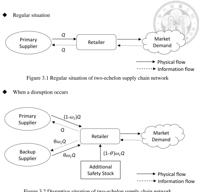
In our model, there are three characters, which are two suppliers, a retailer and market demand from customers. The retailer faces end market demand and has to place orders to its primary supplier regularly. When a disruption occurs to primary supply chain, primary supplier’s delivery will not 100% fulfill the regular order quantity of retailer, which means only (1 − 𝜔_𝑖)𝑄 can be delivered to retailer and the rest of unavailable order quantity 𝜔_𝑖𝑄 will be ordered from backup supplier or use reserved additional safety stock to fulfill the total order quantity Q.

This study shows the system of our model as below:

30

 Regular situation

Figure 3.1 Regular situation of two-echelon supply chain network

 When a disruption occurs

Figure 3.2 Disruptive situation of two-echelon supply chain network

From these two figures above, we can understand that when there is no disruption happens, the flow of entire system is very simple; however, when a disruption occurs, the entire system will become more complex. The retailer has to order the unavailable order quantities from backup supplier to fulfill the rest of regular order quantity. In addition, because our model’s intention is to provide a proactive strategy that can help decision makers find out their best policy of additional safety stock and order quantity from backup supplier in advance, this study has to decide the proportion of ordering

Primary

Supplier Retailer Market

Demand Q

Q

Primary Supplier

Retailer Market

Demand (1-𝜔_𝑖)Q

Q

Backup

Supplier θ𝜔_𝑖Q

θ𝜔_𝑖Q

(1-θ )𝜔_𝑖Q Additional Safety Stock

Physical flow Information flow

Physical flow Information flow

31

from backup supplier θ and the proportion of using reserved additional safety stock (1-θ) in advance before a disruption really happens. Therefore, when a disruption actually occurs, decision makers can follow their predetermined policy of proportions of these two mitigation strategies to place an order quantity to their backup supplier with the lowest cost in working inventory of supply chain.

3.3.3 The expected cost of retailer

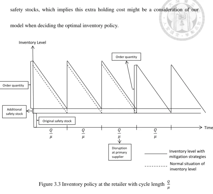
According to the explanation of former section, we can understand that there will be two situations of cost structure in our model. One is ordering from primary supplier of quantity Q as usual; the other one is ordering a partial unavailable quantity from backup supplier and using reserved additional safety stock to fulfill the rest of regular order quantity Q. Before presenting our model, this study wants to show the inventory policy at the retailer first to see how inventory level changes under different situations. In order to simplify the model, this study sets cycle length ^𝑄

𝑑 as expected cycle length ^𝑄

𝜇 and will use the expected cycle length ^𝑄

𝜇 in our mathematical model development.

In Figure 3.3, this study can notice that the inventory level with mitigation strategies is higher than the inventory level in normal situation that is because this study uses additional safety stock as a mitigation strategy. In consequence, our inventory level under this situation will be much higher and with extra holding cost of those additional

32

safety stocks, which implies this extra holding cost might be a consideration of our model when deciding the optimal inventory policy.

Figure 3.3 Inventory policy at the retailer with cycle length ^𝑄

𝜇

Furthermore, from Figure 3.3, this study can also observe that there is a difference in inventory level after a disruption occurs. Before a disruption, the retailer can order from primary supplier at order quantity Q, and at the same time, will also reserve additional safety stock(1 − 𝜃)𝜔_𝑖Q in order to prepare for a sudden disruption at primary supplier.

In our model, because this study uses traditional EOQ model to compute order quantity Q and reorder point R, our original safety stock can be computed as Zα 𝜎√𝐿. Hence, the inventory level before a disruption occurs can be shown as ^𝑄

2+ 𝑍_𝛼𝜎√𝐿 + (1 − 𝜃)𝜔_𝑖Q.

𝑄 𝜇

𝑄 𝜇

𝑄 𝜇

𝑄 𝜇

Original safety stock Additional

safety stock Order quantity

Disruption at primary supplier

Order quantity

Inventory Level

Time

Inventory level with mitigation strategies Normal situation of inventory level

33

On the other hand, because when a disruption happens at primary supplier, it will not affect the inventory level that is already held by retailer; it will only influence the inventory level on next cycle, this study can ensure that even though a disruption occurs at a particular cycle, the inventory level of that cycle will still be ^𝑄

2+ 𝑍_𝛼𝜎√𝐿 + (1 − 𝜃)𝜔_𝑖Q. Only the cycles after a disruption will have different inventory level.

Because for those cycles after a disruption, according to our assumptions, they will not encounter any disruption again during the same year, they do not have to reserve any additional safety stock which means their inventory level can return to normal situation ^𝑄

2+ 𝑍_𝛼𝜎√𝐿.

Based on our previous illustration, this study can introduce our model which will result in the best solution of inventory policy. Our model uses working inventory cost as our objective function. Working inventory cost consists of three types of cost, which are

ordering cost, holding cost and shortage cost, respectively. (Qi, Shen & Snyder, 2009)

 Ordering cost

Ordering cost includes setup cost and procurement cost. In our model, the ordering cost will be different under various situations. The ordering cost per cycle before a disruption happens, which means retailer can place an order Q to primary supplier, will be K +𝐶_𝑝Q. When a disruption occurs at one particular cycle, the ordering cost from primary supplier will be (Q-𝜔_𝑖Q) 𝐶_𝑝+K. In addition, because when under a disruption,

34

the retailer will have to order proportion of unavailable order quantity 𝜔_𝑖Q from backup supplier, the ordering cost from backup supplier will be θ𝜔_𝑖Q𝐶_𝑏+K. The important thing here is that because this study assumes the inventory level starts from

Q+ Zα 𝜎√𝐿, this study has to order additional safety stock at the beginning of year, whose ordering cost will be (1 − 𝜃)𝜔_𝑖Q𝐶_𝑝+K.

 Holding cost

Since this study has introduced the inventory level under different situations previously, this study can now conclude that the holding cost per cycle before a disruption occurs and at a disruptive cycle will be ^𝑄2ℎ

2𝜇 + ^{Zα σ√𝐿𝑄ℎ}

𝜇 +^{(1−𝜃)𝜔𝑖ℎ𝑄2}

𝜇 . On the other hand, the holding cost per cycle after a disruptive cycle will be

𝑄²ℎ

2𝜇 + ^{Zα σ√𝐿𝑄ℎ}

𝜇 .

 Shortage cost

Shortage cost can also be different when under various situations. Before a disruption happens, the retailer will place an order at reorder point 𝑅_𝑟, because the additional safety stock can also be used to compensate demand and be fulfilled again once the order quantity Q arrives. Therefore, the shortage cost per cycle before a disruption occurs will be p∫ (𝑢 − 𝑅_𝑅^∞ _𝑟)

𝑟 𝛺_𝐿(𝑢)𝑑𝑢. When a disruption occurs at a particular cycle, the reorder point will change to 𝑅_𝑑, because retailer has to keep additional safety stock on hand to fulfill proportion of unavailable order quantity that will not be satisfied by

35

backup supplier. Under this circumstance, the reserved additional safety stock cannot be used to compensate lead time demand. Thus, the shortage cost at a disruptive cycle will be p∫ (𝑢 − 𝑅_𝑅^∞ _𝑑)

𝑑 𝛺_𝐿(𝑢)𝑑𝑢. After this disruptive cycle, the retailer can return to its normal situation which means its reorder point will be at 𝑅_𝑑. Therefore, the shortage cost per cycle after a disruption occurs will also be p∫ (𝑢 − 𝑅_𝑅^∞ _𝑑)

𝑑 𝛺_𝐿(𝑢)𝑑𝑢.

In conclusion, the objective function of working inventory cost will be additional safety stock ordering cost at the beginning of year+ working inventory cost before a disruption occurs+ working inventory cost at a disruptive cycle+ working inventory cost after a disruption occurs.

𝐶(𝜃) = (1 − 𝜃)𝜔_𝑖𝑄𝐶_𝑝+ 𝐾 + 𝐾(𝑗 − 1) + 𝐶_𝑝𝑄(𝑗 − 1) +𝑄²ℎ

2𝜇 (𝑗 − 1) + 𝑍𝛼 𝜎√𝐿𝑄ℎ

𝜇 (𝑗 − 1) +(1 − 𝜃)𝜔_𝑖ℎ𝑄²

𝜇 (𝑗 − 1)

+ 𝑝(𝑗 − 1) ∫ (𝑢 − 𝑅_𝑟)

∞

𝑅_𝑟

𝛺_𝐿(𝑢)𝑑𝑢 + (𝑄 − 𝜔_𝑖𝑄)𝐶_𝑝+ 𝐾 + 𝜃𝜔_𝑖𝑄𝐶_𝑏+ 𝐾 +𝑄²ℎ

2𝜇 + Zα σ√𝐿𝑄ℎ

𝜇 +(1 − 𝜃)𝜔_𝑖ℎ𝑄²

𝜇 + 𝑝 ∫ (𝑢 − 𝑅_𝑑)

∞

𝑅_𝑑

𝛺_𝐿(𝑢)𝑑𝑢 + 𝐾(𝑁 − 𝑗) + 𝐶_𝑝𝑄(𝑁 − 𝑗) +𝑄²ℎ

2𝜇 (𝑁 − 𝑗) + 𝑍𝛼 𝜎√𝐿𝑄ℎ

𝜇 (𝑁 − 𝑗)

+ 𝑝(𝑁 − 𝑗) ∫ (𝑢 − 𝑅_𝑑)

∞

𝑅_𝑑

𝛺_𝐿(𝑢)𝑑𝑢 (1)

In our model, 𝛺_𝐿(𝑢) obeys 𝑁~(𝜇𝐿, 𝜎²𝐿), and according to normal distribution characteristics, we can show that

∫ (𝑢 − 𝑅_𝑟)

∞

𝑅_𝑟

𝛺_𝐿(𝑢)𝑑𝑢 = 𝜎√𝐿[𝜓(𝑍_𝑟) − 𝑍_𝑟(1 − 𝛷(𝑍_𝑟))]

36

and

∫ (𝑢 − 𝑅_𝑑)

∞

𝑅_𝑑

𝛺_𝐿(𝑢)𝑑𝑢 = 𝜎√𝐿[𝜓(𝑍_𝛼) − 𝑍_𝛼(1 − 𝛷(𝑍_𝛼))]

𝜓(.) stands for standard normal probability density function, which can be presented as

𝜓(𝑍) = ¹

√2𝜋𝑒^−𝑍22, and 𝛷(.) stands for standard normal cumulative distribution function, which can be presented as 𝛷(𝑍) = ∫_−∞^𝑍 𝜓(𝑡)𝑑𝑡. Therefore, formula (1) can also be written as below

𝐶(𝜃) = (1 − 𝜃)𝜔_𝑖𝑄𝐶_𝑝+ 𝐾 + 𝐾(𝑗 − 1) + 𝐶_𝑝𝑄(𝑗 − 1) +𝑄²ℎ

2𝜇 (𝑗 − 1) + 𝑍𝛼 𝜎√𝐿𝑄ℎ

𝜇 (𝑗 − 1) +(1 − 𝜃)𝜔_𝑖ℎ𝑄²

𝜇 (𝑗 − 1)

+ 𝑝(𝑗 − 1)𝜎√𝐿[𝜓(𝑍_𝑟) − 𝑍_𝑟(1 − 𝛷(𝑍_𝑟))] + (𝑄 − 𝜔_𝑖𝑄)𝐶_𝑝+ 𝐾 + 𝜃𝜔_𝑖𝑄𝐶_𝑏+ 𝐾 +𝑄²ℎ

2𝜇 + Zα σ√𝐿𝑄ℎ

𝜇 +(1 − 𝜃)𝜔_𝑖ℎ𝑄² 𝜇

+ 𝑝𝜎√𝐿[𝜓(𝑍_𝛼) − 𝑍_𝛼(1 − 𝛷(𝑍_𝛼))] + 𝐾(𝑁 − 𝑗) + 𝐶_𝑝𝑄(𝑁 − 𝑗) +𝑄²ℎ

2𝜇 (𝑁 − 𝑗) + 𝑍𝛼 𝜎√𝐿𝑄ℎ

𝜇 (𝑁 − 𝑗)

+ 𝑝(𝑁 − 𝑗)𝜎√𝐿[𝜓(𝑍_𝛼) − 𝑍_𝛼(1 − 𝛷(𝑍_𝛼))] (2) According to our assumption, because the probability distribution of occurring disruption in primary supplier is a uniform distribution, based on uniform distribution characterization, our expected value of working inventory cost will be the working inventory cost of a disruption at first cycle 1 plus the working inventory cost of a disruption at last cycle N, and then dividing by 2. Thus, this can be shown as below:

𝐶(𝜃) = E[𝐶(𝜃, 𝑍)] =𝐶(𝜃) 𝑎𝑡 𝑗 = 1 + 𝐶(𝜃) 𝑎𝑡 𝑗 = 𝑁 2