國立臺灣大學醫學院分子醫學研究所 碩士論文
Graduate Institute of Molecular Medicine College of Medicine
National Taiwan University Master Thesis
有機酸血症的人工智慧判讀輔助系統
The artificial intelligence system to assist interpretation of urine organic acid analysis
馬欽祥 Chin-Shiang Ma
指導教授:李妮鍾 博士
Advisor: Ni-Chung Lee, M.D. Ph.D.
共同指導教授:陳珮珊 博士、賴飛羆 博士 Co-Advisor: Pai-Shan Chen, Ph.D.、Feipei Lai, Ph.D.
中華民國 108 年 7 月
July, 2019
誌謝
在職專班二年的過程彷彿經歷了王國維的人生三境:從『昨夜西風凋碧樹,
獨上高樓,望盡天涯路』到『衣帶漸寬終不悔,為伊消得人憔悴』,最後是『眾裡
尋他千百度,驀然回首,那人卻在,燈火闌珊處』;而準備論文的過程中,從一開
始的看山是山,看水是水,到看山不是山看水不是水,再到看山又是山看水又是 水,其中的滋味,如人飲水,冷暖只有自己知道。
能完成這篇論文,我要特別感謝我的指導教授李妮鍾老師、陳珮珊老師、賴 飛羆老師,也要感謝法醫所華筱玲老師、翁德怡老師,法醫所實驗室的陳儒佑以 及在職專班每一位同學,還有我的家人對我的支持與鼓勵,謝謝大家。
中文摘要
背景
有機酸血症 (Organic acidemia) 是一類會導致急性發病的先天代謝異常疾 病。患者通常在出生後沒多久便會出現代謝性酸中毒、高血氨、高乳酸或低血糖 等症狀,嚴重可能致命。確診後患者必須終身進行飲食控制(低蛋白飲食),並服用 肉鹼以排出有機酸。然而,有機酸血症檢查診斷的判讀極為繁瑣,檢驗操作者及 臨床醫師常需要花費大量的時間在確認物質及判讀。雖然已有自動化化合物標註 的系統,仍需仰賴人力來進行判讀。近年來人工智慧的發展,許多醫療檢驗已可 藉由機器學習來協助臨床檢測。因此,我們希望能利用機器學習建立一套人工智 慧輔助系統來改進有機酸血症的判讀工作,減輕醫事人員的負擔,增進醫療品質,
促進人工智慧對於醫療的應用。
目的
探討以機器學習建立有機酸血症檢測判讀的可行性,促進人工智慧對於醫療 的應用。
資料與方法
我 們 先 收 集 臨 床 報 告 上 診 斷 為 有 機 酸 血 症 患 者 的 氣 相 層 析 質 譜 儀 (Gas chromatography-mass spectrometry; GC-MS)圖譜及化合物相對定量資料,然後進行 疾病確認以及疾病分類的兩階段機器學習,先以卷積神經網路、支持向量機、隨 機森林演算法及深度神經網路進行臨床上匿名的正常樣本及匿名的確診患者之尿 液檢測結果的有機酸資料集進行是否患病的辨認訓練及測試。之後我們再以臨床 確診匿名患者之尿液檢測結果的有機酸資料集進行疾病分類診斷的訓練與測試,
並計算判讀之準確率,以探討機器學習模組對於有機酸血症判讀的可行性。
結果
在是否患病的分辨上,四種機器學習的 F1 值皆可達到 0.8 以上,其中最好的 是深度神經網路 F1=0.84 及 AUC=0.85;在全部 18 種(含正常對照組)有機酸血症疾
病的分類上,卷積神經網路的 F1=0.68,AUC=0.93;在 13 種(含正常對照組)有機 酸血症疾病的分類上(剔除掉四種標誌化合物不在資料集中的有機酸血症疾病和粒 線體疾病),表現最好的是深度神經網路 F1=0.90 及 AUC=0.98,其次為隨機森林分 類法 F1=0.88,AUC=0.97 和支持向量機 F1=0.85,AUC=0.95。
結論
藉由訓練之後的人工智慧模組,證明機器學習可應用在有機酸血症的氣相層 析圖譜及資料判讀,未來將可建立自動化的有機酸血症判讀系統,加速判讀及診 斷,爭取提早治療的時機,並有機會應用到其他常見疾病。
關鍵字:有機酸血症、機器學習、卷積神經網路、支持向量機、隨機森林、深度 神經網路、氣相層析質譜儀、人工智慧
ABSTRACT
Background
Organic acidemias (OAs) is a group of inborn error of metabolism that can have acute metabolic decompensation. Patients with OA usually present with life threatening metabolic acidosis, hyperammonemia, lactic acidemia and hypoglycemia shortly after birth. After diagnosis established, OA patients are suggested to have low protein diet and carnitine supplementation to decrease the organic acid in the body. However, the process for compound identification and interpretation is very tedious. Technicians and physicians need to spend lot of time to working on it. Although automated compound identification software is available, the interpretation still need physician. With the development of artificial intelligence, many laboratory testing tasks can be simplified after applying machine learning technology. Therefore, we plan to develop the artificial intelligence system to assist interpretation of urine organic acid analysis result.
Aim
To set up a module to assist the interpretation of OAs via machine learning, to facilitate the application of artificial intelligence in health.
Materials and methods
We collected chromatograms and compound response ratio data of the gas chromatography-mass spectrometry (GC-MS) from the clinical reports which was diagnosed as OAs. Then the chromatograms and response ratio data from the GC-MS of the anonymous urine sample used to train the Convolution Neural Networks (CNNs)、
Support Vector Machines (SVMs)、Random Forest (RF) and Deep Neural Networks
(DNNs) modules to discriminate disease from normal cases and then perform disease classification. The accuracy and predication rate were calculated to evaluate the feasibility of machine learning in the interpretation of OA.
Result
In disease discrimination, the F1 score of the four machine learning models can reach 0.8 or more, the best of which is the deep neural networks F1=0.84 and AUC=0.85. In terms of disease classification, in all 18 kinds (including the normal control group) OA classification, the performance of convolutional neural network is F1=0.68 and AUC=0.93 ; in 13 kinds (including the normal control group) OA classification (excluding the four OAs whose target compounds doesn’t exist in the dataset and the mitochondrial dysfunction and stress), the deep neural network achieved highest performance F1=0.90 and AUC=0.98,followed by the random forest classification F1=0.88,AUC=0.97 and support vector machine F1=0.85,AUC=0.95.
Conclusion
The models we trained to assist the interpretation of OAs were approved its feasibility. We can build the automatic system to facilitate the diagnosis of OAs, in order to improve the management of these patients, and apply to related fields of diseases in the future.
Keywords: organic acidemia, machine learning, convolution neural network, support vector machine, random forest, deep neural network, gas chromatography-mass spectrometry, artificial intelligence
CONTENTS
口試委員會審定書 ... #
誌謝 ...i
中文摘要 ... ii
ABSTRACT ...iv
CONTENTS ...vi
LIST OF FIGURES ...ix
LIST OF TABLES ... x
Chapter 1 Introduction ... 1
1.1 Organic acidemia ... 1
1.2 Difficulties of the interpretation for organic acidemia ... 2
1.3 Machine learning tools ... 3
1.3.1 Support vector machines (SVMs) ... 3
1.3.2 Random forest (RF) ... 4
1.3.3 Deep neural networks (DNNs) ... 4
1.3.4 Convolution neural networks (CNNs) ... 5
1.4 Application of deep learning in metabolomics ... 6
1.5 Aim ... 7
Chapter 2 Materials and Methods ... 8
2.1 GC-MS data ... 8
2.1.1 Data format ... 10
2.1.2 Data processing ... 11
2.2 Data preparation for machine learning ... 12
2.2.1 Input format for CNNs ... 12
2.2.2 Input format and transformation for SVM, RF and DNNs ... 13
2.3 In-house organic acidemia GC-MS raw data ... 15
2.3.1 GC-MS raw files in NTUH database ... 15
2.3.2 Data augmentation ... 15
2.3.3 Training and testing sets ... 16
2.4 Methods ... 18
2.4.1 Implementation for convolutional neural networks ... 18
2.4.2 Implementation for the support vector machine ... 20
2.4.3 Implementation for the random forest ... 21
2.4.4 Implementation for the deep neural networks ... 21
2.5 Working flow for different machine learning methods ... 22
2.6 Performance evaluation ... 23
Chapter 3 Results ... 24
3.1 Evaluation of the models on non-targeted compounds ... 25
3.1.1 Disease discrimination by CNNs ... 25
3.1.2 Disease categorization by CNNs ... 26
3.2 Evaluation of the models on targeted compounds ... 28
3.2.1 Disease discrimination by SVM/RF/DNNs ... 28
3.2.2 Disease categorization by SVM/RF/DNNs ... 28
3.2.3 5-fold cross-validation result ... 30
Chapter 4 Discussion... 31
4.1 Proposed approach ... 31
4.2 Potential other machine learning methods ... 31
4.3 Limitations ... 32
4.4 Future works ... 34 4.5 Conclusion ... 34 Chapter 5 References ... 36
LIST OF FIGURES
Figure 1 A chromatogram of a urine sample detected by GC-MS system. ... 2
Figure 2 The demonstration of Support Vector Machine ... 3
Figure 3 The demonstration of Random Forest ... 4
Figure 4 The demonstration of Deep Neural Networks ... 5
Figure 5 The demonstration of Convolution Neural Networks ... 6
Figure 6 A concept flowchart of process ... 8
Figure 7 GC-MS data handling ... 9
Figure 8 GC-MS retention time、m/z and abundance ... 10
Figure 9 Chromatogram of a normal urine sample detecting by GC-MS system ... 11
Figure 10 Chromatogram of a 3MCC urine sample detecting by GC-MS system... 15
Figure 11 Concept of CNNs model ... 18
Figure 12 An example of CNNs blocks... 20
Figure 13 Concept of SVM、RF and DNNs model... 21
Figure 14 Workflow for CNNs and SVM/RF/DNNs to disease pattern recognition ... 23
Figure 15 ROC AUC of SVM/RF/DNNs ... 25
Figure 16 Confusion Matrix of CNNs result ... 27
Figure 17 ROC AUC of CNNs result ... 27
Figure 18 Confusion Matrix of DNNs result ... 30
Figure 19 Complicated OA case ... 33
LIST OF TABLES
Table 1 Organic acidemias and related target compounds ... 14
Table 2 Part of the 34 column matrix of the input dataset for SVM/RF/DNNs ... 14
Table 3 Numbers of samples in the dataset for CNNs and SVM/RF/DNNs ... 17
Table 4 Training set for SVM/RF/DNNs ... 17
Table 5 Testing set for SVM/RF/DNNs... 17
Table 6 Classified Performance Summary ... 24
Table 7 Discriminated Performance of CNNs ... 25
Table 8 Classified Performance of CNNs ... 26
Table 9 Discriminated Performance of SVM/RF/DNNs ... 28
Table 10 Numbers of samples in the dataset for SVM/RF/DNNs ... 29
Table 11 Classified Performance of SVM/RF/DNNs ... 29
Table 12 5-fold cross-validation of 13 kinds OAs ... 30
Chapter 1 Introduction
1.1 Organic acidemia
Organic acidemia (OA) is a group of inborn error of metabolism that could lead to metabolic emergency and are caused by defects in that degradation of branched chain amino acids (especial leucine, isoleucine, and valine) (Dionisi-Vici, Deodato et al. 2006, Wendel and Ogier de Baulny 2006). During the degradation of these aminoacids, intermediates harboring CoA residues will be produced. If the following degradation pathway is blocked, the compounds with CoA accumulates and turn to organic acids, and then results in acidification of blood. Of those OAs, Methylmalonic academia (MMA), Propionic academia (PA), Isovaleric acidemia (IVA) are the major diseases (Dionisi-Vici, Deodato et al. 2006, Wendel and Baulny 2006). Patients with OA present may with metabolic acidosis, hyperammonemia, lactic acidosis, and hypoglycemia shortly after birth or under stress (Dionisi-Vici, Deodato et al. 2006, Wendel and Baulny 2006). Emergent hemodialysis is needed for those with hyperammonemia or profound lactic academia (Baumgartner, Horster et al. 2014, Tsai, Hwu et al. 2014). Long-term management includes restriction of protein intake to decrease the synthesis of organic acid, and supplementation of carnitine that helps in urine excretion of organic acids and supply for secondary carnitine deficiency (Stanley, Bennett et al. 2006, Wendel and Ogier de Baulny 2006, Spiekerkoetter, Bastin et al. 2010, Baumgartner, Horster et al.
2014). However, in the circumstance of stress, such as fever, major operation, or infection, patients with organic OA still can present with acute metabolic decompensation such as hyperammonemia and metabolic acidosis that can be life-threatening with various age of onset from newborn to elders. The diagnosis of OA
relies on urine organic acid analysis by Gas chromatography-mass spectrometry (GC-MS) and tandem mass of metabolite (Tanaka, West-Dull et al. 1980, Naccarato, Gionfriddo et al. 2014). Although some automated commercial systems are available (Kimura, Yamamoto et al. 1999), technicians and physicians still need to double check with a tedious, laborious, and time consuming manner.
1.2 Difficulties of the interpretation for organic acidemia
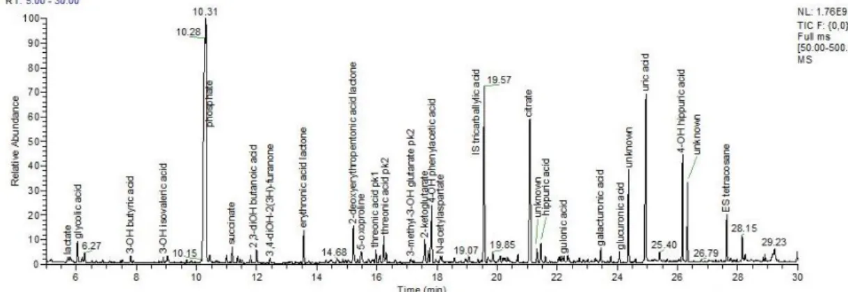
The diagnosis of OAs is usually based on the identification of abnormal metabolic compounds using GC-MS analysis of urine (Naccarato, Gionfriddo et al. 2014). The identification of compounds are based on the retention time (RT) and the mass spectra of the compound (Figure 1). In general, each urine sample usually has 10 to 30 compounds need to identify and the labeling, checking of those compounds is labors. In addition, the diagnosis of specific OA relies on the combination of certain compounds identified that will also need time to group them. Because of the complexity of the above work, it will be very helpful if we can apply the artificial intelligence (AI) in this field. Also, because of the uniqueness of the testing and disease, it is suitable to develop a machine learning model for it.
Figure 1 A chromatogram of a urine sample detected by GC-MS system.
1.3 Machine learning tools
This section covers an overview of the machine learning methods that we applied to GC-MS raw data. We assumed that these methods could be employed to learn OA patterns directly from the raw data. In this study, we propose the use of convolutional neural networks (CNNs), support vector machines (SVMs), random forest (RF) and deep neural networks (DNNs) to learn patterns directly from the dataset.
1.3.1 Support vector machines (SVMs)
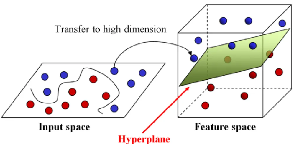
Support vector machines (SVMs) are popular machine learning method and widely and successfully used in classification tasks.(Cortes and Vapnik 1995, Vapnik, Golowich et al. 1996, Chang and Lin 2011) SVMs try to find the high-dimension feature space (hyper-plane) separating the instances of different classes with maximal margin in the optimization process. One limitation of SVMs is the difficulty in determining the best kernel of SVM, whose performance depends on the type of data. Nevertheless, given their success, SVMs were also selected to compare their performance with those of CNNs、RF and DNNs on GC-MS data. (Skarysz, Alkhalifah et al. 2018)
Figure 2 The demonstration of Support Vector Machine (http://i.imgur.com/WuxyO.png)
1.3.2 Random forest (RF)
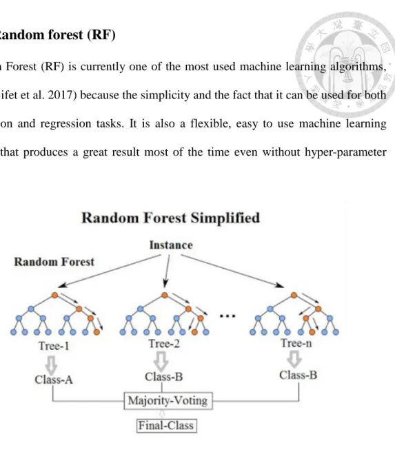
Random Forest (RF) is currently one of the most used machine learning algorithms, (Gomes, Bifet et al. 2017) because the simplicity and the fact that it can be used for both classification and regression tasks. It is also a flexible, easy to use machine learning algorithm that produces a great result most of the time even without hyper-parameter tuning.
Figure 3 The demonstration of Random Forest
(https://medium.com/@williamkoehrsen/random-forest-simple-explanation-377895a60 d2d)
1.3.3 Deep neural networks (DNNs)
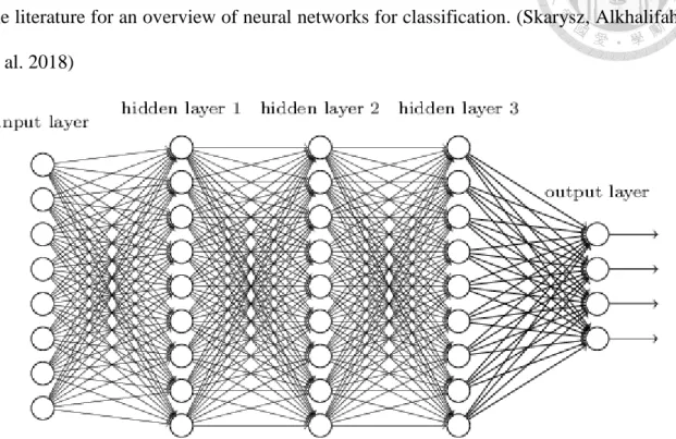
Traditional neural networks (NNs) are widely used to learn a mapping from input to output both for classification and regression tasks. A deep neural network consists of an input layer of neurons, several hidden layer of neurons, and a final layer of output neurons. In this respect, a DNNs is a much simpler structure than a CNNs, but often effective on simple problems. DNNs are known for their ability to learn patterns, and
for this reason were chosen here as a method for comparison with CNNs. Given the popularity of DNNs in machine learning, we omit further general notions and refer to the literature for an overview of neural networks for classification. (Skarysz, Alkhalifah et al. 2018)
Figure 4 The demonstration of Deep Neural Networks (http://neuralnetworksanddeeplearning.com/chap6.html)
1.3.4 Convolution neural networks (CNNs)
Deep learning techniques, especially convolutional neural networks (CNNs) have demonstrated excellent performance in image recognition and classification tasks.
CNNs can autonomously learn useful features directly from low-level data, e.g. pixels, and construct high-level features without human intervention. CNNs can also exploit geometrical properties of the data and are less affected by noise with respect to other techniques. Additionally, an increase of GC-MS as a diagnostic technology will see also an increase of available datasets: a large amount of data is known to benefit the training of deep neural networks. The use of GPU computing and dedicated hardware, which has seen a rapid development in recent years, can help process the large amount of data collected through GC-MS. (Skarysz, Alkhalifah et al. 2018)
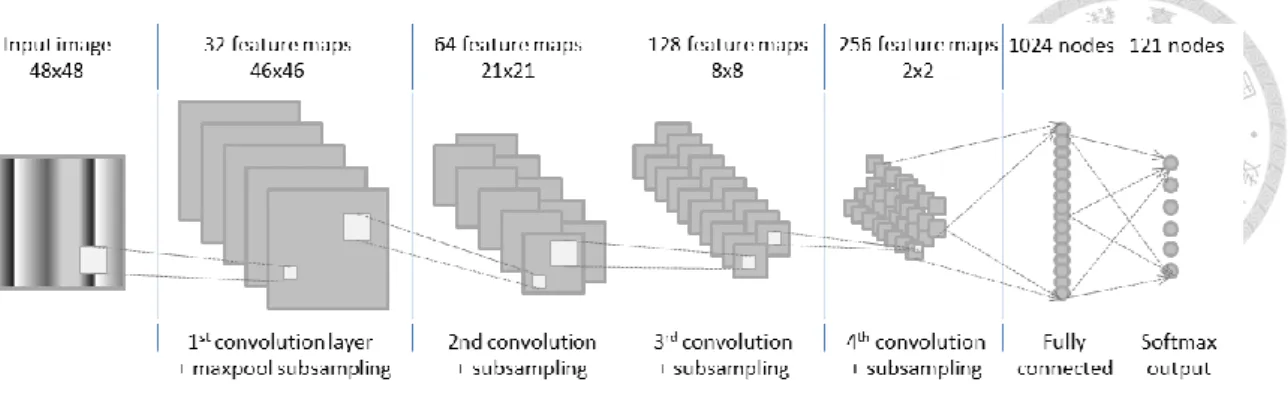
Figure 5 The demonstration of Convolution Neural Networks
(https://blogs.sap.com/2015/01/14/image-classification-with-convolutional-neural-netw orks-my-attempt-at-the-ndsb-kaggle-competition/)
Despite the popularity of the methods described above and their achievements in various fields, their applications in the area of metabolomics are limited and almost exclusively concern preprocessed data. (Skarysz, Alkhalifah et al. 2018)
1.4 Application of deep learning in metabolomics
The diagnosis of OA can be considered as the detecting of abnormal metabolic profiling. The metabolomics has been considered as one of the fields of chemistry and biology in need of machine learning (Date and Kikuchi 2018). The machine learning approach have been successfully applied to nuclear magnetic resonance (NMR) – based metabolomics studies in several disease, such as streptococcus pneumonia infection , devil facial tumor disease, chronic obstructive pulmonary disease, Crohn’s disease, and Celiac disease (Mahadevan, Shah et al. 2008, Bertini, Calabro et al. 2009, Fathi, Majari-Kasmaee et al. 2014, Ravera, Corzilius et al. 2014). In the meanwhile, different deep learning approaches and algorithm had also been used to improve the accuracy of determination, such as knowledge discovery by Regression algorithms, Baysian algorithms, Dimensionality reduction algorithms, accuracy maximization
(KODAMA) and deep neural networks (DNNs), (Cuperlovic-Culf 2018, Date and Kikuchi 2018). Although there had been an attempt to explore feasibility of automated GC-MS biomarkers detection, but the sample size is only 22 normal and 13 abnormal samples (McGarry, Bartlett et al. 2008). Since this is a disease with standard clinical practice need, it will be very useful if we can develop a module to assist the
interpretation of OA.
1.5 Aim
In this study, we set up a model to assist the interpretation of OA via machine learning, to facilitate the application of artificial intelligence in health.
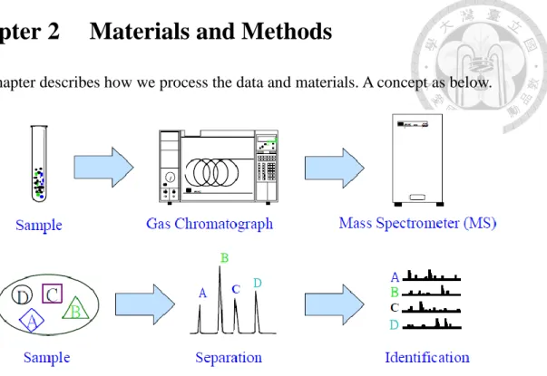
Chapter 2 Materials and Methods
This chapter describes how we process the data and materials. A concept as below.
Figure 6 A concept flowchart of process (Source: ThermoFisher manual)
2.1 GC-MS data
GC-MS is a widely applied technique in many branches of science and technology that is the golden rule for biomarkers discovery. GC-MS will be performed using standard method - 1mL urine (with spikes with different concentration of standards) will be processed by adding each standard 200-250 nmoles and then internal standard (tricarballylic acid 10 mM) 20 μL. Then 5% hydroxylamine HCl (pH7) 100 μL will be added for deriviation in room temperature for 20 minutes to convert keto group to oxime group. After that, 2mL deioninzed water will be added. Solid phase extraction will be performed by Zymark extractor using Waters Sep-Pak 3 (500 mg) AcellTM Plus QMA cartridges. The column will be conditioned by 3mL ethanol and 3mL deionized water followed by urine previously prepared. Then, 6mL 20% ethanol and 1mL hexane
will be used to wash and finalized with 2mL ethanol with 5% formic acid. The flow rate will be 2-3 ml/min. The 20μL tetracosane will be added to the collected eluent and they dried by N2 in 40℃. The dried sample will add 50μL BSTFA + 1% TMCS in 80
℃ for 20 minutes and then diluted 10 times by acetonitrile for injection. 1 μL prepared sample will be injected into GCCS (Thermo Ultra-ISQ) spectrometry through a 1079 injector kept at 280 °C in splitless mode (2 min) and then increment of temperature of 6°C/min up to 200°C and then 12°C/min up to 295°C for 6 minutes. Total time will be 36 minutes. The MS condition will be transfer line 280°C, ion source 280°C, scan by total ion chromatograph, TIC, mx/50-550 and SIM (selected ion monitoring) mode for unknown standards.
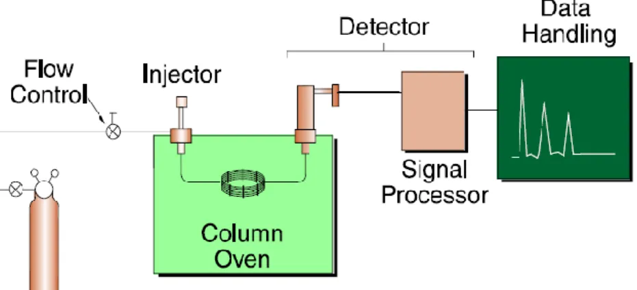
Figure 7 GC-MS data handling (Source: ThermoFisher manual)
The data interpretation will be performed by Xalibur and Tracefinder by interpreting the retention time (RT) and mass spectrum from each compounds.
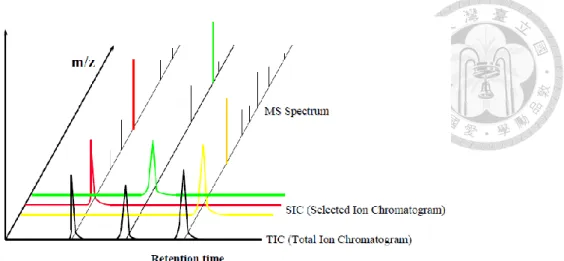
Figure 8 GC-MS retention time、m/z and abundance (Source: ThermoFisher manual)
2.1.1 Data format
GC-MS data can be analysed in either a non-targeted or targeted approach.
Non-targeted analysis is the study of all detected metabolic compounds and their variability to discover potential biomarkers associated with specific organic academia disease. In targeted analysis, a defined panel of metabolic compounds (in this study we will use 34 identified compounds) is sought to detect compounds of interest. ( which are called organic academia biomarkers) (Hiller, Hangebrauk et al. 2009)
In this study, the chromatogram produced by GC-MS is for non-targeted approach.
(Figure 9). The relative abundance on the y-axis, called total ion chromatogram (TIC) is the sum of the intensities compared to internal standard across all m/z measured at the same time, i.e. at a specific retention time point (x-axis). Each peak generally represents one specific metabolic compound, although superposition of peaks occasionally occurs.
Figure 9 Chromatogram of a normal urine sample detecting by GC-MS system As well as the chromatogram, the GC-MS software (here we use ThermoFisher TraceFinder) can provide the response ratio data with 34 identified compounds in each sample. And we will use the data for targeted analysis.
2.1.2 Data processing
Data processing is very critical for machine learning, especially when the data contain abundant information. GC-MS can produce high dimensional, noisy data, for example one single sample can contain over 9 million high-resolution variables.
(Skarysz, Alkhalifah et al. 2018) Usually for clinical interpretation, the chromatogram will be cropped from the GC-MS software and annotated with identified compounds in peaks, which is a highly subjective and laborious task. But in this study we used the chromatogram directly cropped from the GC-MS software without annotation. This process saved a lot of time and manpower. And these chromatogram images were used for CNNs machine learning.
Nevertheless, the chromatogram although noisy and complicated, present unique features that distinguish them. The original idea in this study was that such features can be learned using advanced machine learning techniques like CNNs, directly from raw
GC-MS data and therefore bypassing highly complex preprocessing step. The rest of the paper will cover this idea.
For the SVM、RF and DNNs machine learning, the list of metabolic compounds and their response ratio were the input for a further multivariate statistical analysis, in which the objective was to identify metabolic compounds and their pattern that discriminate between different OAs.
The number of steps and the complexity of the process described above may lead to some challenges. For example, the choice of the best algorithm to baseline identification.
Furthermore, the preprocessing has the potential to introduce errors and variability.
But no matter chromatogram or list compound data are from the same GC-MS raw data, which means they are just the different type or contain different information in the same urine sample.
2.2 Data preparation for machine learning
This section provide the approaches to prepare the suitable format and transformation data for CNNs and SVMs, RF and DNNs. In the beginning we tried to collect the clinical urine samples and used GC-MS to get the data for this study, but it was hard to get enough samples. So we changed our strategy to collect the clinical reports which were diagnosed to OAs in Nation Taiwan University Hospital (NTUH) database. Then we traced back their GC-MS raw files and used the GC-MS raw files to generate the chromatograms and response ratio data. This study was approved by IRB (No. NTUH 201808009RINC).
2.2.1 Input format for CNNs
For CNN image dataset, due to the specific structure of the data, the pattern of each
metabolic compound is contained only in a small portion of the chromatogram, corresponding to a specific range of retention time. Applying current methods and with the supervision of experts, the exact retention time for each target compound and its classification were determined. This process generated a CNN image dataset of labelled OAs of raw data. To link processed with raw data, a dataset structure was created with the following folders: OA, OA_samples, Train, Validation, Test. OA is the name of the folder that contains all clinical organic acidemia urine samples; OA_samples is the name of the folder that classify different OAs in its folders, e.g. 3MCC; train, validation and test are the folder names for machine learning dataset.
Machine learning is a computing resources consuming process. Due to our notebook’s computing power constrain, the image resolution format were limited to 366x966 RGB or 300x900 RGB depending on the CNNs configuration and notebook’s computing resource limitation.
2.2.2 Input format and transformation for SVM, RF and DNNs
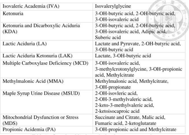
For the SVM, RF and DNN dataset, we collected the response ratio of 34 identified compounds in each urine sample’s GC-MS raw file from different organic acidemias cases. (Table 1.)
Organic Acidemias Target Compounds
3-methylcrotonyl-CoA-Carboxylase deficiency (3MCC)
3-methylcrotonylglycine Aromatic L-amino acid decarboxylase
(AADC)
Vanillylactic acid
Alkaptonuria (AKU) Homogentisate acid
Dicarboxylic Aciduria (DA) Adipic acid, Suberic acid and Sebacic acid, Octanedioic acid, 7-OH octanoic acid, 3-OH-sebacic acid
Ethylmalonic Aciduria (EA) Ethylmalonic acid, Methylsuccinic acid Glutaric Aciduria type 1 (GA1) Glutaric acid and 3-OH-glutarate Glutaric Aciduria type 2 (GA2) 2-OH-gutaric acid, Glutaric acid,
3-OH-butyruc acid, Ethylmalonic acid, Dicarbocylic acids (adipic acid)
Isovaleric Academia (IVA) Isovalerylglycine
Ketonuria 3-OH-butyric acid, 2-OH-butyric acid,
3-OH-isovaleric acid Ketonuria and Dicarboxylic Aciduria
(KDA)
3-OH-butyric acid, 2-OH-butyric acid, 3-OH-isovaleric acid, Adipic acid, Suberic acid
Lactic Aciduria (LA) Lactate and Pyruvate, 2-OH-butyric acid, 3-OH-butyric acid
Lactic Aciduria Ketonuria (LAK) Lactate, 3-OH-butyric acid Multiple Carboxylase Deficiency (MCD) 3-OH-isovaleric acid,
3-methylcrotonylglycine, 3-OH-propionic acid, Methylcitrate
Methylmalonic Acid (MMA) Methylmalonic acid, Methylcitrate, 3-OH-propionate
Maple Syrup Urine Disease (MSUD) 2-OH-isovleric acid,
2-OH-3-methylvaleric acid, 2-keto-3-methylvaleric acid, 2-ketoisocaproic acid Mitochondrial Dysfunction or Stress
(MDS)
Succinate and Citrate, Malic acid, Fumaric acid, 2-ketoglutarate
Propionic Acidemia (PA) 3-OH-propionic acid and Methylcitrate Table 1 Organic acidemias and related target compounds
And then transformed these data into a 34 column matrix as the input for SVM、RF and DNNs.(Table 2.)
Table 2 Part of the 34 column matrix of the input dataset for SVM/RF/DNNs
2.3 In-house organic acidemia GC-MS raw data 2.3.1 GC-MS raw files in NTUH database
The data used in this study was obtained from 690 diagnosed patients (total 727 samples) with different types of OAs and normal cases (no specific finding) in NTUH database. The target compounds in this study were various because different OAs may have different compounds as listed in Table 1. The SVM, RF and DNN dataset contained the response ratio of 34 identified compounds as listed in the first raw of Table 2.
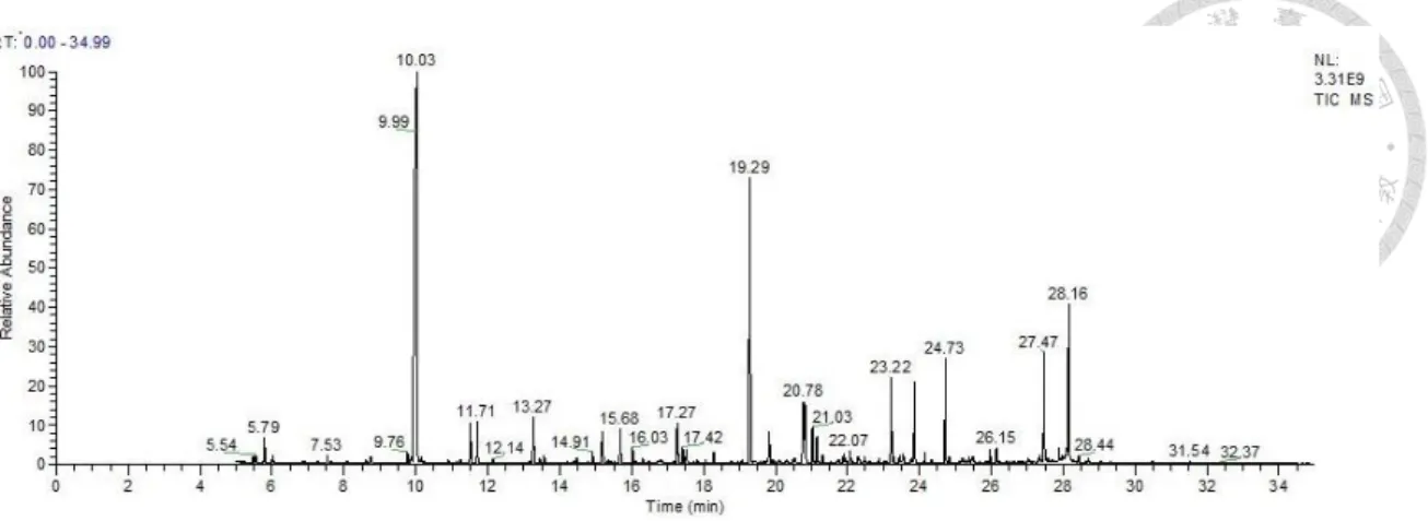
The CNN image dataset contained 721 chromatogram images from 690 diagnosed patients with different types of OAs and normal cases (no specific finding).Below is an example of a chromatogram of a 3MCC urine sample detected by GC-MS system.
Figure 10 Chromatogram of a 3MCC urine sample detecting by GC-MS system
2.3.2 Data augmentation
To increase the robustness of the training and compensate for the limited number of data, data augmentation was applied. (Skarysz, Alkhalifah et al. 2018) We used Keras data generator “ImageDataGenerator” to increase the training images for CNNs by random transformation of the original images in the range: width_shift_range=0.2, height_shift_range=0.2, shear_range=0.2, zoom_range=0.2, Such an augmentation
changes the absolute values of images without changing their proportion, i.e. the pattern.
This augmentation step was repeated to obtain enough additional images for training the CNNs, so the network will never see the same input twice. But the inputs it saw were still heavily intercorrelated, because they come from a small number of original images—we didn’t produce new information, we could only remix existing information.
For the SVM, RF and DNN dataset, due to the limited number of data especially for some disease as AADC, GA1, PA ...etc., we needed to augment the data for training as well. We calculated the means and standard deviations of the original samples and expected it is normal distribution. Then we generate the training dataset randomly by 0.25SD (standard deviation). So the training dataset was generated artificially, not the true data from GC-MS raw files in NTUH database.
2.3.3 Training and testing sets
The CNN image dataset was randomly divided into training、validation and testing set in the proportion around 3:1:1. The training set contained 441 samples, while the validation and testing set contained 140 samples each.
The SVM、RF and DNN dataset used the artificially generated data as training dataset and take the original sample data as testing dataset.
Category CNNs SVM/RF/DNNs
Label Disease Train Validation Test Train Test
0 3MCC 11 4 4 10088 9
1 AADC 4 1 1 10088 3
2 AKU 4 1 1 10088 4
3 DA 15 5 5 10088 18
4 EA 2 1 1 10088 4
5 GA1 5 1 1 10088 4
6 GA2 12 3 3 10088 17
7 IVA 5 1 1 10088 3
8 Ketonuria 9 2 2 10088 14
9 KDA 14 4 4 10088 25
10 LA 11 3 3 10088 20
11 LAK 3 1 1 10088 8
12 MCD 7 2 2 10088 6
13 MMA 16 5 5 10088 21
14 MSUD 5 1 1 10088 5
15 MDS 45 14 14 10088 85
16 PA 6 1 1 10088 6
17 normal 267 90 90 10088 475
Total 441 140 140 181584 727
Table 3 Numbers of samples in the dataset for CNNs and SVM/RF/DNNs
The statistics of SVM/RF/DNN training and testing dataset are listed in the Table 4 and Table 5.
Table 4 Training set for SVM/RF/DNNs
Table 5 Testing set for SVM/RF/DNNs
The inequality of the groups (imbalance dataset) results from the fact that each of the considered OAs has different prevalence.
2.4 Methods
We used different machine learning models to perform the disease discrimination and classification, the confusion matrix and AUC was used to evaluate the performance of different machine learning methods and then used the accuracy, precision, recall and F1_score to compare the performance of different machine learning models.
In this study, we used Python as our programming language. Basically, the standard Keras utilities and Tensorflow backend were used to build up the different machine learning models. We also use the Nvidia CUDA toolkit to perform GPU acceleration.
Figure 11 Concept of CNNs model
2.4.1 Implementation for convolutional neural networks
With GC-MS chromatogram, a geometrical correlation occurs in the retention time dimension. Along this dimension, the response ratio of different m/z increases and decreases thereby creating peaks as the compounds exit the column. So we tested two types of filters: two- dimensional filters, and specific one-dimensional filters along the RT axis only. In the case of two-dimensional filters, sizes were set to (3,3) and (2,2) for
convolution and pooling layers. In the case of one-dimensional filters, sizes were set to (3,1) and (2,1). (Skarysz, Alkhalifah et al. 2018) The convolution neural network architecture was built to stack multiple convolutional layers with ReLU activation before pooling layers. (Figure 12) Several variants of the architecture were tested in preliminary experiments; each was based on the similar layered block consisted of four to seven convolutional layers, pooling layer and dropout layer with rate 0.5. The tested architectures were built of respectively four, five and six such blocks, followed by a fully connected layer with ReLU activation, dropout layer with rate 0.5 and the fully connected layer with softmax activation. The batch size、steps per epoch and the number of epochs were set up as 7、63 and 100 respectively. The results of these preliminary tests gave similar performance among these three architectures. The network with the best performance resulted to be the smallest with two convolutional layers. The best architecture was selected for the experiments in the rest of the paper. We recognized that further, more thorough investigations on the types of architectures and their parameters are interesting future research directions.
Figure 12 An example of CNNs blocks
2.4.2 Implementation for the support vector machine
We used the sckikt-learn module to build the support vector machine. Scikit-learn is a Python module for machine learning built on top of SciPy. In the sklearn.svm module, we used the SVC function with parameter C=1.0, cache_size=200, class_weight=None, coef0=0.0,probability=False,shrinking=True,tol=0.001,decision_function_shape='ovr', degree=3,gamma='auto_deprecated', kernel='rbf', max_iter=-1, random_state=None,
verbose=False.
Figure 13 Concept of SVM、RF and DNNs model
2.4.3 Implementation for the random forest
We used the scikit-learn module to build the random forest model. A random forest is a meta estimator that fits a number of decision tree classifiers on various sub-samples of the dataset and uses averaging to improve the predictive accuracy and control over-fitting. In the scikit-learn package we used the ensemble module to build up the random forest model, we used the RandomForestClassifier function with the parameter n_estimators = 100 and n_jobs=-1 to utilize the two CPU cores at the same time.
2.4.4 Implementation for the deep neural networks
For the DNNs implementation in this study, we used the modules like models, layers
and optimizers in Keras and the function like sequential, dense, activation,dropout,SGD and RMSprop in these modules and used the Tensorflow as the backend. The DNNs used the sigmoid activation function in the hidden layer and softmax activation function for output layer. The size of hidden layer was set up as 2 or 1 and the network was trained with backpropagation as well as learning rate lr=0.001 with RMSprop or lr=0.01 with SGD.
2.5 Working flow for different machine learning methods
All of our data are from the NTUH GC-MS database, we utilized the GC-MS raw files to transfer the raw data to chromatogram and response ratio by TraceFinder. And then used the chromatogram images as the training、validation and testing dataset for CNNs. On the other hand, we utilized the same raw files to transfer the raw data to response ratio (it’s the related abundance compared to internal standard compound) and used these response ratio of 34 identified compounds as the training and testing dataset for SVM、RF and DNNs. Then the training and testing dataset were used to train the different models to get their performance in evaluation metrics. Comparing these evaluation metrics, we can get most promising machine learning model for OA discrimination and categorization.
Figure 14 Workflow for CNNs and SVM/RF/DNNs to disease pattern recognition
2.6 Performance evaluation
Some common evaluation metrics were evaluated (accuracy, precision, recall, and F1 score). The sklearn.metrics.roc_auc_score function were used for depicting the receiver operating characteristic (ROC) curves and calculated the area under the curve (AUC). To evidence the relationships existing between these predictive variables, a confusion matrix was built using the sklearn.metric.confusion_matrix function in scikit-learn module. Total four machine learning evaluation metrics were compared to judge which one achieved the highest performance.
Chapter 3 Results
This section presents the results of discrimination and categorization of the CNNs, SVM, RF and DNNs models using the GC-MS data. All systems were run on Acer Aspire E5-575G notebook running Windows10 64-bit operating system with 2 cores intel i7-6500U [email protected], 16GB RAM and NVIDIA GeForce GTX950M GPU.
The DNNs achieved the highest F1 score 0.90 and the AUC(micro) 0.98 in all machine learning methods we tested. Table 6 summarized the overall performance of different machine learning models and Figure 15 showed the ROC AUC of SVM、RF and DNNs. The detail result would be described in 3.1 and 3.2 section. We used a multiclass classifier called OneVsRestClassifier to calculate the AUC. The AUC(micro) is the global calculation metrics by considering each element of the label indicator matrix as a label and the AUC(macro) is the global calculation metrics for each label, and find their unweighted mean. AUC(macro) does not take label imbalance into account. So we used AUC(micro) to judge the AUC performance between different machine learning models.
Classified Performance Summary
Category Method accuracy precision recall F1 score AUC(macro) AUC(micro)
18 Kinds CNN-1D 0.70 0.56 0.7 0.62 0.66 0.91
18 Kinds CNN-2D 0.72 0.66 0.72 0.68 0.76 0.93
14 Kinds SVM 0.74 0.78 0.74 0.74 0.90 0.91
14 Kinds Random Forest 0.76 0.81 0.77 0.75 0.94 0.92
14 Kinds DNN 0.76 0.86 0.77 0.77 0.95 0.93
13 Kinds SVM 0.83 0.88 0.83 0.85 0.92 0.95
13 Kinds Random Forest 0.87 0.91 0.87 0.88 0.97 0.97
13 Kinds DNN 0.89 0.92 0.89 0.90 0.97 0.98
Table 6 Classified Performance Summary
Figure 15 ROC AUC of SVM/RF/DNNs
3.1 Evaluation of the models on non-targeted compounds 3.1.1 Disease discrimination by CNNs
In the total 721 samples, 174 normal sample chromatogram images and 174 abnormal sample chromatogram images were used to train the CNNs to discriminate the disease from normal cases and these 348 images were augmented in the range of 20% of width and height. Then 137 normal and 50 abnormal chromatogram images were used for validation. The rest 136 normal and 50 abnormal chromatogram images were used for testing the CNNs. The CNNs showed the capability to discriminate the disease.
Category CNNs Discriminated Performance Precision Recall F1-score
Normal 0.93 0.76 0.84
Abnormal 0.57 0.84 0.68
Micro Avg 0.78 0.78 0.78
Macro Avg 0.75 0.80 0.76
Weighted Avg 0.83 0.78 0.80
Table 7 Discriminated Performance of CNNs
3.1.2 Disease categorization by CNNs
We use 441 chromatogram images directly from GC-MS raw data to train the CNNs and 140 chromatogram images for validation and 140 chromatogram images for testing.
From Table 3 we know the data is imbalanced and some OAs samples is very rare, so it do impact the result of CNNs performance. Although the result is unsatisfied, it does show that CNNs could be trained to classify different OA chromatogram patterns. The 1D performance is poor than 2D, so we only listed the 2D result in below table.
Category CNNs Classified Performance Precision Recall F1-score
3MCC 1.00 0.25 0.40
AADC 0.00 0.00 0.00
AKU 0.00 0.00 0.00
DA 0.00 0.00 0.00
EA 0.00 0.00 0.00
GA1 0.00 0.00 0.00
GA2 0.00 0.00 0.00
IVA 0.00 0.00 0.00
Ketonuria 0.00 0.00 0.00
KDA 0.40 0.50 0.44
LA 0.67 0.67 0.67
LAK 0.00 0.00 0.00
MCD 0.00 0.00 0.00
MMA 0.40 0.40 0.40
MDS 0.00 0.00 0.00
MSUD 0.39 0.50 0.44
PA 0.00 0.00 0.00
normal 0.85 0.97 0.91
Micro Avg 0.72 0.72 0.72
Macro Avg 0.21 0.18 0.18
Weighted Avg 0.66 0.72 0.68
Table 8 Classified Performance of CNNs
The confusion matrix of CNNs showed that some OAs were not able to be discriminated may due to the rare training samples and computing power constrain.
With more computing resource we may try more complicated architecture or algorithm to get better performance.
Figure 16 Confusion Matrix of CNNs result
Figure 17 is the ROC AUC of CNNs testing result, the performance is unsatisfied due to the rare imbalanced data.
Figure 17 ROC AUC of CNNs result
3.2 Evaluation of the models on targeted compounds 3.2.1 Disease discrimination by SVM/RF/DNNs
In the total 727 samples, there are 475 normal samples and 252 OA samples. We use 0.25SD to augment the training dataset to 36992 samples, half normal sample and half OA samples. And then used the original 727 samples as testing dataset.
Table 9 shows the discriminated-wise performance of SVM, RF and DNN and the DNN achieved the highest accuracy 0.84 and F1 score 0.84.
Category SVM Performance RF Performance DNNs Performance
Samples Precision Recall F1-score Precision Recall F1-score Precision Recall F1-score
Normal 0.87 0.84 0.86 0.92 0.76 0.83 0.87 0.88 0.88 475
Abnormal 0.72 0.77 0.74 0.66 0.88 0.75 0.77 0.76 0.76 252
Micro Avg 0.82 0.82 0.82 0.80 0.80 0.80 0.84 0.84 0.84 727
Macro Avg 0.80 0.80 0.80 0.79 0.82 0.79 0.82 0.82 0.82 727
Weighted Avg 0.82 0.82 0.82 0.83 0.80 0.80 0.84 0.84 0.84 727
Accuracy 0.82 0.80 0.84 727
Table 9 Discriminated Performance of SVM/RF/DNNs
3.2.2 Disease categorization by SVM/RF/DNNs
Due to the AADC、AKU、DA and MSUD’s target compounds are not listed in the 34 identified compounds and MDS will confuse the training model, so we exclude them from the dataset for SVM、RF and DNNs.
Table 10 shows the numbers of samples in the dataset for SVM/RF/DNNs and we used the same way to generate the training set (data augmentation).
Category SVM/RF/DNNs
Label Disease Train Test
0 3MCC 10088 9
1 EA 10088 4
2 GA1 10088 4
3 GA2 10088 17
4 IVA 10088 3
5 Ketonuria 10088 14
6 KDA 10088 25
7 LA 10088 20
8 LAK 10088 8
9 MCD 10088 6
10 MMA 10088 21
11 PA 10088 6
12 normal 10088 475
Total 131144 612
Table 10 Numbers of samples in the dataset for SVM/RF/DNNs
We have tried different loss functions and optimizers and Table 11 shows the best performance was achieved by DNNs.
Category SVM Performance RF Performance DNNs Performance
Samples Precision Recall F1-score Precision Recall F1-score Precision Recall F1-score
3MCC 1.00 0.33 0.50 1.00 0.67 0.80 1.00 0.56 0.71 9
EA 0.29 1.00 0.44 0.57 1.00 0.73 0.38 0.75 0.50 4
GA1 0.25 0.25 0.25 0.67 1.00 0.80 0.60 0.75 0.67 4
GA2 0.40 0.47 0.43 0.92 0.71 0.80 0.69 0.53 0.60 17
IVA 0.10 0.67 0.17 0.27 1.00 0.43 0.13 0.67 0.22 3
Ketonuria 0.62 0.57 0.59 0.60 0.64 0.62 0.79 0.79 0.79 14
KDA 0.73 0.44 0.55 0.73 0.64 0.68 0.89 0.68 0.77 25
LA 0.62 0.65 0.63 0.34 0.75 0.47 0.67 0.80 0.73 20
LAK 0.33 0.25 0.29 0.64 0.88 0.74 0.80 0.50 0.62 8
MCD 0.40 0.67 0.50 1.00 0.83 0.91 0.30 0.50 0.37 6
MMA 0.46 0.62 0.53 0.83 0.48 0.61 1.00 0.52 0.69 21
PA 1.00 0.83 0.91 1.00 1.00 1.00 1.00 0.83 0.91 6
normal 0.96 0.92 0.94 0.96 0.92 0.94 0.96 0.96 0.96 475 Micro Avg 0.83 0.83 0.83 0.87 0.87 0.87 0.89 0.89 0.89 612 Macro Avg 0.55 0.59 0.52 0.73 0.81 0.73 0.71 0.68 0.66 612 Weighted Avg 0.88 0.83 0.85 0.91 0.87 0.88 0.92 0.89 0.90 612
Accuracy 0.8349 0.8741 0.8921 612
Table 11 Classified Performance of SVM/RF/DNNs
The confusion matrix shows as below.
Figure 18 Confusion Matrix of DNNs result
3.2.3 5-fold cross-validation result
Due to the training data was generated from the testing data by means and standard deviation, we used 5-fold cross-validation to check if this method still work or not.
Because the samples were very limited, we used only KDA(25 samples)、LA(20 samples)、MMA(21 samples) and normal(475 samples) in 5-fold cross-validation. Each time we removed 1/5 samples from training set and used these sample in testing set.
And the result shows that this method still works fine.
13 Kinds OAs 5-fold cross-validation Summary
fold SVM Performance Random Forest Performance DNN Performance Samples Precision Recall F1-score Precision Recall F1-score Precision Recall F1-score
1/5 0.80 0.70 0.72 0.85 0.78 0.80 0.84 0.75 0.78 179 2/5 0.82 0.78 0.77 0.88 0.85 0.86 0.86 0.82 0.82 179 3/5 0.79 0.75 0.75 0.88 0.87 0.87 0.86 0.83 0.83 179 4/5 0.79 0.74 0.74 0.89 0.83 0.85 0.83 0.80 0.80 179 5/5 0.77 0.69 0.71 0.81 0.82 0.81 0.80 0.82 0.82 180 Average 0.79 0.73 0.74 0.86 0.83 0.84 0.84 0.80 0.81
Table 12 5-fold cross-validation of 13 kinds OAs
Chapter 4 Discussion
4.1 Proposed approach
In this study, we demonstrated that by appropriate augmentation, even the rare and complicated case like OA GC-MS raw data could be learnt by machine learning models.
We found the DNN showed its potential in discrimination and classification of OAs and the further investigations on the type of architectures and their parameters are interesting future research directions.
Bin Zhou et al, had ever reported their study in the machine learning for metabolite identification (Zhou, Cheema et al. 2010). They used 45 MS/MS spectra of 21 metabolites from in-house and HDMB data and used SVM to train and predict. In their study, the best F1 score is 0.85 and AUC is 0.90. We use SVM as well in our study but different material. Our SVM method showed a similar F1 performance as their result and a better AUC performance than theirs. And our RF and DNNs has much better performance than theirs, it may due to the data augmentation and algorithm reasons.
In addition to metabolomics, Yasuhiro Date and Jun Kikuchi had reported their study in the machine learning of SVM, RF and DNNs. (Date and Kikuchi 2018) They used the NMR spectral from the muscle metabolites of yellowfin goby (Acanthogobius flavimanus) and achieved an accuracy over 0.95 and AUC over 0.99 performance. Due to different material and evaluation methods, we can’t compare our result apple to apple.
But their result showed the consistence with ours that the performance of SVM, RF and DNNs are close-fought.
4.2 Potential other machine learning methods
Besides the process we presented in previous sections, we have tried a lot of other
works. For example, we have tried to normalize the dataset, no any improvement; we have tried VGG16,(Simonyan and Zisserman 2014) it has no enhancement; we have tried to increase the training dataset to 20000 samples for each OAs, no much help, but if reduce the dataset to 1000 samples for each OAs, the performance will drop a lot.
We have also tried different network architecture with different layers、activation、
loss function、optimizers、learning rate、dropout and so forth. We have even tried different OA combination from 5 kinds, 11 kinds, 14 kinds, 18 kinds and of course 13 kinds in different distribution range from 2SD、1SD、0.75SD、0.5SD to 0.25SD.
What we learned is that picking the right network architecture is more an art than a science, but improve your data quality helps a lot. And we should always be alert on what features did the machine learn. Finally, don’t forget to ask again what was your question?
4.3 Limitations
The rare and imbalanced data are always the biggest challenge for machine learning.
Here we proposed a method to increase the training data and proved that the artificial data could be used for machine learning. But actually we were not sure the OAs is normal distribution or not. So if the data distribution is not fit our hypothesis, the training dataset may not work for the training model. The ideal case is we can get enough data to train the model.
Currently, our model works for binary classification on disease discrimination and multiclass single-label classification on disease categorization. But for some
complicated cases, like below chromatogram showed, it combines MMA and MDS that is over our model’s capability to recognize two disease in one sample.
Figure 19 Complicated OA case
Chromatogram like fingerprint, there is no same chromatogram even use the same urine sample in the same column in the same GC-MS machine, which makes it difficult for machine learning. And the organic acidemias are rare disease with very limited data, so make this study more challenge. Although individual cases of organic acidemias are rare, overall they account for a substantial number of inherited metabolic disorders.
Organic acidemias and aminoacidopathies include a variety of inborn errors of metabolism that are caused by defects in the intermediary metabolic pathways of carbohydrates, amino acids, and fatty acid oxidation. These defects can lead to the abnormal accumulation of organic acids and amino acids in multiple organs, including the brain. Early diagnosis is mandatory to initiate therapy and prevent permanent long-term neurologic impairments or death. All this facts make this study difficult、
challenge but worthy and important.
4.4 Future works
The results presented in the previous section reveal that in the three machine learning models of 13 kinds OA classification, DNNs achieved the highest F1 score 0.90 and AUC(micro) 0.98, it showed most promise in detecting OA pattern in urine samples, demonstrating that the OA compound patterns can be learnt by deep neural networks from the GC-MS raw data effectively.
Because the compounds in DNN dataset are limited in 34 kinds, the AADC、AKU、
DA and MSUD are excluded due to their target compounds are not in the 34 list compounds. We may add their target compounds in the future GC-MS test process, then we can test more OAs in one time.
Current augment method for CNN just shift, shear or zoom the original images and it doesn’t work well. We may try to use SMOTE (Synthetic Minority Over-sampling Technique) or other augmentation algorithm in the future.
Enhance our computing resource is also feasible, due to our study has some limitation (both time and computing power) on some complicated network architecture. We have applied NCHC (National Center for High-Performance Computing) free resource for further study.
4.5 Conclusion
These results are encouraging, but become useful only when a high specificity, i.e.
low false positives, is also observed in the confusion matrix. (Skarysz, Alkhalifah et al.
2018)
Machine learning, and especially the neural networks, were applied to learn and detect OA compounds directly from raw GC-MS data. Due to the high variability, noise,
and high dimensionality of GC-MS data the application of machine learning presents considerable challenges. (Skarysz, Alkhalifah et al. 2018) As far as we know, this is the first trial to use neural network to discriminate and classify organic academia patterns from raw GC-MS data. The complex and noisy patterns present in GC-MS data, derived from urine samples and collected in clinical cases in NTUH database, were used to train convolutional neural network, deep neural network, support vector machine and random forest classifier. The deep neural network achieved the best performance. Additionally, the proposed methodology can be used to speed up diagnostic processes. The proposed approach has the potential to significantly contribute to the development of a diagnostic platform to detect various diseases quickly, efficiently, and reliably.
Chapter 5 References
Baumgartner, M. R., et al. (2014). "Proposed guidelines for the diagnosis and
management of methylmalonic and propionic acidemia." Orphanet J Rare Dis 9: 130.
Bertini, I., et al. (2009). "The metabonomic signature of celiac disease." J Proteome Res 8(1): 170-177.
Chang, C.-C. and C.-J. Lin (2011). "Libsvm." ACM Transactions on Intelligent Systems and Technology 2(3): 1-27.
Cortes, C. and V. Vapnik (1995). "Support-Vector Networks." Machine Learning 20(3):
273-297.
Cuperlovic-Culf, M. (2018). "Machine Learning Methods for Analysis of Metabolic Data and Metabolic Pathway Modeling." Metabolites 8(1).
Date, Y. and J. Kikuchi (2018). "Application of a Deep Neural Network to
Metabolomics Studies and Its Performance in Determining Important Variables." Anal Chem 90(3): 1805-1810.
Dionisi-Vici, C., et al. (2006). "'Classical' organic acidurias, propionic aciduria, methylmalonic aciduria and isovaleric aciduria: long-term outcome and effects of expanded newborn screening using tandem mass spectrometry." J Inherit Metab Dis 29(2-3): 383-389.
Fathi, F., et al. (2014). "1H NMR based metabolic profiling in Crohn's disease by random forest methodology." Magn Reson Chem 52(7): 370-376.
Gomes, H. M., et al. (2017). "Adaptive random forests for evolving data stream classification." Machine Learning 106(9): 1469-1495.
Hiller, K., et al. (2009). "MetaboliteDetector: comprehensive analysis tool for targeted and nontargeted GC/MS based metabolome analysis." Anal Chem 81(9): 3429-3439.
Kimura, M., et al. (1999). "Automated metabolic profiling and interpretation of GC/MS
data for organic acidemia screening: a personal computer-based system." Tohoku J Exp Med 188(4): 317-334.
Mahadevan, S., et al. (2008). "Analysis of metabolomic data using support vector machines." Anal Chem 80(19): 7562-7570.
McGarry, K., et al. (2008). Exploratory Data Analysis for Investigating GC-MS Biomarkers, Berlin, Heidelberg, Springer Berlin Heidelberg.
Naccarato, A., et al. (2014). "A fast and simple solid phase microextraction coupled with gas chromatography-triple quadrupole mass spectrometry method for the assay of urinary markers of glutaric acidemias." J Chromatogr A 1372c: 253-259.
Ravera, E., et al. (2014). "DNP-Enhanced MAS NMR of Bovine Serum Albumin Sediments and Solutions." The Journal of Physical Chemistry B 118(11): 2957-2965.
Simonyan, K. and A. Zisserman (2014). Very Deep Convolutional Networks for Large-Scale Image Recognition.
Skarysz, A., et al. (2018). Convolutional neural networks for automated targeted analysis of raw gas chromatography-mass spectrometry data. 2018 International Joint Conference on Neural Networks (IJCNN).
Spiekerkoetter, U., et al. (2010). "Current issues regarding treatment of mitochondrial fatty acid oxidation disorders." J Inherit Metab Dis 33(5): 555-561.
Stanley, C. A., et al. (2006). Disorders of Mitochondrial Fatty Acid Oxidation and Related Metabolic Pathways. Inborn Metabolic Diseases: Diagnosis and Treatment. J.
Fernandes, J.-M. Saudubray, G. van den Berghe and J. H. Walter. Berlin, Heidelberg, Springer Berlin Heidelberg: 175-190.
Tanaka, K., et al. (1980). "Gas-chromatographic method of analysis for urinary organic acids. II. Description of the procedure, and its application to diagnosis of patients with organic acidurias." Clin Chem 26(13): 1847-1853.
Tsai, I. J., et al. (2014). "Efficacy and safety of intermittent hemodialysis in infants and young children with inborn errors of metabolism." Pediatr Nephrol 29(1): 111-116.
Vapnik, V., et al. (1996). Support vector method for function approximation, regression
estimation and signal processing. Proceedings of the 9th International Conference on Neural Information Processing Systems. Denver, Colorado, MIT Press: 281-287.
Wendel, U. and H. Ogier de Baulny (2006). Branched-Chain Organic
Acidurias/Acidemias. Inborn Metabolic Diseases: Diagnosis and Treatment. J.
Fernandes, J.-M. Saudubray, G. van den Berghe and J. H. Walter. Berlin, Heidelberg, Springer Berlin Heidelberg: 245-262.
Zhou, B., et al. (2010). "SVM-based spectral matching for metabolite identification."
Conf Proc IEEE Eng Med Biol Soc 2010: 756-759.
FROM THE INTERNET
Figure 2. The demonstration of Support Vector Machine (http://i.imgur.com/WuxyO.png)
Figure 3. The demonstration of Random Forest
(https://medium.com/@williamkoehrsen/random-forest-simple-explanation-377895a60 d2d)
Figure 4. The demonstration of Deep Neural Networks (http://neuralnetworksanddeeplearning.com/chap6.html)
Figure 5. The demonstration of Convolution Neural Networks
(https://blogs.sap.com/2015/01/14/image-classification-with-convolutional-neural-netw orks-my-attempt-at-the-ndsb-kaggle-competition/)
MANUAL
Figure 6. A concept flowchart of process Thermal Fisher Science : GC-MS 概論 p.8 Figure 7. GC-MS data handling
Thermal Fisher Science : GC-MS 概論 p.2
Figure 8. GC-MS retention time、m/z and abundance Thermal Fisher Science : GC-MS 概論 p.43