De-Ron Liang,1Rong-Hong Jan,2 Satish K. Tripathi3 1
Institute of Information Science, Academia Sinica, Taipei, Taiwan, Republic of China
2
Department of Information and Computer Science, National Chiao Tung University Hsinchu 30050, Taiwan, Republic of China
3
Department of Computer Science, University of Maryland, College Park, Maryland 20742
Received 9 March 1994; accepted 6 July 1995
Abstract: A computation task running in distributed systems can be represented as a directed graph
H (V, E ) whose vertices and edges may fail with known probabilities. In this paper, we introduce a reliability measure, called the distributed task reliability, to model the reliability of such computation tasks. The distributed task reliability is defined as the probability that the task can be successfully executed. Due to the and-fork / and-join constraint, the traditional network reliability problem is a special case of the distributed task reliability problem, where the former is known to be NP-hard in general graphs. For two-terminal and – or series-parallel ( AOSP ) graphs, the distributed task reliability can be computed in polynomial time. We consider a graph Hk(Vˆ , Eˆ) , named a k-replicated and – or series-parallel ( RAOSP ) graph, which is obtained from an AOSP graph H (V, E ) by adding ( k0 1 ) replications to each vertex and adding proper edges between two vertices. It can be shown that the RAOSP graphs are not AOSP graphs; thus, the existing polynomial algorithm does not apply. Previously, only exponential time algorithms as used in general graphs are known for computing the reliability of Hk(Vˆ , Eˆ) . In this paper, we present a linear time algorithm with O ( K (ÉV É/ É EÉ) ) complexity to evaluate the reliability of the graph Hk
(Vˆ , Eˆ) , where KÅ max { k2
22 k , 23 k
} . q 1997 John Wiley & Sons, Inc. Networks 29: 195–203, 1997
1. INTRODUCTION In the task graph H (V, E ) , V is the set of vertices which
represents modules and E is the set of edges which repre-sents the messages passing links between two modules. In the past decade, distributed processing systems have
To increase the survival rate of the task, a straightfor-become increasingly popular because they provide a
po-ward method is to replicate the complete task several tential increase in reliability, throughput, fault tolerance,
times and to execute it independently on distinct comput-and resource utilization. Usually, the computation task of
ers. The primary site approach [ 2 ] is one such example. a distributed processing system can be partitioned into a
The disadvantage of this approach is that the system can-set of software modules ( or simply, modules ) and then
not tolerate more than one fault in each replicated task. modeled as a directed graph H (V, E ) , called a task graph.
Recently, the replication of software modules was pro-posed and implemented, such as in Maruti [ 8 ] and
Delta-4 [10 ] . The idea behind this approach can be illustrated Correspondence to: D.-R. Liang
nent failures [10 ] . It has been reported that most of the
hardware failures in computer systems are transient fail-ures [ 8 ] . The random events of failfail-ures in modules or communication links can be considered as independent, provided that the software components are replicated with the N-version programming technique and the hardware failures are assumed to be transient.
Suppose that the modules and the communication links have a certain probability of being operational. Then, there is a certain probability, called the distributed task
reliability, associated with the event that a task completes
successfully. This measure accurately models the
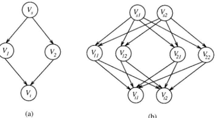
reliabil-Fig. 1. ( a ) A fork-join task graph; ( b ) its replicated graph. ity of a task running in distributed systems. Due to the
and-fork / and-join constraint of the task graph, the
tradi-tional network reliability problem [1, 3, 4, 6, 7, 11, 12 ] in the following example: Consider a simple application
is a special case of the distributed task reliability problem, modeled by an and-fork / and-join graph as shown in
Fig-where the former is known to be NP-hard for general ure 1 ( a ) . ( By convention, this task operates only if all
graphs. For the two-terminal series-parallel ( TTSP ) the modules as well as the links operate.) Suppose that
graphs, the distributed task reliability can be found in the application is implemented with an extra replication.
polynomial time using the technique developed in [13 ] . In this approach, each module receives messages not only
For the two-terminal and – or series-parallel ( AOSP ) from its predecessors in the same replica, but also from
graphs, we will show in Section 2 that their distributed the corresponding predecessors in the other replica.
Fig-task reliability can also be calculated in polynomial time ure 1 ( b ) shows one such implementation. Thus, a task
using the same technique [13 ] . In this paper, we consider finishes successfully only if there is a set of modules
a graph Hk
(Vˆ , Eˆ), named the k-replicated and–or series-which forms this application, and their associated
commu-parallel graph ( k-replicated AOSP graph or, more, simply
nication links are operational. Obviously, this application
RAOSP graph ) , which is obtained from an AOSP graph may tolerate more than one fault in each task replication,
H (V, E ) by adding ( k 0 1 ) replications to each vertex depending on the fault patterns. Figure 2 shows a few
and adding proper links between vertices. The main con-examples where the task in Figure 1 ( b ) is operational.
tribution of this paper is the design of a linear time algo-The modules and the communication links may fail
rithm to calculate the reliability of the RAOSP graph due to two main factors: software failure and hardware
Hk
(Vˆ , Eˆ), given the base AOSP graph H(V, E) and the
failure. The software failures are mainly due to the design
replication degree k . It can be shown that the RAOSP faults or implementation faults. The reliability can be
graphs are not AOSP graphs; thus, the existing polyno-increased when the software components are replicated
mial algorithm does not apply. Previously, only exponen-with the N-version programming approach [ 5 ] . The
hard-ware failures are due to either transient failures or perma- tial time algorithms, as used in general graphs, are known
1. All modules in the task graph H (V, E ) are perfectly reliable.
2. Any communication link may fail with a known proba-bility.
3. All failures are assumed to occur independently of each other.
We remind the reader that we will extend this model to consider the case of unreliable modules in Section 6.
Formally, a two-terminal AOSP graph of type k , where
k √ { L , PA, PO, S } ( which means leaf, parallel-and, parallel-or, and series, respectively ) is recursively
de-fined as follows:
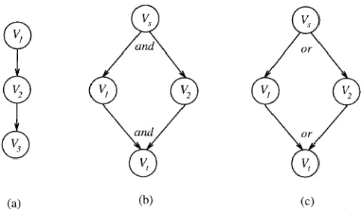
Fig. 3. ( a ) Sequential graph; ( b ) and-fork / and-join graph;
( c ) or-fork / or-join graph.
1. A single edge ( s , t ) comprises an AOSP graph of type
L with terminals s and t . The system operates if that
edge operates. to find the reliability of Hk
(Vˆ , Eˆ). In this paper, we
Let Hi be an AOSP graph with terminals si and ti for present a linear time algorithm with O ( K (ÉVÉ / ÉEÉ) )
iÅ 1, 2. complexity to compute the reliability of the graph Hk
(Vˆ ,
Eˆ ), where KÅ max { k2
22 k
, 23 k
} . 2. The graph H1ÚH2is an AOSP graph of type PAwith
The rest of the paper is organized as follows: In the terminals s and t , where the graph associated with H1
next section, the definition of AOSP graphs is given and ÚH2is the disjoint union of H1and H2, with s1
identi-the reliability evaluation for AOSP graphs is discussed. fied with s2 and t1 identified with t2, and the system
In Section 3, we define the k-replicated AOSP graph and operates if both H1and H2 operate.
its reliability. An algorithm for computing the reliability 3. The graph H
1ÛH2is an AOSP graph of type POwith of a k-replicated AOSP graph Hk
(Vˆ , Eˆ) is developed in terminals s and t , where the graph associated with H1 Section 4. The algorithm is shown to have an O ( K (ÉVÉ
Û H2 is the same as that associated with H1 Ú H2,
/ ÉEÉ) ) time complexity, where KÅmax { k222 k, 23 k} .
except that the system operates if either H1or H2
oper-A numerical example is given in Section 5. Section 6 ates. presents an extension to the model and considers the cases
4. The graph H1∗H2 is an AOSP graph of type S with
of partial replication as well as unreliable vertices.
Fi-terminals s1 and t2, where the graph associated with
nally, concluding remarks are presented.
H1∗H2is the disjoint union of H1and H2with t1
identi-fied with s2, and the system operates if both H1 and
H2operate.
2. RELIABILITY EVALUATION
We note that the TTSP graphs [13 ] can be formulated
OF AOSP GRAPHS
recursively using only the operations 1, 3, and 4 of the AOSP graphs defined previously. In other words, the class of the TTSP graphs is a subclass of the AOSP graphs. Consider a computation task graph H (V, E ) consisting of
The distributed task reliability of task H , denoted by a set of software modules V and a set of communication
R ( H ) , is defined as the probability that the task H
oper-links E , which represents message passings between
soft-ates. For example, if H contains only one edge e of type ware modules. According to the logical structures and
L , R ( H )År ( e ) , where r ( e ) is the reliability of edge e .
precedence relationship among the modules, a large class
If H consists of two AOSP graphs H1and H2, then
of task graphs can be expressed by a combination of three common types of subgraphs [ 5, 9 ] : sequential, and-fork to and-join ( AFAJ ) , and or-fork to or-join ( OFOJ ) [ see Fig. 3 ( a ) – ( c ) ] , where AFAJ and OFOJ subgraphs may
R ( H ) Å R ( H1) R ( H2) 10 ( 10R ( H1) ) ( 1 0R ( H2) ) if HÅH1ÚH2 or H ÅH1∗H2 if HÅH1Û H2. ( 1 ) consist of several sequential subgraphs in a parallel
struc-ture. In this paper, we restrict our task graphs to contain a combination of these three types of subgraphs. This type of the graph can be modeled as a two-terminal AOSP
graph. To state the model, we make the following assump- To compute R ( H ) , we first describe an AOSP graph
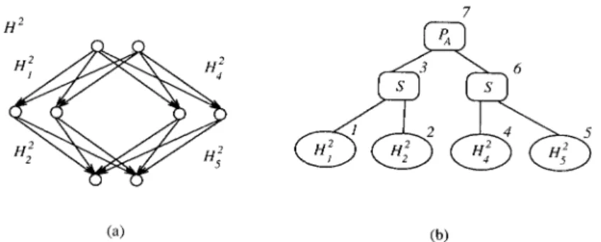
H by a binary tree structure, T ( H ) , called the parsing
tree of H . For example, Figure 4 ( b ) depicts a parsing
tree of the AOSP graph H in Figure 4 ( a ) . The nodes in the parsing tree are numbered ( at the upper right corner ) according to their postorder sequence. Each leaf node in
T ( H ) corresponds to an AOSP subgraph of type L , i.e.,
a single-edge AOSP graph in H . In Figure 4, for example,
H1Å e1, H2 Åe2, H4Å e3, and H5 Åe4. Each internal
node is labeled by S , PO, or PAaccording to the type of that AOSP subgraph. An internal node numbered x in
T ( H ) along with all of its descendant nodes induce a
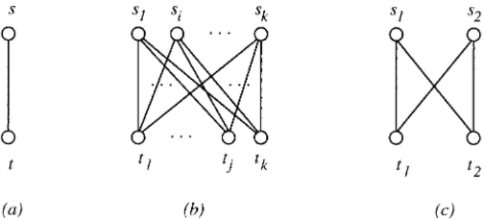
Fig. 5. ( a ) A type L AOSP graph; ( b ) the corresponding
k-subtree Txwhich also describes an AOSP subgraph Hxin
replicated RAOSP; ( c ) the 2-replicated RAOSP. H . For example, subtree T3 describes the AOSP graph
H3 Å H1∗H2, in Figure 4 ( b ) . Given the parsing tree
T ( H ) , we can obtain R ( H ) using Eq. ( 1 ) to compute the
execution; then, a replicated edge in Hk
represents a
rep-R ( Hx) level by level for every node x in the parsing tree
lica thread of the corresponding thread in H [ such as ( si, T ( H ) . For example, we first find R ( H1) and R ( H2) in
tj) , 1 ° i , j ° k , are a replica of ( s , t ) in Fig. 5 ( b ) .] Figure 4 ( b ) , where H1 Å e1 and H2 Å e2. Next, we
For clarity, we introduce the concept of ‘‘ correct value consider subtrees T3and compute R ( H3)ÅR ( H1) R ( H2) .
at terminal. ’’ Without loss of generality, the source
termi-Finally, we can determine R ( H )ÅR ( H7)ÅR ( H3ÚH6)
nal of an edge is either offered a valid input value or a
ÅR ( H3) R ( H6) .
nil value. Suppose that a valid input value is offered at Note that an AOSP graph H (V, E ) can be translated
the source terminal s of an AOSP graph H ; then, the sink into its parsing tree in O (ÉEÉ) time using the algorithm
terminal t of H is said to have a ‘‘ correct ’’ value with proposed by Valdes et al. [13 ] . In other words, R ( H ) can
respect to the valid input value if H operates.
Further-be found in O (ÉEÉ) time.
more, the sink terminal t has a n il value if either the source terminal is offered as a valid input value but H fails to operate or the source is offered a nil value regardless of
3. TASKS WITH REPLICATION
the operation of H .*
Consider a k-replicated AOSP graph Hk
. We first no-To increase the reliability of a task, we replicate the
mod-tice that it has k source terminals and k sink terminals. ules and the message passing links of the task. The
k-Without loss of generality, we assume that those source
replicated task graph Hk
(Vˆ , Eˆ) of H(V, E) is created by
terminals of Hk
which are offered valid input have the replicating each vertex in V ( k01 ) times and letting the
same input value. It is obvious that whether a sink termi-edges in Hk
be established in such a way that each vertex
nal of Hk
has a correct output depends not only on which is not only descendant of its predecessors in the same
source terminals of Hk
are offered valid input values but replica, but is also descendant to the corresponding
prede-also on the execution of Hk
. Let S and T be the sets of cessors in the other replicas. For example, Figure 5 ( b )
source and sink terminals of Hk
, respectively. Let A be shows a k-replicated task graph created from an AOSP
the set of source terminals offered with the same valid graph of type L in Figure 5 ( a ) .
input value and B be the set of sink terminals with correct Imagine that each edge in H represents a thread of
outputs; A ⊆ S , B ⊆ T . Hk
is said to operate w.r.t. ( A ,
B ) if∀tj√B , tjhas a correct value and ∀t*j √T"B , t*j has nil value, given that ∀si √ A , si are offered with a valid input value and other source terminals are offered a nil value. Now, we are ready to formally define the k-replicated AOSP graph:
1. ( L ) : A k-replicated AOSP structure of type L consists of a set of k source terminals, SÅ{ s1, . . . , sk} , a set of k sink terminals, TÅ { t1, . . . , tk} , and k
2
edges, ( si, tj) ,∀i , j . Let A⊆S , B ⊆T . The system operates w.r.t. ( A , B ) iff ∀tj √ B ,∃si √A , such that ( si, tj)
Fig. 4. ( a ) A fork-join AOSP graph; ( b ) the corresponding
R ( Hk )Å Pr { < B⊆T,Bx0/ ESB( H k ) } , operates and∀t*j √ T"B , "∃si √ A such that ( si, t*j)
operates. Å
∑
M xB⊆T pSB( H k ) . ( 2 ) Let Hkibe a k-replicated AOSP graph with terminals set Si and Ti, and let Ai ⊆ Si, Bi ⊆ Ti, for iÅ1, 2. 2. ( PA) : The graph H
k
1 Ú H
k
2 is a k-replicated AOSP A straightforward way to compute R ( Hk) is to enumerate
graph of type PA with terminals set S and T , where the execution outcomes of all the edges in Hk( Eˆ , Vˆ ), the graph associated with Hk
1 Ú H
k
2 is the disjoint where ÉEˆÉ Å k2rÉEÉ and set E is an edge set in H .
union of Hk
1and Hk2, with S1identified with S2( i.e., However, this method takes O ( 2k
2ÉE É
) . In next section,
s1i √S1 identified with s2i √S2, 1 ° i ° k ) and T1 a linear time algorithm for computing R ( Hk) will be
pre-identified with T2. Furthermore, S Å S1 Å S2 and T sented.
ÅT1ÅT2. Suppose that A⊆S and B⊆T . The system
operates w.r.t. ( A , B ) iff Hk
1operates w.r.t. ( A , B1) ,
Hk
2operates w.r.t. ( A , B2) , and B1> B2ÅB . 4. RELIABILITY EVALUATION OF RAOSP
GRAPHS
3. ( PO) : The graph Hk1 Û Hk2 is a k-replicated AOSP
graph of type PO with terminals set S and T , where
In this section, we present an algorithm to compute the the graph associated with Hk
1 Û Hk2 is the disjoint
reliability of a k-replicated task Hk
(Vˆ , Eˆ) in O(KÉEÉ)
union of Hk
1and H
k
2, with S1identified with S2and T1
time. Note that KÅmax { k2
22 k
, 23 k
} . We first consider identified with T2. Let S Å S1 Å S2, and T Å T1
the k-replicated task graph of type L . [ See Fig. 5 ( b ) for
Å T2. Suppose that A ⊆ S and B ⊆ T . The system
an example of Hk
.] Suppose that A ⊆ S and B⊆T . For
operates w.r.t. ( A , B ) iff Hk
1operates w.r.t. ( A , B1) ,
any t √B , the probability that at least one edge ( s , t ) , Hk
2operates w.r.t. ( A , B2) , and B1< B2ÅB .
s√A , operates is ( 10∏s√ APr[ ( s , t ) fails ] ) . Thus, for 4. ( S ) : The graph Hk
1∗H
k
2is a k-replicated AOSP graph
the k-replicated AOSP graph Hk
of type L , we have of type S with terminals sets SÅS1and TÅT2, where
the graph associated with Hk
1∗H
k
2is the disjoint union
( L ) : pAB( H k )Å{
∏
t√ B ( 10∏
s√ A Pr [ ( s , t ) fails ] ) } of Hk1and Hk2with T1identified with S2. Suppose that
A ⊆ S and B ⊆ T . The system operates w.r.t. ( A , B )
1{
∏
t√ T "B∏
s√ A Pr [ ( s , t ) fails ] } . ( 3 ) iff Hk 1operates w.r.t. ( A , B1) , H2koperates w.r.t. ( A2, B ) , and B1ÅA2.For convenience, let M denote the matrix of pAB( Hk) , so that M Å [ pAB( Hk) ]A⊆S,B⊆T with dimension 2k 1 2k. Let EAB( Hk) be a probability event that Hkoperates w.r.t.
terminal sets ( A , B ) . We denote pAB( Hk) Å Pr { EAB For example, a 2-replicated AOSP graph of type L , H2(Vˆ , Eˆ ) is obtained from edge (s, t), where Vˆ Å { s1, s2, t1,
( Hk
) } . We notice that for any set A⊆ S , (B⊆TpAB( Hk)
Å1. Given that all the source terminals are offered with t2} and Eˆ Å { ( s1, t1) , ( s1, t2) , ( s2, t1) , ( s2, t2) } . Let
probabilities r1, r2, r3, and r4 ( rV1, rV2, rV3, and rV4) be the
the valid input value initially, i.e., AÅS , the reliability
of Hk
is the same as the probability that at least one sink reliabilities ( unreliabilities ) of edges ( s1, t1) , ( s2, t1) , ( s1,
t2) , and ( s2, t2) , respectively. Then, the matrix M of H 2
terminal has a correct value. Thus, the reliability of Hk
is defined as is MÅ p{s1,s2} , {t1,t2}( H2) p{s1,s2} , {t1}( H2) p{s1,s2} , {t2}( H2) p{s1,s2} , {}( H2) p{s1} , {t1,t2}( H 2 ) p{s1} , {t1}( H 2 ) p{s1} , {t2}( H 2 ) p{s1} , {}( H 2 ) p{s2} , {t1,t2}( H 2 ) p{s2} , {t1}( H 2 ) p{s2} , {t2}( H 2 ) p{s2} , {}( H 2 ) p{} , {t1,t2}( H 2 ) p{} , {t1}( H 2 ) p{} , {t2}( H 2 ) p{} , {}( H 2 ) Å ( 1 0rV1rV2) ( 1 0rV3rV4) ( 1 0rV1rV2) rV3rV4 ( 10 rV3rV4) rV1rV2 rV1rV2rV3rV4 r1r3 r1rV3 r3rV1 rV1rV3 r2r4 r2rV4 r4rV2 rV2rV4 0 0 0 1 , ( 4 )
where {} represents the null set. ( PO) : pAB( H k 1ÛH k 2) Next, we consider Hk Å Hk 1Ú H k 2. By definition, the Å
∑
B1⊆T1,B2⊆T2 s .t .B1<B2ÅB pAB1( H k 1)rpAB2( H k 2) . ( 7 ) terminal sets S and T of Hkare given as SÅS1ÅS2and
TÅT1ÅT2. Suppose that A⊆S , B1⊆T1, and B2⊆ T2;
then, the event [ EAB1( H k
1) ] Ú [ EAB2( H k
2) ] implies the
For example, let H2
i be a 2-replicated AOSP graph event EAB( H
k
1Ú H
k
2) if B1> B2 ÅB . Thus,
with terminal sets Siand Ti for iÅ1, 2, respectively. Let S1Å { s11, s12} , S2Å{ s21, s22} , T1 Å{ t11, t12} , and T2
EAB( Hk1ÚHk2)Å <
B1⊆T1,B2⊆T2 s .t .B1>B2ÅB
{ EAB1( Hk1) ÚEAB2( Hk2) } , Å{ t
21, t22} . Let ( H21 Û H22) be the 2-replicated AOSP
graph obtained from H2 1 and H
2
2with terminals ( s1, s2)
and ( t1, t2) . Note that ( s1, s2) Å ( s11, s12) Å ( s21, s22)
and ( t1, t2) Å ( t11, t12) Å ( t21, t22) . Then, for any A
i.e.: ⊆{ s1, s2} , ( PA) : pAB( Hk1ÚHk2) pA , {}( H12ÛH22)Å pA , {}( H21) pA , {}( H22) , Å
∑
B1⊆T1,B2⊆T2 s .t .B1>B2ÅB pAB1( H k 1)rpAB2( H k 2) . ( 5 ) pA , {t1}( H 2 1ÛH 2 2) Å pA , {}( H 2 1) pA , {t21}( H 2 2) /pA , {t11}( H 2 1) pA , {}( H 2 2) /pA , {t11}( H 2 1) pA , {t21}( H 2 2) ,For example, let H2
i be a 2-replicated AOSP graph
with terminal sets Siand Ti for iÅ1, 2, respectively. Let pA , {t 2}( H 2 1ÛH 2 2) Å pA , {}( H 2 1) pA , {t22}( H 2 2) ( 8 ) S1Å { s11, s12} , S2Å{ s21, s22} , T1 Å{ t11, t12} , and T2 /pA , {t12}( H 2 1) pA , {}( H 2 2)
Å{ t21, t22} . Let ( H21 Ú H22) be the 2-replicated AOSP
graph obtained from H2
1 and H22with terminals ( s1, s2)
/pA , {t12}( H
2
1) pA , {t22}( H
2 2) ,
and ( t1, t2) . Note that ( s1, s2) Å ( s11, s12) Å( s21, s22)
and ( t1, t2) Å( t11, t12) Å( t21, t22) . pA , {t
1,t2}( H
2
1Û H22)Å10[ pA , {}( H21ÛH22)
By Eq. ( 5 ) , for any A⊆ { s1, s2} , we have
/pA , {t1}( H 2 1ÛH22) pA , {t1,t2}( H 2 1ÚH22)Å pA , {t11,t12}( H 2 1) pA , {t21,t22}( H 2 2) , / pA , {t2}( H 2 1ÛH22) ] . pA , {t1}( H 2 1ÚH22) Å pA , {t11,t12}( H 2 1) pA , {t21}( H 2 2) Finally, we consider Hk Å Hk 1∗H k 2. By definition of
the k-replicated AOSP graph of type S , the event
/pA , {t11}( H 2 1) pA , {t21,t22}( H 2 2) [ EAB1( H k 1)> EA2B( H k
2) ] implies the event EAB( H k 1∗H k 2) if B1ÅA2. So, we have /pA , {t11}( H 2 1) pA , {t21}( H 2 2) , EAB( Hk1∗Hk2) Å < B1⊆T1,A2⊆S2 s .t .B1ÅA2 [ EAB1( H k 1) ÚEA2B( H k 2) ] . pA , {t2}( H21ÚH22) Å pA , {t11,t12}( H21) pA , {t22}( H22) ( 6 ) /pA , {t12}( H 2 1) pA , {t21,t22}( H 2 2) Therefore, /pA , {t12}( H 2 1) pA , {t22}( H 2 2) , ( PS) : pAB( Hk1∗Hk2) pA , {}( H 2 1 ÚH 2 2)Å10[ pA , {t1,t2}( H 2 1ÚH 2 2) Å
∑
B1⊆T1,A2⊆S2 s .t .B1ÅA2 pAB1( H k 1)rpA2B( H k 2) . ( 9 ) /pA , {t1}( H 2 1ÚH22) / pA , {t2}( H21ÚH22) ] .For example, let H2
i be a 2-replicated AOSP graph with terminal sets Siand Ti for iÅ1, 2, respectively. Let Thus, a 22
122
matrix MÅ[ pAB( H
2
) ]A⊆S,B⊆Tfor graph S1Å { s11, s12} , S2Å{ s21, s22} , T1 Å{ t11, t12} , and T2 H2
1Ú H22can be obtained using the above equations. Å{ t21, t22} . Let ( H21∗H22) be the 2-replicated AOSP
ob-tained from H2
1 and H22 with terminals ( s1, s2) and ( t1,
Similarly, let HkÅ Hk
1Û Hk2with terminal sets S and
T , where SÅS1 ÅS2and T ÅT1Å T2. Then, for any t2) . Note that ( s1, s2)Å( s11, s12) , ( t11, t12)Å( s21, s22) ,
and ( t1, t2) Å( t21, t22) . Then,
Fig. 6. ( a ) A numerical example; ( b ) its corresponding parsing tree.
It is known that Step 1 takes O (ÉEÉ) [13 ] . In Step 2,
pAB( H 2 1∗H 2 2)ÅpA , {t11,t12}( H 2 1) p{s21,s22} ,B( H 2 2) if Hk
x is of type L , it takes O ( k2) time to compute each
/pA , {t11}( H21) p{s21} ,B( H22)
( 10 ) entry in matrix Mx and, thus, O ( k22k) time in total for matrix Mx. If H k x is of type PAor PO, it takes O ( 2 kr 2k ) /pA , {t12}( H 2 1) p{s22} ,B( H 2 2)
to compute each row in matrix Mxand, thus, O ( 2
3 k ) time /pA , {}( H21) p{} ,B( H22) . for matrix Mx. If H k x is of type S ( say H k x Å H k y∗H k z) , matrix Mx is obtained from multiplying My by Mz and, Let Hk
(Vˆ , Eˆ) be the k-replicated AOSP graph derived thus, it takes O ( 23 k
) time to compute matrix Mx. Thus, from H (V, E ) . Since Hk
is derived from H , the structure the total time in Step 2 is O ( max { k2
22 kÉ
EÉ, 23 kÉEÉ} ) .
of the parsing tree of H , T ( H ) , is equivalent to the struc- Hence the time complexity of Algorithm 1 is O ( KÉEÉ) ,
ture of the parsing tree of Hk , T ( Hk ) , i.e., T ( H )áT ( Hk ) . where KÅmax { k2 22 k , 23 k } . The only difference is that the leaf nodes in T ( H ) are
type L AOSP graphs, whereas the leaf nodes in T ( Hk ) are type L RAOSP graphs with degree k . Therefore,
T ( Hk
) can be obtained by applying the algorithm [13 ] to 5. A NUMERICAL EXAMPLE its base AOSP graph H .
As discussed, each leaf node with the postorder se- We illustrate the calculation of the distributed task relia-quence x in T ( Hk
) corresponds to an RAOSP subgraph bility in this section through an example: Consider a 2-of type L , denoted as Hk
x. Every internal node x is labeled replicated AOSP graph H2
as shown in Figure 6 ( a ) , by S , PO, or PA according to the type of that RAOSP which is generated from the AOSP graph in Figure 4 ( a ) . subgraph. Similar to the T ( H ) , every internal node x in It is readily seen that H2
Å H2 7 Å ( H 2 1∗H 2 2) T ( Hk
) , along with all its descendant nodes, induces a Ú ( H2
4∗H25) , where H21, H22, H24, and H25are 2-replicated
subtree Txwhich describes a k-replicated AOSP subgraph AOSP subgraphs of type L . [ See Fig. 5 ( c ) for k Å 2.] Hk
xin H k
. Therefore, Mrfor root node r can be determined In analogy to the parsing tree of H in Figure 4 ( b ) , the by computing the Mx level by level for every node x in parsing tree for H2
is given in Figure 6 ( b ) . the parsing tree T ( Hk
) using Eqs. ( 3 ) , ( 5 ) , ( 7 ) , and ( 9 ) .
Suppose that the reliability of each link in H2
i is ri, Finally, R ( Hk
)Å(M xB⊆TpSB( H k
) is emerged in the first
for iÅ 1, 2, 4, 5. Let r1 Å0.9, r2 Å0.8, r4 Å0.7, and
row of matrix Mr. r
5Å 0.7. To calculate R ( H2) , we first calculate the Mi We now present the algorithm:
matrices for H2
i, i Å1, 2, 4, 5. From Eq. ( 4 ) , we have
Algorithm 1
STEP 1. Find the parsing tree of the graph Hk, denoted
M1Å 0.9801 0.0099 0.0099 0.0001 0.81 0.09 0.09 0.01 0.81 0.09 0.09 0.01 0 0 0 1 , as T ( Hk
) , by applying Valdes’ algorithm to H [13 ] . STEP 2. Evaluate the matrix Mx for each node x in the
parsing tree T ( Hk
) by postorder traversal.
STEP 3. Compute R ( Hk) Å (⊆xB⊆T pSB( Hk) , where the
M2Å 0.9216 0.0384 0.0384 0.0016 0.64 0.16 0.16 0.04 0.64 0.16 0.16 0.04 0 0 0 1 ,
terms pSB( Hk) can be found in the first row of matrix Mrat root node r in T ( Hk) .
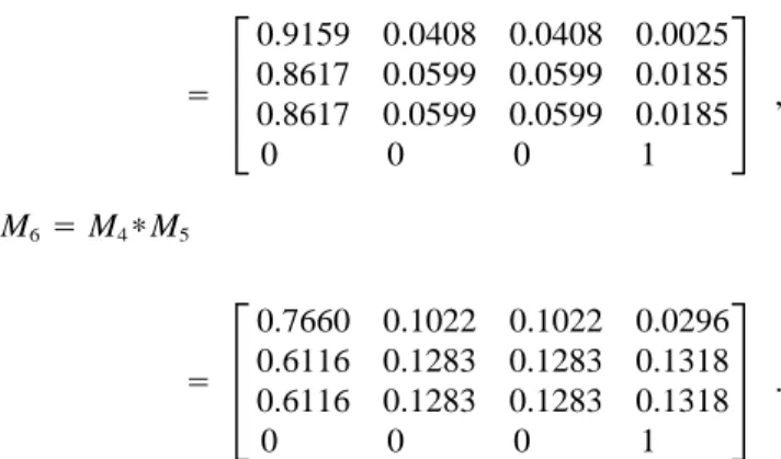
M3ÅM1∗M2 M4Å 0.8281 0.0819 0.0819 0.0081 0.49 0.21 0.21 0.09 0.49 0.21 0.21 0.09 0 0 0 1 , Å 0.9159 0.0408 0.0408 0.0025 0.8617 0.0599 0.0599 0.0185 0.8617 0.0599 0.0599 0.0185 0 0 0 1 , M6ÅM4∗M5 M5Å 0.8281 0.0819 0.0819 0.0081 0.49 0.21 0.21 0.09 0.49 0.21 0.21 0.09 0 0 0 1 . Å 0.7660 0.1022 0.1022 0.0296 0.6116 0.1283 0.1283 0.1318 0.6116 0.1283 0.1283 0.1318 0 0 0 1 . Next, we consider the subgraphs ( H2
1∗H 2 2) and
( H2
4∗H25) , i.e., the subtrees rooted at nodes 3 and 6 in Finally, we consider H2. Given M3and M6, we obtain
Figure 6 ( b ) . Applying Eq. ( 10 ) , we have the matrix MÅM7for H2using Eq. ( 6 ) . Thus,
MÅM7Å p{s ,s= } , {t ,t = }( H2) p{s ,s= } , {t }( H2) p{s ,s= } , {t = }( H2) p{s ,s= } , {}( H2) p{s } , {t ,t= }( H2) p{s } , {t }( H 2 ) p{s } , {t= }( H2) p{s } , {}( H 2 ) p{s= } , {t ,t = }( H 2 ) p{s= } , {t }( H 2 ) p{s= } , {t = }( H 2 ) p{s= } , {}( H 2 ) p{} , {t ,t= }( H2) p{} , {t }( H2) p{} , {t= }( H2) p{} , {}( H2) Å 0.7016 0.1290 0.1290 0.0404 0.5270 0.1549 0.1549 0.1632 0.5270 0.1549 0.1549 0.1632 0 0 0 1 .
Finally, the reliability of H2
can be obtained by Eq. ( 2 ) : graph of type L and is fully replicated. The RAOSP graph
H*k
Å ( VV , EV) is partially replicated if VV ⊆ Vˆ and/or EV
⊆Eˆ . To compute R(Hk
) , we first add those unreplicated
R ( H2 )Å Pr { < B⊆T,Bx0/ ESB( H 2 ) }Å
∑
0/ xB⊆T pSB( H 2 )vertices and edges ( vertices and edges that would have been in a fully replicated Hk
) into VV and EV and simply
Å p{s ,s= } , {t ,t = }( H 2 )/p{s ,s= } , {t }( H 2 ) /p{s ,s= } , {t = }( H 2 )
set the reliability of those edges to 0, i.e., Pr { ( si, tj)
Å0.7016/0.1290/0.1290Å0.9596. operates }Å0,∀( si, tj)√Eˆ Ú( si, tj)√/ EV . After adding
those edges, H*k
becomes fully replicated and R ( H*k ) can be obtained via Eq. ( 3 ) . Now, we summarize the
6. FURTHER DISCUSSION reliability analysis of the general RAOSP graph Hk
with partial replication; we first find its parsing tree using the In Section 4, we assumed that a k-replicated AOSP graph same algorithm in [13 ] . Then, we convert each RAOSP is fully replicated, i.e., each vertex is replicated exactly graph of type L in Hk
into a fully replicated RAOSP graph ( k01 ) times and each edge is replicated ( k01 )2
times. of type L as shown above. Then, we apply Steps 2 and Furthermore, we assumed that all vertices are perfectly 3 in Algorithm 1 to obtain the reliability of Hk
.
reliable. In this section, we first extend our model to We next consider the RAOSP graphs with unreliable consider those cases where vertices and edges are partially vertices. We begin the discussion with the AOSP graphs. replicated. Later on, we present a solution method to the To incorporate the unreliable vertices into our graph problem that both vertices and edges can fail. model, for each vertex ( or terminal ) t in an AOSP graph, To calculate the reliability of partially replicated we replace it by an edge ( t , t*) and assign the reliability RAOSP graph, we first convert such a graph into a fully of that edge to be the failure probability of that vertex. replicated RAOSP graph, then calculate its reliability us- [ See Fig. 7 ( b ) as an example.] Similarly, to consider the unreliable vertices ( or terminals ) in an RAOSP graph Hk
, ing Algorithm 1. Suppose that HkÅ
graph problems there may also exist polynomitime al-gorithms for RAOSP graphs provided there exist polyno-mial-time algorithms for AOSP graphs.
REFERENCES
[1] A. Agrawal and R. E. Barlow, A survey of network relia-bility and domination theory. Oper. Res. 32 ( 1984 ) 478 – 492.
Fig. 7. ( a ) A single vertex; ( b ) its AOSP equivalent; ( c ) a
[ 2 ] P. A. Alsberg and J. D. Day, A principle for resilient
vertex and its replica; ( d ) its RAOSP equivalent.
sharing of distributed resources. Proceedings of the 2nd International Conference on Software Engineering ( Oct. 1976 ) 562 – 570.
we can also replace each terminal in Hk
by an edge. As
[ 3 ] S. Arnborg and A. Proskuronski, On network reliability.
shown in Figure 7 ( c ) and ( d ) , it is a terminal after being
Discr. Appl. Math. 23 ( 1 ) ( 1989 ) 11 – 24.
replicated once and each terminal being replaced by an
[ 4 ] M. O. Ball, Computational complexity of network
relia-edge. We notice that this structure is an RAOSP graph
bility analysis: An overview. IEEE Trans. Reliab.
R-of type L with partial replication, and, thus, its reliability
35 ( 3 ) ( 1986 ) 230 – 239. can be obtained using the method presented in the
previ-[ 5 ] W. W. Chu and K. K. Leung, Module replication and
ous section.
assignment for real-time distributed processing systems. Proceed. IEEE 75 ( 1987 ) 547 – 562.
[ 6 ] C. J. Colbourn, The Combinatorics of Network Reliabil-7. CONCLUSIONS
ity. Oxford University Press, New York ( 1987 ) . [ 7 ] S. Hariri and C. S. Raghavendra, Syrel: A symbolic
re-This paper has focused on the design of an efficient
algo-liability algorithm based on path and cutset methods.
rithm to predict the reliability of tasks characterized by
IEEE Trans. Comput. C-36 ( 1987 ) 1224 – 1232.
replicated and – or series-parallel ( AOSP ) graphs. A
k-[ 8 ] S.-T. Levi, S. Tripathi, S. Carson, and A. Agrawala, The
replicated AOSP graph is derived from an AOSP graph
maruti hard real-time operating system. ACM Oper. Syst.
with vertex and edge replications. Conventional
algo-Rev. 23 ( 1989 ) 90 – 105.
rithms may apply to compute the reliability of a
k-repli-[ 9 ] V. W. Mak and S. F. Lundstrom, Predicting performance
cated AOSP graph. However, these algorithms take expo- of parallel computations. IEEE Trans. Parallel Distrib. nential time in the number of edges. We have presented Syst. 1 ( 1990 ) 257 – 270.
an algorithm with time complexity O ( K (ÉVÉ / ÉEÉ) ) ,
[10 ] D. Powell, Delta-4: Overall System Specification. The
where K Å max { k2
22 k
, 23 k
} andÉVÉ and ÉEÉ are the
Delta-4 Project Consortium ( 1988 ) .
number of vertices and edges, respectively, in its corre- [11] C. S. Raghavendra, V. K. Prasanna, J. Kumar, and S. sponding AOSP graph. In real-life applications, the k is Hariri, Reliability analysis in distributed systems. IEEE typically small whereasÉVÉ/ ÉEÉis much larger ; thus,
Trans. Comput. C-37 ( 1988 ) 352 – 358.
our algorithm is a significant improvement over the tradi- [12 ] A. Satyanarayana and A. Prabhakar, New topological
tional approaches. formula and rapid algorithm for reliability analysis of
Many graph-related problems are NP-complete for complex networks. IEEE Trans. Reliab. R-27 ( 2 ) ( 1979 )
general graphs but can be solved in polynomial-time for 82 – 100.
AOSP graphs. In this paper, we have shown that the [13 ] J. Valdes, R. Tarjan, and E. L. Lawler, The recognition
distributed task reliability problem can also be solved in of series parallel digraphs. SIAM J. Comput. 11 ( 1982 ) 298 – 313.