國立臺灣大學生農學院森林環境暨資源學研究所 博士論文
School of Forestry and Resource Conservation College of Bio-resources and Agriculture
National Taiwan University Doctoral Dissertation
應用遙測技術於臺灣北部地區水文循環之研究
Study on the Hydrologic Cycle of the Northern Taiwan Using Remote Sensing Techniques
吳治達 Chih-Da Wu
指導教授:羅漢強 博士 鄭祈全 博士 Advisor: Hann-Chung Lo, Ph.D.
Chi-Chuan Cheng, Ph.D.
中華民國 99 年 4 月
April, 2010
謝 誌
光陰荏苒,自研究所起算,轉瞬間在台大已度過了七年的時光,隨著求學
生涯即將暫告一段落,心中湧現的,是對於過程中眾人的支持無限的感恩。
本論文承蒙恩師 羅漢強教授及 鄭祈全教授之引導啟發,求學期間兩位恩 師不時指導學生正確的方向,並於研究架構與內容惠賜卓見、逐字匡正,論文始 能順利付梓,內心感恩之情,難以言喻,謹誌卷首,以申謝忱。
論文初稿,復蒙屏東科技大學陳朝圳副校長、銘傳大學觀光學院陳永寬院 長、嘉義大學森林暨自然資源學研究所林金樹主任、政治大學地政學研究所詹進 發副教授、文化大學森林暨自然保育學系許立達副教授詳予審閱口試,匡正謬 誤,惠賜卓見,使本文更臻完善,衷心感謝。
衷心感謝恩師嘉義大學森林暨自然資源學研究所 林金樹主任及 林喻東 老師不斷之教導與鼓勵,引領學生進入森林經營與遙感探測之研究領域,學生始 得完成碩士及博士學業,老師栽培之苦心,學生永銘在心。
感謝美國愛達荷州立大學研究發展中心 Rick Allen 博士於程式撰寫上之協 助;美國國家職業安全衛生中心 Lynda M. Ewers 博士在論文文法及用詞上之逐 字匡正;屏東科技大學森林系陳朝圳老師及鐘玉龍老師於分析程式及材料上之提 供;台灣大學生物環境系統工程學系童慶斌老師於分析程式上之提供;內政部國 土測繪中心於國土利用調查資料之提供,使論文能順利完成,謹致上最誠摯之謝 意。
研究期間,感謝焦國模老師及陳永寬老師在航、遙測方面的啟蒙,以及日常 生活及為人處世方面之諸多指導;羅漢強老師及鄭祈全老師於課業上之指點;政 治大學詹進發老師於研究架構上之指導;彰化師範大學王素芬老師於集水區生態 學方面多所指正;師母范秀蘭女士在各方面的照顧及協助;葉堃生學長、鄧淑萍 學姐、吳耀楠學長、學妹施瑩瑄及陳奐閔之多方鼓勵;同窗好友,加拿大英屬哥
倫比亞大學莊永忠博士後研究員在求學期間的同甘共苦,相互勉勵;政治大學地 政學系遙測實驗室的彥廷、阿瑪、郁晴、幸宜、奧莉薇、安勤、清智、曉彤,你 們的幫忙及搞笑,均是難以忘懷之回憶,在此致上無盡的謝意。
感謝全家人及父母多年來的支持,使我得以在學術研究上全力衝刺,無後顧 之憂;此外,摯友慧如多年來不離不棄,默默支持,一路相伴,更是我前進的動 力,沒有妳的體諒、包容,相信這七年的生活將是很不一樣的光景。
最後,謹以此文獻給曾經幫助過我的所有人。
吳治達 謹識於
台灣大學森林環境暨資源學研究所森林攝影測量研究室 中華民國 99 年 4 月
中文摘要
環境變遷與集水區水文循環之間的關係已成為環境規劃的重要課題。國內外 已有許多專家學者結合大氣環流模式 (General Circulation Models, GCMs) 與
GWLF 河川流量模式 (Generalized Watershed Loading Functions,GWLF),探討氣候 變遷對集水區水資源的衝擊效應。但大部份的研究除受限於大尺度地表蒸發散量 的調查不易之外,在蒸發散覆蓋係數 (Evapotranspiration Cover Coefficient, CV) 之 設定方面,亦大多根據 GWLF 手冊中所列之參考值進行設定。然真實地表之土地 使用類別甚為複雜,如僅依手冊中之參考值進行參數設定,可能會影響分析結果 之正確性。此外,土地使用型態和蒸發散量的逐年變化,亦會影響集水區之未來 水文狀態,而傳統的流量模擬研究甚少針對此兩項因子之影響效應加以探討。
有鑑於此,本研究以台灣北部地區為試區,旨在利用遙測技術推估真實地表 的蒸發散量與 CV 值,以提昇流量模擬之正確性,進而結合 SEBAL 模式 (Surface Energy Balance Algorithm for Land, SEBAL)、CGCM1 大氣環流模式 (The First Version of the Canadian Global Coupled Model; CGCM1) 與 Markov 模式,模擬未來 土地使用型及蒸發散量的變化,並分析其對未來流量模擬之影響,最後再綜合氣 候、土地使用及蒸發散量等環境變遷因子,進一步評估台灣北部地區未來水文循 環可能遭受之衝擊效應。研究方法首先利用遙測混合式分類方法進行台灣北部地 區之大地資源衛星(Landsat-5)的土地使用分類,並配合數值地形模型(Digital Terrain
Model, DTM)與 SEBAL 能量平衡模式,先計算與蒸發散量有關之 16 項環境參數,
再推估地表蒸發散量,並比較各土地使用型之蒸發散量,過程中為評估空間尺度 和生態分類系統二因子對環境參數之影響,乃選定兩種空間尺度 (台灣北部地區及 其轄內的 7 個集水區)和兩種生態分類系統 (12 個地理氣候分區及 7 個集水區),透 過多變量逐步判別分析方法,探討該二因子對環境參數之影響效應;其次,在利 用 SEBAL 模式計算蒸發散量和應用遙測方法推估 CV 值之後,進而應用 GWLF 模式模擬淡水河集水區之河川流量,目的除了驗證流量模式之適用性之外,並評 估傳統查表方法和遙測方法所推估之 CV 的流量模擬差異;最後,以兩期土地使用 資料為基礎,整合 Markov 模式與 CGCM1 模式,預測未來短、中、長期之土地使 用變遷、並推估其 CV,再經由 GWLF 之流量分析,分析土地變遷及蒸發散變化 對於未來河川流量之影響,進而評估北台灣地區水文系統可能遭遇到的衝擊效應。
研究結果指出,北台灣地區經混合式影像分類後,計分為森林、建地、水體、
耕作農地、休耕農地、雲及陰影 7 類土地使用型,其整體分類準確度經檢核區檢 定後為 89.00%;在土地使用型之蒸發散量方面,以森林最大 (一月:0.723cm;七 月:0.395cm),建地為最小 (一月:0.220cm;七月:0.088cm);在空間尺度和生態 分類系統對環境參數之影響分析方面顯示,使用不同生態分類系統和空間尺度來 區分 5 種土地使用型 (森林、建地、水體、耕作農地及休耕農地) 所需要的環境參 數與參數數目皆不盡相同,但常態化差異植生指標與地表熱紅外光放射率兩項參 數,不管在那一種生態分類系統,均為重要的判別參數;在利用蒸發散量和土地
使用兩因子模擬河川流量之結果顯示,利用遙測推估之 CV 值(濕季:1.245;乾季:
0.851) 與查表所得之 CV 值 (濕季:0.842; 乾季:0.717) 確實有差異。若透過流量 站的觀測資料,並結合廻歸分析進行模式檢核時發現,利用遙測推估值所模擬之 流量與觀測流量之間的相關係數為 0.877,較查表值之 0.853 為佳;至於未來土地 使用變遷與蒸發散量變化之預測結果指出,建地面積由 1995 年的 13.36%和 2002 年的 14.05%,增加為 2030 年的 38.91%,2058 年的 52.13%及 2086 年的 62.36%,
此現象會造成未來短期、中期及長期之 CV 值呈逐漸下降的趨勢,而在 GWLF 模 式之流量分析結果指出,不管是未來短期、中期或長期的月平均流量、年總流量 及年平均流量,考慮未來土地使用變遷與蒸發散量變化兩項因子所模擬的流量均 較未考慮的流量值低;最後,未來集水區水資源衝擊評估結果指出,由於都市擴 張、蒸發散量減少及氣候變遷等因子之綜合作用,將造成台灣北部地區河川流量 之上升。
綜合上述結果可知,整合 SEBAL、CGCM1 與 Markov 模式模擬土地使用變遷 及蒸發散量變化,進而推估未來集水區之河川流量及評估區域水資源之衝擊效 應,確實為一有效、可行的方法。由於台灣北部地區為經濟商業之核心區域,無 論在工商業發展及水資源供給方面均占有相當重要的地位,因此相關單位應重視 此課題,並及早研擬因應策略。
【關鍵詞】:遙測技術,水文循環,SEBAL 模式,GWLF 模式,CGCM1 大氣環流
模式,蒸發散覆蓋係數,流量模擬。
ABSTRACT
Watershed hydrology, especially stream flow, is expected to be highly sensitive to the influences of global climate change. Traditional studies have integrated the General Circulation Models (GCMs) with the Generalized Watershed Loading Function (GWLF) model to estimate stream flow rates. However, using these models in the context of a transitioning climate and on a large spatial is problematic, particularly for the estimation of two important parameters, evapotranspiration (ET) and cover coefficient (CV).
This study focuses on an integrated analysis of the hydrological cycle using remote sensing techniques to estimate the ET and the CV. Furthermore, we improved on older studies by integrating the Surface Energy Balance Algorithm for Land (SEBAL) model, the First Version of the Canadian Global Coupled Model (CGCM1), and the Markov model which allows us to predict land-use and ET change. The results were applied to assess the future impacts of global warming on hydrological cycles of northern Taiwan. Our methods include applying hybrid image classification to generate the land-use maps of the northern Taiwan using Landsat-5 images; using digital terrain model (DTM) and the SEBAL model to calculate 16 environmental parameters relevant to ET. We then compared the differences among different land-use types; (1) investigating the effects of two ecosystem classification systems (i.e., watershed division method and geographic climate method) at various spatial scales on
environmental parameters using stepwise discriminant analysis; (2) comparing stream flow simulations according to the GWLF model with two CV values derived from remote sensing and traditional methods; (3) integrating the Markov model and the CGCM1 model to predict future land-use and CV parameters for evaluating the effect of land-use change and ET change; and (4) finally, assessing the future impacts on hydrological cycle of the northern Taiwan.
The results indicated that the study area was classified into seven land types (i.e., forest, building, water, farmland, fallow farmland, cloud-covered, and shadow-covered) with 89.09% classification accuracy. These last two land types could not be analyzed further. A comparison of daily ET values among different land-use types revealed differences. In this study, forest ET is the largest (January: 0.723cm; November:
0.395cm) while building is the smallest (January: 0.220cm; November: 0.088cm). These differences contrive to exist for ecosystem classification systems at various scales, but depend on the selected environmental parameters and the number of parameters included in the model. Two parameters, a normalized difference vegetation index and an emissivity are important factors for discriminating land types. On the aspect of land-use and ET effects on hydrological simulations, the stream flows simulated by two estimated CVs were different. The stream flow simulation using the remote sensing approach (wet season: 1.245; dry season: 0.851) presented more accurate hydrological
characteristics than the traditional approach (wet season: 0.842; dry season: 0.717).
Meanwhile, according to the result of regression analysis, the flow simulation using RSCV (remote sensing based CV; regression coefficient = 0.877) would represent truer
flow characteristics than the use of REFCV (reference CV; regression coefficient = 0.853). In the prediction of future land-use and ET, due to the increase of building area from 13.36% in 1995 and 14.05% in 2002 to 38.91% in 2030, 52.13% in 2052, and 62.36% in 2086, the predicated CV values for next three periods display a decreasing trend no matter under which climatic change storyline. In addition, land-use and ET change indeed affect the predicted stream flows. The predicted flows with consideration of these two factors were lower than those without consideration. Finally, the impact assessment on the hydrology of the northern Taiwan indicated that the flow volumes increase due to urban expansion, ET decline, and climate change, and it will lead to the increase of stream flow.
From above results, obviously the integration of remote sensing, the SEBAL model, the CGCM1 model, and the Markov model is a feasible scheme to predict future land-use, ET change, and stream flows. Therefore, it can be extended to the further studies in water resource management and global environmental change.
【KEYWORDS】Remote sensing techniques, Hydrology,SEBAL model, GWLF
model, CGCM1 model, Evapotranspiration cover coefficient, Stream flow simulation.
Table of Contents
口試委員會審定書………i
誌謝………ii
中文摘要……….iii
ABSTRACT………..iv
1. INTRODUCTION……….1
2. MOTIVE AND OBJECTIVE………5
2.1.Motive………..5
2.2.Objective………..9
3. LITERATURE REVIEW……….11
3.1. Land-Use Classification using Remote Sensing………...11
3.2. Estimation of Environmental Parameters and ET based on the SEBAL Methodology……….…12
3.3. Climate Change Scenarios……….………...19
3.4. Application of the GWLF Model on Hydrologic Monitoring………...21
3.5. Prediction of Land-Use Change using Markov Model……….27
4. STUDY AREA AND MATERIALS….……….31
4.1. Study Area………..………...31
4.2. Materials………..………...32
5. METHODS…..……….36
5.1. Evaluation of ET Difference among Various Land-use Types………..…...38
5.1.1. Classification maps of land-use using hybrid algorithm………38 5.1.2. Daily ET estimation based on the SEBAL model………39 5.1.3. Evaluation of ET difference among various land-use types………40 5.2. Analysis of Ecosystem Classification Systems at Various Spatial Scales on
Environmental Parameters……….40 5.3. Effect of Future Land-Use Status and ET Change for Stream Flow
Simulation under Climate Change Conditions……….43 5.3.1. Calculation of CV parameters using various methods………43 5.3.2. Weather generation………45 5.3.3. Assessment of the effects of CV on stream flow simulations…………50 5.3.4. Predictions of land-use change and future CV values………50 5.3.5. Effects of land-use status and ET parameters on future stream flow simulation………52 5.4. Assessment of Future Impacts on Hydrological Cycle of North
Taiwan……….……….……..…...53 6. RESULTS…..……….54 6.1. Comparison of ET Difference among Various Land-use Types………..….54 6.1.1. Land-use classification of north Taiwan………54 6.1.2. Estimation of the daily ET using remote sensing…… ………60 6.1.3. Difference of ET among various land-use types…… ………63 6.2. Effect of Ecosystem Classification Systems at Various Spatial Scales on
6.3. Assessment of Future Land-Use Status and ET Change on Stream Flow
Simulation under Climate Change Conditions………..…66
6.3.1. Calculations of CV under present condition………66
6.3.2. Validation of stream flow simulation………69
6.3.3. Predictions of future land-use and CV parameters………75
6.3.4. Effects of land-use change and ET change on future flow Simulation………78
6.4. Investigation of Future Impact on Hydrological Cycle of North Taiwan………..….82
7. DISCUSSIONS……….86
7.1. Daily ET Difference among Various Land-use Types………..………….86
7.2. Estimations of Environmental Parameters under Various Ecosystem Classification Systems and Spatial Scales………..………….90
7.3. Effects of Future Land-Use Status and ET Change on Stream Flow Simulation………..……..………….91
7.4. Future Impacts on Hydrological Cycle of North Taiwan……...……….93
8. CONCLUSIONS……….94
REFERENCES………....97
List of Tables
Table 1. Scenario parameters of the SRES-A2 experiment exported from the CGCM1 model……….………....49 Table 2. Scenario parameters of the SRES-B2 experiment exported from the CGCM1 model……….………....49 Table 3. A parameter comparison between traditional approach and proposed
approach used in this study……….………....53 Table 4. Classification of test areas………...56 Table 5. Examination of the land-use classification of November 25,
1995….………….……….…57 Table 6. Pixel number and percentages of five land-use types………....60 Table 7. Computation of ET of five land-use types in 1995………...………....63 Table 8. Stepwise discriminant analysis under different ecosystem classification
systems at various scales………..……...………....65 Table 9. Mean daily temperature, saturated water vapor pressure and potential
evapotranspiration on July 20 and November 25, 1995………...67 Table 10. CV obtained from remote sensing using the direct calculation
procedure………..…...68 Table 11. CV obtained from remote sensing using the weighted procedure………...68 Table 12. CV obtained from the traditional approach………...68
data…….………..…...69
Table 14. Mean number of daylight hours in the study area…….………..…....71
Table 15. Numbers of pixel and percentages of five land-use types of the Dan-Shui w a t e r s h e d ( E x c l u d i n g s h a d o w a n d c l o u d t y p e s i n b o t h periods)………..………..…....72
Table 16. RSCV calculations of the Dan-Shui watershed in wet and dry seasons…..73
Table 17. REFCV calculations of the Dan-Shui watershed in wet and dry seasons...73
Table 18. Observed and simulated stream flow values (cm) of the Dan-Shui watershed………...………....74
Table 19. Transitional pixels and probabilities from 1995 to 2002………...……….76
Table 20. Validation of Markov prediction……….….77
Table 21. Predictions of land-use types in 2030, 2058, and 2086……….…..78
Table 22. Predictions of future CV values……….……….78
Table 23. Difference of stream flows (cm/month) between various approaches….82 Table 24. Simulated flow values (cm/month) of north Taiwan under current condition...………..83
Table 25. Stream flow changes (cm) of north Taiwan due to land-use change, ET change and climate change………..………..………..85
Table 26. CV for rice for various climatic conditions……….89
Table 27. Evapotranspiration cover coefficients for annual crops……….89
Table 28. Evapotranspiration cover coefficients for perennial crops……….90
List of Figures
Figure 1. Interaction of driving forces and global environment changes………....….2
Figure 2. Illustration of the study motives………...……....….9
Figure 3. General computational process for determining ET using SEBAL……....13
Figure 4. Water balance function of the GWLF model…………..………....22
Figure 5. The study area: the north Taiwan covered by Landsat-5 TM image……...32
Figure 6. Location of the selected meteorological and flow stations………...34
Figure 7. Landsat-5 TM images of the north Taiwan in three dates……...…...…...35
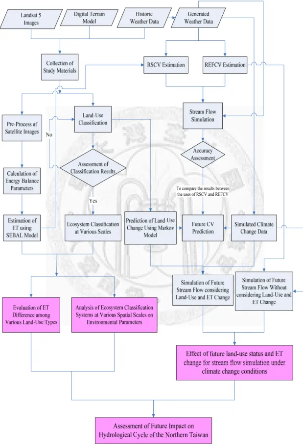
Figure 8. Flowchart of the study process………...….…...37
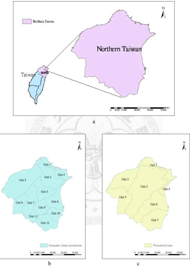
Figure 9. Spatial scales and two ecosystem classification systems………...42
Figure 10. The predicted time stages for future land-use conversions and CV values………...51
Figure 11. Spatial distribution of the selected blocks and test areas…………..…...55
Figure 12. Land-use maps generated by the hybrid classification……….…...59
Figure 13. Estimated energy balance parameters and ET maps of July 20, 1995...61
Figure 14. Estimated energy balance parameters and ET maps of November 25, 1995………62
Figure 15. Thiessen polygons and their influence coefficients………...66
Figure 16. Land-use maps of the Dan-Shuei watershed from 1995…...…………...71
Figure 17. ET maps of the Dan-Shuei watershed from 1995…...………...72
Figure 18. The observed and simulated hydrographs…...…………..………...74 Figure 19. Comparison of the predicted stream flows between the traditional
approach and proposed approach based on CGCM1 climate change model…...……….………..…………...81 F i g u r e 2 0 . C o mp a r i s o n o f h y d r o g r a p h s b e t w e e n c u r r e n t a n d f u t u r e
conditions…...………..…………...84
1. INTRODUCTION
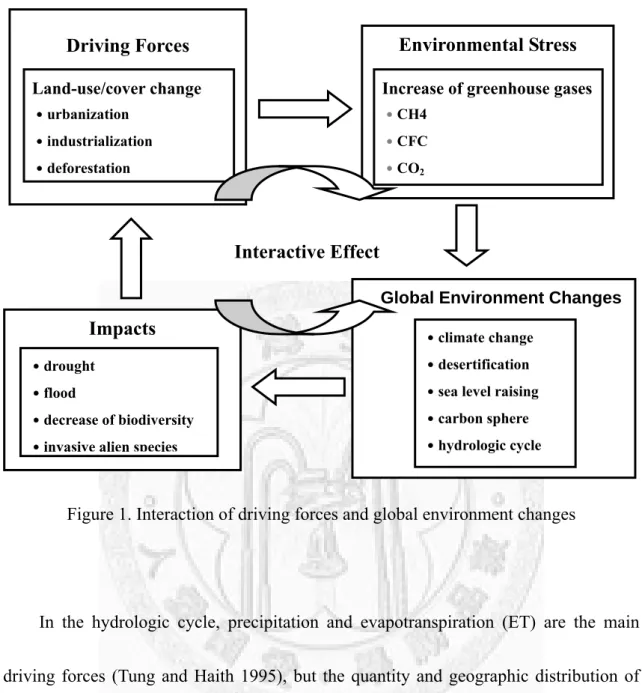
It is widely believed that an increased emission of greenhouse gases into the earth’s atmosphere has likely been occurring since the industrial revolution (Arnell and Reynard 1996). From 1750 to 2000 the concentration of carbon dioxide (CO2) and methane (CH4) increased 31 ± 4% and 151 ± 25%, respectively. Such a rapid increase not only enhances the green house effect, but also promotes the occurrence of global warming (Manning and Nobre 2001). Because of the importance of the issues, the United Nations Framework Convention on Climate Change (UNFCCC) was adopted in May 1992 and opened for signatures a month later at the United Nations Conference on Environment and Development (UNCED) in Rio de Janeiro, Brazil. The UNFCCC provides the basis for global action to protect the climate system for present and future generations. Considerable attention has been given to investigate the interactions among climate change, human activities, and nature ecosystems around the world (Figure 1).
Figure 1. Interaction of driving forces and global environment changes
In the hydrologic cycle, precipitation and evapotranspiration (ET) are the main driving forces (Tung and Haith 1995), but the quantity and geographic distribution of these two factors has changed due to the increase of the average temperature of the earth.
This phenomenon also affects other hydrological components such as infiltration, and stream flow, which in turn disturbs the available water resources for humans. If the current trend does not change, the impact of global warming on future climatic condition and hydrologic processes will become a major concern (Wu and Haith 1993).
Estimates of global warming are usually based on the application of General Circulation Driving Forces
Land-use/cover change
․urbanization
․industrialization
․deforestation
Environmental Stress
Increase of greenhouse gases
․CH4
․CFC
․CO2
Global Environment Changes Impacts
․drought
․flood
․decrease of biodiversity
․invasive alien species
Interactive Effect
․climate change
․desertification
․sea level raising
․carbon sphere
․hydrologic cycle
Models (GCMs), which attempt to predict the impact of increased atmospheric CO2
concentrations on climatic variables. In order to assess the sensitivity of hydrological regimes to the climatic changes associated with global warming, previous studies have often relied on the GCMs coupled with a stream flow model, and have used these models to predict the impact of climate change on hydrologic characteristics in different areas (Yu et al. 2002). To apply these models to global environment change, the acquisition of large-scale environmental information (e.g., daily ET amount) and land-use status are necessary. ET is traditionally calculated from records of weather stations or estimated by hydrological balance functions (Chiou, 2005). These methods are limited in their ability to provide point values of ET for specific locations and fail to provide ET on a regional scale. Regarding the acquisition of land-use data, traditional ground survey methods consume much effort, money, and time. The acquisitions of multi-temporal land-use information are also problematic.
Today, remote sensing technologies have become readily available because satellite images can easily and effectively provide large scale and multi-temporal surface information for many purposes, including forest hydrology studies. The application of these newer technologies provides a more appropriate means for determining the spatial and temporal structure of ET and land-use information. If the hydrological parameters and land-use information derived from remote sensing techniques could be integrated
with an impact analysis of climate change on hydrology, it will improve the predictability of climate change effects on water resources. The combination of remote sensing, GCMs models, and stream flow models will become an important issue for hydrology study.
2. MOTIVE AND OBJECTIVE
2.1. Motive
In recent years, physically based and semi-distributed models have been frequently used to address the influence of land-use change and climate change on hydrology (Weiler et al., 2005). The Generalized Watershed Loading Functions (GWLF; Haith and Shoemaker, 1987; Haith et al., 1992; Wu and Haith, 1993) model is one of the stream flow models that incorporates the physical mechanisms and water balance relationship within a watershed. The most important advantage of using the GWLF model is that parameters can be adjusted according to the land-use types, soil characteristics and climate conditions of a watershed. For this reason, the GWLF model has been widely applied to estimate human, natural, and climate effects on hydrologic systems (Tung and Haith, 1995; Fan, 1998; Cheng et al., 2007; Markel, 2006).
In previous studies, the amount of ET in a watershed was calculated using evapotranspiration cover coefficient (CV) during the GWLF simulated procedures. The CV for each land-use type is defined as a ratio of actual ET to potential evapotranspiration (PET). However, the estimation of actual ET and CV of a large spatial scale is problematic. For example, CV can be determined from the published seasonal values based on crop types such as those given in the user’s manual of the
GWLF model (Haith et al., 1992), this approach often requires estimates of crop development (e.g., planting dates, time to maturity, etc.) which may not be available.
Moreover, a single set of consistent values is seldom available for all of a watershed’s land-use, and settling for a cursory CV value could greatly reduce the accuracy of stream flow simulations (Haith et al., 1992, Davis and Sorensen, 1969).
The increasing availability of remote sensing technology now produces satellite images that can easily and effectively provide large scale spatial and temporal surface information. For hydrology studies, Actual ET can be computed without quantifying other complex hydrological processes through remote sensing techniques (Morse et al., 2000). Thus, much previous research adopted remotely sensed data to calculate the energy balance parameters such as surface temperature, net radiance, sensible heat flux, soil heat flux, and then estimated the actual ET according to these parameters (Chen et al., 2006; Laymon et al., 1998; Mauser and Scha¨dlich, 1998; Menenti and Choudhury, 1993; Morse et al., 2000). Most of these earlier studies focused on the comparison of ET among various spatial scale and temporal stages. However, few researches have calculated CV parameters using remote-sensing-based ET for the purpose of stream flow simulation. Investigations regarding the effects of land-use types and spatial scales on ET are also seldom attempted.
In addition to the climatic factors, land-use change will influence the amount of ET,
and thereby affect the balance of the hydrologic cycle (Cheng et al., 2007). In the GWLF model, parameters such as curve number (CN) and CV are related to the land-use status of a watershed. Most previous studies assumed that catchment land-use remains consistent over long periods of time (Arnell and Reynard 1996). This assumption may reduce the accuracy of prediction. Many existing spatial simulation models have been applied in various fields (Muller and Middleton 1994; Turner 1993).
A Markov model is the most widely used approach. In the Markov model, area change is summarized by a series of transition probabilities from one state to another over a specified period of time. These probabilities can be subsequently used to predict the land-use properties at specific future time points (Burham 1973). Many researchers have applied the Markov model to monitor the land-use and landscape change (Cheng et al.
2005; Lindsay and Dunn 1979; Muller and Middleton 1994; Turner 1993), but few integrate Markov predictions into hydrological assessments under changing climate conditions.
During watershed ecosystem monitoring, we observed that ecosystems are nested and reside within each other. The boundaries of ecosystems are open to transfer energy and materials to or from other ecosystems, and this linkage among systems, energy exchange to occur at various spatial scales. A disturbance to a large system may also affect smaller component systems existing within it. Consequently, the relationship
between an ecosystem at one scale and ecosystems at smaller or larger scales must be examined to predict the effects of human disturbances (Bailey, 1996, Cheng et al., 2005).
Previous research has focused on the effects of global and regional scales on environmental parameters (Rao, 1990; Tokumaru and Kogan, 1993; Yu et al., 2002;
Chen et al., 2006), but studies evaluate the issues of ecosystems at various scales and their effects on environmental parameters. A further investigation of the multi-scale relationship of environmental characteristics under various ecosystem classification systems is needed.
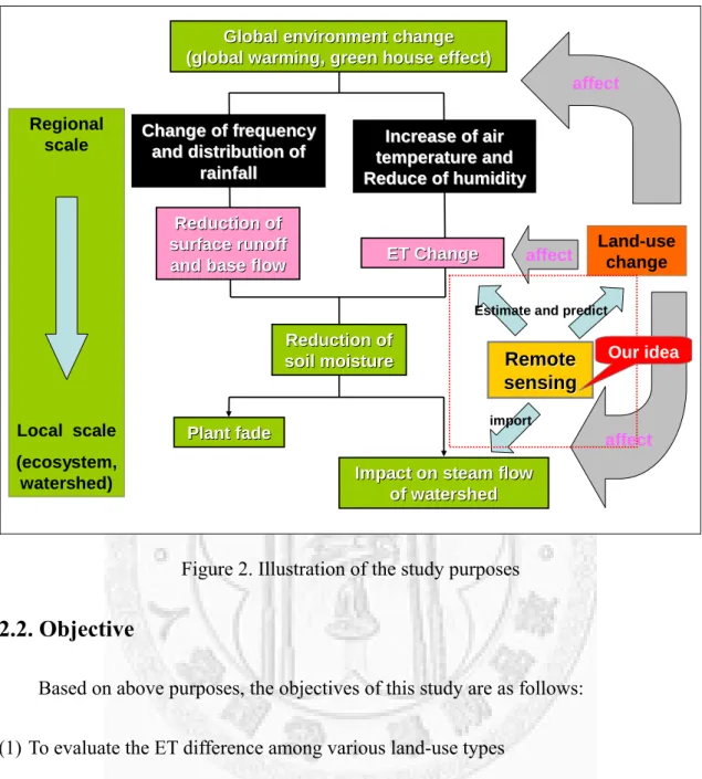
The northern part of Taiwan is a region which includes several political (ex. the capital city of Taiwan: Taipei city), scientific (ex. Hsin-chu science park), and agricultural centers (Lan-Yang flat land). These scientific or agricultural centers play important roles on technology development and crop supplies of Taiwan. An overall hydrological analysis is important in this area. Moreover, to realize how the hydrologic system would be changed in the future is also necessary for the water resource management. Figure 2 is an illustration of the study purposes.
Reduction Reductionof of surface runoff surface runoff and base flow and base flow Change of frequency Change of frequency and distribution of and distribution of
rainfall rainfall
Increase of air Increase of air temperature and temperature and Reduce of humidity Reduce of humidity
affect affect
Remote Remote sensing sensing
Land-use change affect affect
affect affect Regional
scale
Local scale (ecosystem,
watershed) Impact on steam flow Impact on steam flow of watershed of watershed Plant fade
Plant fade
Reduction of Reduction of soil moisture soil moisture
ET Change ET Change Global environment change Global environment change (global warming, green house effect) (global warming, green house effect)
Estimate and predict
import
Our idea
Figure 2. Illustration of the study purposes 2.2. Objective
Based on above purposes, the objectives of this study are as follows:
(1) To evaluate the ET difference among various land-use types
Land-use maps generated by a hybrid classification approach (Hoffer and Fleming, 1978, Lo and Choi, 2004) and daily actual ET obtained from Surface Energy Balance Algorithm for Land (SEBAL; Bastiaanssen et al. 1998a) are integrated to investigate the effects of land-use types on ET.
(2) To analyze the effect of ecosystem classification systems at various spatial scales on environmental parameters
Two spatial scales (regional scale and local) and ecosystem classification systems (geographic climate method and watershed division method) were adopted to assess their effect on environmental parameters.
(3) To investigate the effect of future land-use status and ET change on stream flow simulation under climate change conditions
Compared with the traditional stream flow simulation, which calculates a CV using the published reference values and without evaluating land-use change, our present efforts presents an approach to estimate CV by Markov model and SEBAL model, which includes future land-use status and ET change. Our study was motivated by the following three questions. Is the accuracy of stream flow simulation improved by using the CV estimated from remote sensing? Is the integration of SEBAL model and Markov model a feasible scheme to predict the future land-use and ET parameters for stream flow simulations? Does the consideration of land-use change and ET change affect the results of hydrologic assessment under climate change conditions in north Taiwan?
(4) To assess the future impact on hydrological cycle of north Taiwan
Flow series from 1995 to 2002 were adopted to represent the current hydrological condition, and then compared with the future flows to investigate how land-use change, ET change, and climate change affected river flows and the hydrologic cycle of north Taiwan.
3. LITERATURE REVIEW
3.1. Land-Use Classification using Remote Sensing
Classification of land-use and land cover using satellite images is considered an essential task in modeling the earth as a system. Traditionally, supervised and unsupervised classifications are two common image classification approaches, each with advantages and disadvantages (Lillesand and Kiefer, 2004; Lang et al., 2008). The supervised approach involves a training stage, which allows the input of analyst’s experience into image classifications. However, this approach has been regarded as overly subjective and difficult to correctly implement, because user-defined training data may not be normally distributed. The unsupervised approach can automatically generate almost unlimited number of spectral classes, which are solid spectral foundations for generating information classes, but it requires the analyst manually label the resultant spectral classes into information classes (Lang et al., 2008).
To improve the accuracy of image classification, an integrated algorithm called a hybrid classification approach that takes advantage of both classification approaches has been developed (Hoffer and Fleming, 1978, Lo and Choi, 2004). In this hybrid approach, cluster analysis was first used to acquire the spectral signatures objectively, and then the signature file was imported into the supervised classification to generate the land-use
map. Hybrid classification has been widely applied in ecosystem monitoring studies, and the results from previous studies demonstrated that the integrated algorithm could provide an accurate and consistent classification of land use mapping. For example, Lo and Choi (2004) adopted the hybrid classification method to map the land use/cover of the Atlanta metropolitan area using Landsat 7 Enhanced Thematic Mapper Plus (ETMz) data; Lang et al. (2008) applied the hybrid approach to generate a land-use map of Indiana, USA. Lillesand and Kiefer (2004) indicated that the hybrid approach indeed increased the repeatability and accuracy of land-use classification.
3.2. Estimation of Environmental Parameters and ET based on the SEBAL Methodology
SEBAL is an image processing model that calculates the actual ET and other energy exchanges at the earth’s surface using digital image data collected by Landsat or other remote sensing satellites measuring visible, near infrared, and thermal infrared radiation (Bastiaanssen et al., 1998a). The major concept of this model is that ET flux is calculated as a residual of the surface energy budget equation and is expressed as the energy consumed by the evaporation process:
H G Rn
LE 0 (1)
where, LE is the latent heat flux (W/m2); Rn is the net radiation flux at the surface (W/m2); G0 is the soil heat flux (W/m2); H is the sensible heat flux to the air (W/m2). LE is converted into ET, expressed as a depth of water per time, by dividing by the latent heat of vaporization.
Sensible Heat Flux
SEBAL Model Digital Terrain
Model data
Satellite Image (Landsat)
Normalize Difference Vegetation Index
Net Radiation
Soil Heat Flux
Wind Speed Information Evapotranspiration
Radiation Balance for
the Land Surface
Figure 3. General computational process for determining ET using SEBAL (Morse et al., 2000)
Figure 3 is the schematic of the general computational process for determining ET using SEBAL. During the model processes, actual ET is computed as a component using 15 energy balance parameters, including the cosine of solar incidence angle (cosθ;
unitless), twenty-four hour extraterrestrial radiation (Ra24; W/m2), surface albedo at the top of atmosphere (αtoa; unitless), surface albedo (α0; unitless), normalized difference vegetation index (NDVI; unitless), emissivity (ε0; unitless), surface temperature (T0; K), transmittance (τsw; unitless), air density (pair; kg/m3), aerodynamic resistance to heat transport (rah; s/m), estimating friction velocity (u*; m/s), surface roughness for momentum transport, (zom; m), net radiation (Rn; W/m2), soil heat flux (Go; W/m2), sensible heat flux (H; W/m2) (Morse et al., 2000). In SEBAL procedures, Rn was estimated based on the following relationship (Bastiaanssen et al., 1998; Oberg and Melesse, 2004):
) 1 ( )
1
( 0
s L L L
n R R R R
R ( 2 )
where, R
S↓is the incoming direct and diffuse shortwave solar radiation that reaches the surface (W/m2); α is the surface albedo, the ratio of reflected radiation to the incident shortwave radiation; R
L↓is the incoming longwave thermal radiation flux from the atmosphere (W/m2); R
L↑is the outgoing longwave thermal radiation flux emitted from the surface to the atmosphere (W/m2); ε
o is the surface emissivity, the ratio of the radiant emittance from a gray body to the emittance of a blackbody.
Soil heat flux (G0) is the rate of heat storage to the ground from conduction. In the
SEBAL model, an empirical relationship for G0 was given as:
Rn
NDVI
G0 0.30(10.98 4) (3)
where, NDVI is the normalized difference vegetation index.
Sensible heat flux (H) is the rate of heat loss to the air by convection and conduction due to a temperature difference. The calculated equation was as bellow:
ah p
r dT H C
(4)
where, ρ is the density of air (kg/m3); c
p is the specific heat of air (1004 J/kg/K); dT is the difference in temperature between the surface and the air (K); and r
ah is the aerodynamic resistance (s/m). To calculate dT, the inverse of equation (5) was considered:
p ah
C r dT H
(5)
Therefore, during the SEBAL process, the user calculated dT at two extreme
“anchor pixels” by assuming values for H at the reference pixels. The reference pixels were carefully chosen so that at these pixels one can assume that H approximate zero at a very wet pixel (i.e., all available energy (Rn - G0) is converted to ET), and that LE almost equals zero at a very dry pixel, so that H = Rn - G0. These assumptions from the selected pixels provided endpoints for values and locations for H so that a relationship for dT can be established.
Once the values of H and G0 were calculated, the latent heat flux (LE) can be calculated from equation (1). This LE represented the instantaneous evapotranspiration at the time of the Landsat overpass. Following the computation of the evaporative fraction at each pixel of the image, one can estimate the 24-hour evapotranspiration for the day of the image by assuming that the value for the evaporative fraction ( ) is constant over the full 24-hour period (Bastiaanssen et al. 1998). The evaporative fraction is calculated for the instantaneous values in the image as:
0 0
G R
H G R
n n
(6)
where, the values for Rn, G0, and H are instantaneous values taken from processed images. The 24 hour actual evaporation is calculated by the following equation:
) (
86400 24 24
24
G
ET Rn
( 7 )
where, ET24 is daily actual evapotranspiration (cm/day); Rn24 is daily net radiation; G24
is daily soil heat flux; 86,400 is the number of seconds in a twenty-four hour period; and λ is the latent heat of vaporization (J/kg). The latent heat of vaporization allows
expression of ET24 in cm/day.
Many previous studies applied remotely sensed data to calculate the energy balance parameters, and then estimated the actual ET according to these parameters. For example, Chen et al. (2006) applied the SEBAL model and four seasons of moderate resolution imaging spectroradiometer (MODIS) satellite images to estimate ET for the entire island of Taiwan; Laymon et al. (1998) used Landsat thematic mapper (TM) images and experience functions to estimate energy fluxes and latent heat flux, and further to calculate the ET in a semidesert area of West America; Mauser and Scha¨dlich (1998) modeled the spatial distribution of ET on a different scale using remote sensing data; Menenti and Choudhury (1993) applied Landsat MSS data to develop the surface energy balance index (SEBI) model, and then to estimate the ET of the Libyan desert in West Africa by using surface albedo and aerodynamic roughness; Morse et al. (2000) applied the SEBAL model and satellite images to calculate the ET, and the results showed that the R2 value between ET acquired from remote sensing and observed data
was 0.98.
Physical parameters obtained from the SEBAL model also have special meanings on the description of temperature, vegetated, hydrological and energy characteristics of an ecosystem. For example, Ra24 is the daily incoming solar radiation unadjusted for atmospheric transmittance; αtoa and α0 indicate the ratio of reflected to incident solar radiation at the atmosphere and ground surface; ε0 and T0 are temperature indices which denote the thermal energy radiated by the surface and surface temperature conditions of the area; NDVI is a sensitive indicator of the amount and condition of green vegetation;
zom is defined as the height above the “zero-plane displacement” that the zero-origin for the wind profile just begins within the surface or vegetation cover; Rn is the net radiant energy that the land surface actually receives and loses from or to the atmosphere. The allotment of Rn represents the energy transmission process within the ecosystem. Rn is divided into three components; ET24 is the twenty-four hour actual evapotranspiration. It also indicates the energy that used to support the photosynthesis and evaporate soil water; H is the energy used to heat the air; Go is the rest of the net energy which is stored in the ground or water body. The above environmental parameters were computed by the SEBAL model based on an energy balance algorithm. However, the acquisition of surface reflectance would vary with different terrains and meteorological conditions. For instance, the instantaneous and 24-hour solar radiations on a south slope
are much higher than on a north slope in the Northern Hemisphere. Atmospheric humidity and soil moisture are two important factors for ground reflectance, and they might influence the calculation of environmental parameters (Cheng et al., 2008).
3.3. Climate Change Scenarios
Climate change is a very complex issue. Policymakers need an objective source of information about the causes of climate change, its potential environmental and socio-economic consequences, and the adaptation and mitigation options to respond to it. This is why World Meteorological Organization (WMO) and UNEP established the Intergovernmental Panel on Climate Change (IPCC) in 1988.
The IPCC is a scientific body. The information it provides with its reports is based on scientific evidence and reflects existing viewpoints within the scientific community.
The comprehensiveness of the scientific content is achieved through contributions from experts in all regions of the world and all relevant disciplines including, where appropriately documented, industry literature and traditional practices, and a two stage review process by experts and governments.
The IPCC currently has three Working Groups and the Task Force on National Greenhouse Gas Inventories. The Working Groups and the Task Force have clearly defined mandates as agreed by the Panel and their activities are guided by two Co-chairs
each. They are assisted by a Technical Support Unit and the Working Group or Task Force Bureau. Working Group (WG )Ⅰ Ⅰ deals with "The Physical Science Basis of Climate Change", Working Group Ⅱ (WG ) with "Climate Change Impact, Ⅱ Adaptation and Vulnerability" and Working Group (WG ) with "Mitigation of Ⅲ Ⅲ Climate Change". The main objective of the Task Force is to develop and refine a methodology for the calculation and reporting of national green house gas emissions and removals. In addition to the Working Groups and Task Force, further Task Groups and Steering Groups may be established for a limited or longer duration to consider a specific topic or question (IPCC, 2004).
At regular intervals, the IPCC provides assessment reports of the state of knowledge on climate change, which become standard works of reference, widely used by policymakers, experts, and students. The findings of the first IPCC Assessment Report of 1990 played a decisive role in leading to the United Nations Framework Convention on Climate Change (UNFCCC), which was opened for signature at the Rio de Janeiro Summit in 1992 and enacted in 1994. It provides the overall policy framework for addressing the climate change issue. The IPCC Second Assessment Report of 1995 provided key input for the negotiations of the Kyoto Protocol in 1997, and the Third Assessment Report of 2001, as well as Special and Methodology Reports, provided further information relevant for the development of the UNFCCC and the
Kyoto Protocol. The IPCC continues to be a major source of information for the negotiations under the UNFCCC. The latest one is "Climate Change 2007", the Fourth IPCC Assessment Report (IPCC, 2007).
In 2000 the IPCC published a new set of emission scenarios, which address changes in the understanding of driving forces and emissions and methodologies since the completion of the IPCC IS92 scenarios. The Special Report on Emissions Scenarios (SRES) are based on an extensive assessment of driving forces and emissions in the literature, alternative modeling approaches and an “open process” that solicited participation and feedback from scientist’s around the world. An important part of this report is the consideration of the contributions to future emissions, from demographic to technological and economic developments, but, as requested in the terms of reference, none of the scenarios included future policies that explicitly address climate change.
Four different storylines were developed to describe the relationship between emission driving forces, and their evolutions, and add context to the scenario quantification (IPCC, 2000).
3.4. Application of the GWLF Model on Hydrologic Monitoring
The GWLF model is a physical hydrological model, which simulates the water balance within an upstream watershed. In the GWLF model, the stream flow consists of
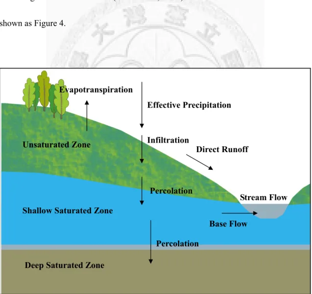
runoff and discharge from groundwater. The latter is obtained from a lumped parameter watershed water balance. Daily water balance is calculated for unsaturated and shallow saturated zones. Infiltration to the unsaturated and shallow saturated zones equals the excess, if any, of rainfall and snowmelt less runoff and ET. Percolation occurs when unsaturated zone water exceed field capacity. The shallow saturated zone is modeled as a linear groundwater reservoir (Haith et al., 1992). The model structure of GWLF is shown as Figure 4.
Figure 4. Water balance function of the GWLF model (modified from Haith et al., 1992)
Deep Saturated Zone Shallow Saturated Zone Unsaturated Zone
Evapotranspiration
Effective Precipitation
Infiltration
Percolation
Direct Runoff
Base Flow
Stream Flow Percolation
t t
t G Q
SF ( 8 )
where, SFt is the stream flows of a watershed (cm); Gt is the groundwater discharge (cm); Qt is the surface runoff (cm).
Groundwater discharge is estimated by assuming shallow saturated zone as a linear reservoir using the follow equation:
t
t S
G r ( 9 )
where, r is the recession coefficient; St is the storage of shallow saturated zone (cm).
To estimate surface runoff, the GWLF model used the curve number method to calculate runoff volumes with the considerations of land-use status and antecedent soil moisture. The equations are as follows:
) 8 . 0 (
) 2 . 0
( 2
t t
t t
t R W
W Q R
(10)
4 . 2540 25
t
t CN
W CN 100 (11)
where, Qt is the surface runoff (cm); Rt is the daily precipitation (cm); CN is the curve number; Wt is the maximum soil runoff load (cm).
Curve number is selected as functions of land use types, soil texture and antecedent moisture. Curve number for antecedent moisture conditions 1 (driest), 2 (average) and 3 (wettest) are CN1, CN2, and CN3, respectively. CN2 can be determined by referring to the GWLF manual, and CN1 and CN3 can be calculated from CN2. The functions of CN1 and CN3 are as follows (Haith et al., 1992):
2 0059 . 0 4036 . 0 3 2
2 01334 . 0 334 . 2 1 2
CN CN CN
CN CN CN
(12)
Moisture leaves the ground surface of a watershed as ET, that is, transpiration by plants and evaporation from moist soil and the stream surface (Weisman, 1977).
Estimation of ET for watershed studies is problematic (Haith et al. 1992). In the GWLF model, ET is estimated as a function of the atmospheric and surface characteristics of a watershed, as equation (8).
t
t CV PET
ET (13)
where, ETt is evapotranspiration (cm); CV is cover coefficient; PETt is potential evapotranspiration (cm) as given by Hamon (1961):
273 021 .
0 2 0
t
t t t
T e
PET H (14)
where Ht is the number of daylight hours per day during the month containing day t; e0t
is the saturated water vapor pressure in millibars on day t, and Tt is the temperature on day t ( ). Saturated water vapor pressure can be approximated as in Bosen (1960):℃
00136 . 0 8 . 4 8
. 1 000019 .
0 8 . 0 ) 8072 . 0 00738
. 0 [(
8639 .
0t 33 Tt Tt
e (15)
In urban areas, ground cover is a mixture of trees, grass, water, and concrete constructions. It follows that CV for an area are weighted averages of the perennial crop, hardwood and softwood forest, water, and construction factors, as equation (16) and (17).
t i
i PET
cv ET (16)
m
i
i i
e cv w
CV
1
(17)
where, cvi is CV of class i; ETi is ET of class i (mm/day); CVe is the CV for the entire area; wi is percentage of class i; PETt is potential evapotranspiration (cm).
Stream flows calculated by the GWLF model are based on a consideration of water balance within a watershed. Compared with other models, the GWLF model uses fewer parameters but processes a high degree of predictive accuracy. Consequently, many studies (Haith et al., 1992; Tung et al., 1999; Yu et al., 2002; Markel et al., 2006) applied the GWLF model to assess the watershed hydrology and stream flow volume, and also to validate the flow prediction of the GWLF model. For example, Haith et al.
(1992) tested the GWLF model by comparing model predictions with measured stream flow from the West Branch Delaware River Basin (area = 850 km2) during a three-year period. The result showed that the derived coefficient of determination (R2) is 0.88, indicating that the model explains at least 88% of the observed monthly variation in stream flow. Although better results could perhaps be obtained by more detailed hydrologic models, such models have substantially greater data and computational requirements and must be calibrated from sampling data.
Many previous studies often rely on the GCMs coupled with the GWLF model to assess the sensitivity of hydrological regimes to the climatic changes associated with global warming (Yu et al. 2002). For example, Tung and Haith (1995) used the GWLF model and two kinds of GCMs scenarios to asses the impacts of global warming on stream flows for four large watersheds in New York State. Fan (1998) developed a procedure to evaluate the impacts of climate change on ground water recharge in Taiwan using the GWLF model and four climate change scenarios. Cheng et al. (2007) integrated the Markov model and the SRES scenario to investigate the influence of future land-use changes and climate changes on the stream flow simulations using the GWLF model, and also to assess the impacts on the Jiao-Long watershed of central Taiwan.
3.5. Prediction of Land-Use Change using Markov Model
The Markov model is a stochastic model. During its process, land-use change of an area is summarized by a series of transition probabilities from one state to another over a specified period (Hillier and Lieberman, 1995). These probabilities can be subsequently used to project the landscape properties at alternate future time points (Burham, 1973).
The Markov model assumes that the land-use changes of the study area could be
depicted as a Markov process. A transition matrix, in which the element Tij represents the amount of land-use change from type i to type j during two periods, are derived from the land-use maps (Cheng, et al., 2006). The transition probability Pij, which represents the factions of land-use changes on each land-use type, is estimated by:
m
j ij
ij Tij T
P
1
; i = 1, 2, ... m, (18)
where, m is the number of land-use types.
To determine whether it is appropriate to apply the Markov model to the observed land-use changes, Goodman’s Chi-squared statistic (Goodman 1968) was used to test the null hypothesis that the land-use conditions in 1995 and 2002 were independent of each other. If the calculated α2 is larger than the reference value, we reject the hypothesis that land-use change during the period is a random procedure. In other word, the transition process is a Markov chain procedure. We can apply the Markov model to predict the possible land-use change of the area.
2 21 1
2 ln( ) ; ( 1)
m df A
P
m T
i m
j ij ij j
(19)
where, the definitions of Tij and Pij are same as in equation (18), Aj is the fraction of land-use in each of the land-use types in 1995; df is the degree of freedom.
Assuming that the transition probabilities will remain constant in the future, the Markov model is then used to project the land-use at the next stage:
1
2 t
t P n
n (20)
where, P is the transition probability matrix, nt1 and nt2 are column vectors denoting the fractions of land-use types at t1 and t2.
The Markov model is a widely used approach to evaluate the change of land-use types, landscape distribution, and ecosystem environment (Wu, 2004). For example, Turner (1993) used the Markov transition probability to monitor the landscape changes in nine rural counties in Georgia, USA; Avaiksoo (1995) simulated the vegetation dynamics and land use in a mire landscape using a Markov model; Hsu and Cheng (2000) assessed the landscape change in Liukuei ecosystem area using a Markov model.
Lindsay and Dunn (1979) applied a transition matrix approach to project the land use
simulate the land-use change dynamics in the Niagara Region, Ontario, Canada.
This present study will contribute to these past efforts by proposing a hybrid of SEBAL, GCMs, and GWLF models in order to simulate more accurate hydrological change based on climate change conditions.
4. STUDY AREA and MATERIALS
4.1. Study Area
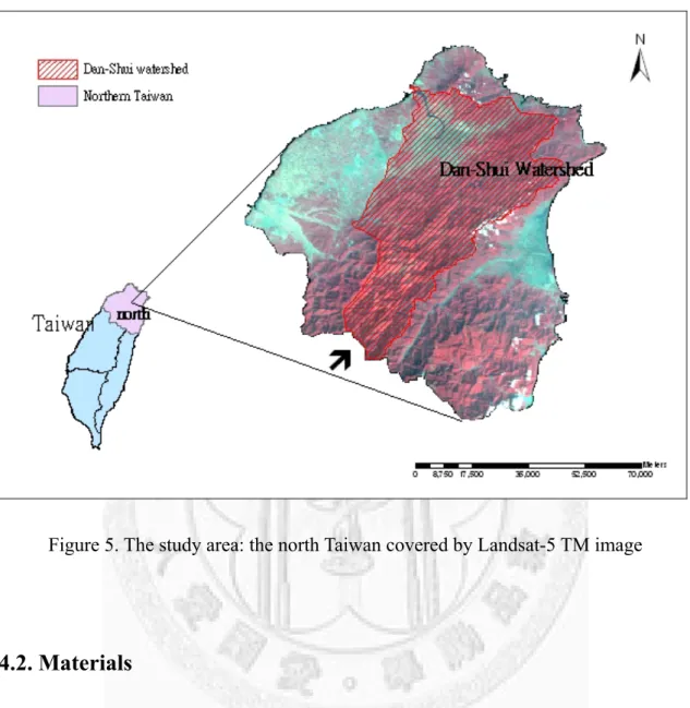
The study area selected for the empirical analysis was the north of Taiwan. There are four main streams (Dan-Shui river, Kee-Lung river, Xin-Dian river, and Da-Han creek) in this area, which divide the region into seven watersheds. The area covers 734589.7 ha and involves five counties (Kee-Lung, I-Lan, Taipei, Tao-Yuan, and Hsin-Chu). Many land-use and cover types exist in this area, such as industrial and business center (e.g., Taipei city), scientific parks (e.g., Hsin-Chu science parks), mountainous forest area (e.g., I-Lan county), farmland (e.g., Lan-Yang plain) and ponds (e.g., Tao-Yuan county). Several industrial or scientific centers in this area demand water resource. Therefore, it is important to predict how the hydrologic system could change in the future. Figure 5 is the location of study area.
Figure 5. The study area: the north Taiwan covered by Landsat-5 TM image
4.2. Materials
Five kinds of data were consulted for this study, Landsat-5 TM images of 1995 and 2002, digital terrain model (DTM), national land-use inventory data in 1995, and daily observational records of weather and stream flow. First, three Landsat-5 TM images from different dates (July 20 and November 25, 1995; January 4, 2002) were adopted.
Landsat-5 TM images contain seven spectral bands ranging from the visible blue to the middle infrared (mid-IR). Bands 1 to 3 are the blue, green, and red bands; band 4 is the
near IR; band 5 and band 7 are the mid-IR. Each of above six bands has a 30 m ground resolution. Band 6 is the thermal IR with 120 m resolution. The extent of the study area was clipped from the raw images and used to generate land-use maps. Second, DTM with 40 m resolution was provided by the aerial survey office, Forestry Bureau. The DTM data was used to derive the slope, aspect, and elevation information for modification of the SEBAL model in a mountainous area. National land-use inventory data generated in 1995 by the Department of Land Administration, the Ministry of the Interior is regarded as the paragon for evaluating image classification. The period from 1995 to 2002 was selected as the baseline, representing “current climatic conditions”.
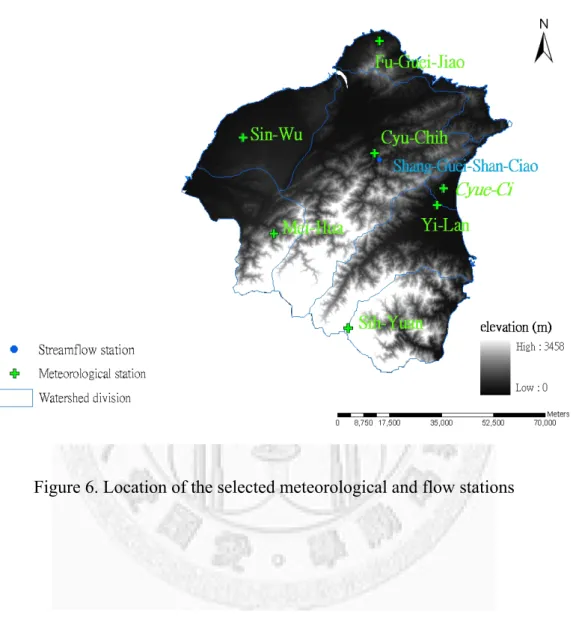
Daily temperature and precipitation data were collected from seven meteorological stations. These are: Fu-Guei-Jiao, Cyu-Chih, Sin-Wu, Cyue-Ci, Mei-Hua, Yi-Lan and Sih-Yuan weather stations. The Dan-Shui watershed, which occupies the largest drainage area in north Taiwan, was assigned to be the sample for model validation.
Climatic records at the Cyu-Chih meteorological station and stream flow observations at Shang-Guei-Shan-Ciao flow station were collected from 1995 to 2002. Although the distance between two gauged stations is less than 1 km, both stations have similar elevation (Cyu-Chih station: 90.0m; Shang-Guei-Shan-Ciao station: 70.9m). Thus the meteorological stream flow data collected from these two stations is comparable for hydrological analysis. Figure 6 shows the location of the selected meteorological and
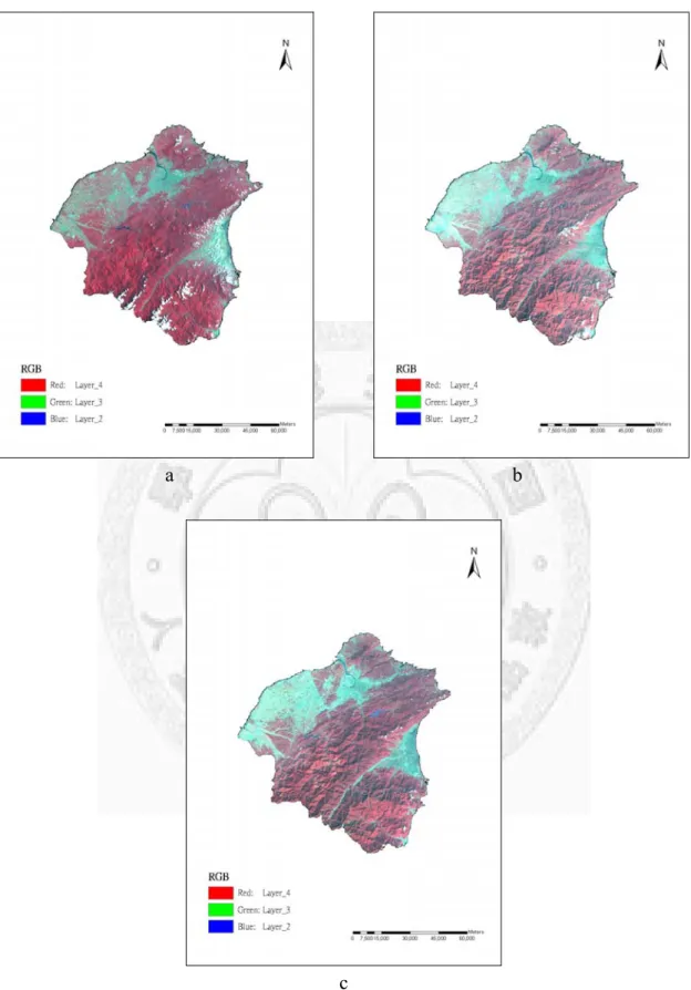
flow stations. Figure 7 shows the Landsat-5 TM images used in this study.
Figure 6. Location of the selected meteorological and flow stations
a b
c
Figure 7. Landsat-5 TM images of the north Taiwan in three dates
(a: July 20, 1995; b: November 25, 1995; c: January 4, 2002)