應用分數檢定統計量於選擇性基因型試驗之數量性狀基因座定位研究

(1)

國立臺灣大學生物資源暨農學院農藝所生物統計組碩士論文

Division of Biometry Graduate Institute of Agronomy College of Bioresources and Agriculture

National Taiwan University Master Thesis

應用分數檢定統計量於選擇性基因型試驗之數量性狀基因座定位研究

Score Test Statistics for QTL Mapping under Selective Genotyping

房佑嬙

Yu-Chuang Fang

指導教授：高振宏博士、廖振鐸博士

Advisor: Chen-Hung Kao, Ph.D. & Chen-Tuo Liao, Ph.D.

中華民國 102 年 7 月

July, 2013

(2)

口試委員審定書

(3)

謝誌

兩年的碩班生涯晃眼即逝，本篇論文如期完成最要感謝一路悉心提點、耐性指導的

高老師，並感謝在生活和學業上均給予諸多鼓勵的廖老師以及專程從花蓮北上指

導口試的靖老師。也謝謝研究室的學長姐們不嫌棄我的愚拙，不論大小事總是熱心幫忙解惑。最後感謝伴我成長的好夥伴---林昭京，謝謝你。

僅以此獻給育我劬勞的父母

(4)

中文摘要

生物上許多重要的經濟、生理、或與生化有關的性狀均為數量性狀。這些控制數量性狀的基因稱為數量性狀基因座 (Quantitative trait loci)，其定位與研究一直是

作物和動物在遺傳育種上的重要課題。利用分子遺傳標誌資料，數量性狀基因座定位 (QTL mapping)方法可幫助我們了解 QTL 在染色體上的位置及其作用大小。選

擇性基因型鑑定 (Selective genotyping)是一種只針對樣本族群之外表型極大與極

小的部分個體進行基因型鑑定的方法，它除了降低遺傳鑑定的成本外，一般認為也可以增進定位數量性狀基因座的效率。本篇文章中，利用 Lee et al. (2013) 針對選

擇性基因型鑑定所提出的兩種模式 (事後檢定模式與目前所行的模式)，分別推導

其分數檢定統計量(score test statistics)作為另一種定位 QTL 的統計量，並研究其在

選擇性基因型鑑定方法下的顯著性門檻值。結果發現，在單一QTL 存在的假設情

況下，兩種分數檢定統計量表現的一樣好。未來研究中，我們期待將單一QTL 假

設推廣至多個QTL 存在的情況，進行選擇性基因型鑑定之數量性狀基因座定位研

究。

關鍵字: 數量性狀基因座；數量性狀基因座定位；區間定位；分數檢定；選擇性基

因型鑑定

(5)

ABSTRACT

The detection of quantitative trait loci (QTL) that govern many biologically and

economically important traits is an important task in plant and animal breeding. Using

genetic marker data, QTL mapping technique has been known to be an efficient tool to

detect QTL location and estimate their effects. In QTL mapping, selective genotyping,

which genotypes only the individuals from high and low phenotypic values, is one of the

most common strategies that can reduce the cost of marker genotyping and at the same

time increase efficiency in QTL detection. In this thesis, with the posterior model of

selective genotyping proposed by Lee et al. (2013), we derived score test statistic for the

model and applied it to QTL detection. Moreover, we compare this score test statistics

with that of the currently used model, and the threshold values of the score test statistics

under selective genotyping are also investigated. As the result, we found out that the two

score test statistics for the posterior model and currently used model perform equally well

under single-QTL model. In the future, we intend to extend the single-QTL posterior

model to multiple-QTL model for QTL detection under selective genotyping.

KEYWORDS: QTL; QTL mapping; interval mapping; score test statistic; selective

genotyping

(6)



^{0 ,}^²



, a and d are the additive and dominance effects of Q, x_i^* and z^*_i defined as

(12)

*

1 if the genotype of Q is QQ, 0 if the genotype of Q is Qq, 1 if the genotype of Q is qq, xi  





and ^* 12 if the genotype of Q is Qq, 12 otherwise, zi  



in section 2.3 mentioned that Q is not observed but can be inferred from interval flanking

markers, the Q can be QQ



^x^*ⁱ ^^1,^zⁱ^*^{ }¹₂



^{, Qq}



^xⁱ^*^{ }^1,^z^*ⁱ ^¹₂



^{or qq}



^xⁱ^*^{ }^1,^zⁱ^*^{ }¹₂



for an individual i.

At a given position, for a sample of N individuals, the sum of the log likelihood function

of the model in Equation (1) is



₂

 

₂



³

 

²

1 1 2

, , , log 2 log exp

2 2

N i j

i j ij

N y

l a d p 

  

  

   

  

  

      

 

⁽²⁾

where p_ij is the conditional probability of QTL for ith individual, and

 

2 1

1 1

2 2 2 2

3 3 2 3

with probability , , 2

If Q is with probability , , 2

with probability , , 2

i i i

a d

QQ p N

Qq p N d

qq p N a d

 

 

   

   

  



   





which can be determined by the given position, and need not to be estimated here.

2.3 Statistical Model of QTL Mapping for Selective Genotyping

2.3.1 Statistical Model

Applying the statistical model to selective genotyped data analysis, we have to

separate the individuals into two parts: one of them is genotyped individuals

 

n , the other is ungenotyped individuals



N n



. Then the sum of the log likelihood function

(13)

becomes

     

 

3 2

2 2

1 1 2

3 2

1 1 2

, , , log 2 log exp

2 2

log exp

2

n i j

i j ij

N i j

i n j j

N y

l a d p

q y

   







 

  

   

  

  

      

   

  

  

    



 

 

 

(3)

where p_ij is the conditional probability of QTL for ith individual in selective genotyped

individual, which can be determined by the given position and need not to be estimated.

qj is the conditional probability of QTL for ungenotyped individuals, which have to be inferred from the posterior probability of ungenotyped flanking markers. According to

the model proposed by Lee et al. (2013), we derived posterior model to estimate q_j in

comparison with the prior model by using the score test statistic. Note that the log

likelihood for ungenotyped individuals have the same mixing proportions, q_j.

2.3.2 The Genotypic Structure of QTL in Ungenotyped Individuals

In the data analysis of selective genotyping, however, we only have the genotyped

data of extreme individuals. For those ungenotyped individuals, we have to speculate the

genotypic distribution of QTL according some rules.

Consider a QTL (Q), in the F2 population in which the frequency of genotypes QQ, Qq and qq are ¹₄, ¹₂and ¹₄, respectively. In general, Q is not observed but can

be inferred from the interval flanking markers according to the principle of conditional

(14)

probability as

   

 

| , P MQN P Q M N

 P MN . (4)

In F2 population, the two flanking markers have nine different genotypes, and for each

one of them, the genotype of the flanked Q can be QQ, Qq or qq. Thus, when considering

the flanking markers and the QTL (M, N and Q) together, there are 27 different

conditional probabilities. For example, the conditional probability for QTL given the

marker genotype ^MN_MN is P QQ| MN MN

 

 

 ^, P Qq| MN MN

 

 

 ^and P qq| MN MN

 

 

 ^{. For the} genotyped individuals, we used conditional probability which is proposed by Kao and

Zeng (1997) in Table 1 as the mixing proportion (p_ij) for the frequency of putative QTL

genotypes in the genotyped individuals. For the ungenotyped individuals, Xu and Vogl

(2000) applied currently used method ( (P QQ P Qq P qq ) : ( ) : ( ) 1: 2 :1) to represent the

mixing proportion (q_j ) for genotypic distribution of QTL based on ungenotyped

individuals. However, the frequencies of QTL genotype for ungenotyped individuals do

not follow the prior model under selective genotyping, for the reason that the extreme

individuals includes the same genotype practically which lead to the movement of the

frequencies of QTL for ungenotyped individuals and break the assumption of prior model

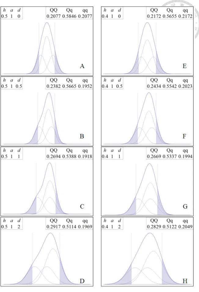
(Figure 1).

(15)

Figure 1: Normal mixture of phenotypic value. Based on different ℎ², 𝑎𝑎 𝑎𝑎𝑛𝑛𝑎𝑎 𝑎𝑎.

(16)

In this thesis we used posterior probability, which is proposed by Lee et al. (2013),

as the mixing proportion (q_j) trying to estimate the approximate probability of the QTL

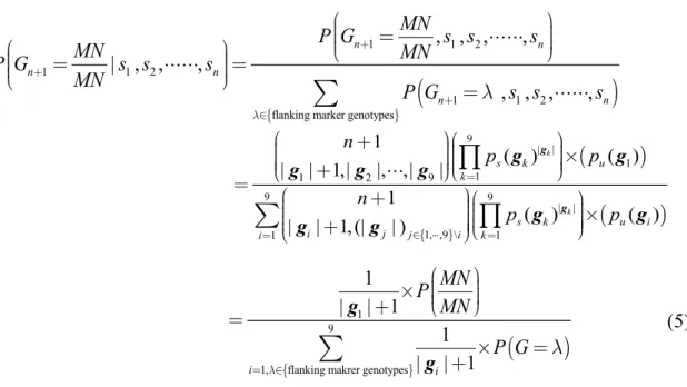
genotypes from ungenotyped individuals. First, we have to estimate the flanking marker

genotypes for ungenotyped individuals, the rule of posterior probability:

 

 

1 1 2

flanking marker genotypes

, , , ,

| , , ,

, , , ,

n n

P G MN s s s

MN MN

P G s s s

MN P G s s s







 

   

 

   

   

 

 



 

 

   

9 | |

1 1

1 2 9

9 9

| | 1, ,9 \ 1

1

1 1 2

1 ( ) ( )

| | 1,| |, ,|

| , |

1 ( ) ( )

|

, ,

| 1,(| | )

k

s k u

k

s k u i

i n

k i

n

j j i

P G MN s

n p

N n

M p p

s

p

s ^

 







   

  

  

    

 

     

 

   

 

 



 

g

g g

g g g

g g

 

 

9 1

1, flanking makrer genotypes

1 | 1 2

1

| | 1

| 1

, 1

|

, ,

i i

n MN n

P

M

G s s s

MN

P N MN

P G



 



 

  

   

 

 

  

 

 



 g

g

(5)

where the nine different flanking marker genotypes (λ) are the same as these listed in

Table 1. And in section 1 ,

n

is the total size of selective genotyped individual.

9 1

i|

i

n





^{| g}  ^,

^{| g}

ⁱ

^|

represent the number of each flanking marker genotypes in selective

genotyped individuals respectively. Second, the QTL conditional probabilities of

ungenotyped individuals ( 𝑞𝑞_𝑗𝑗) can be inferred from those posterior probabilities of

flanking markers by using Table 1.

(17)

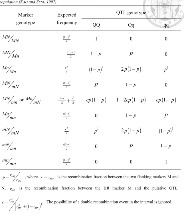
Table 1: Conditional probabilities of a putative QTL given the flanking marker genotypes for an F2

population (KAO and ZENG 1997)

Marker genotype

Expected frequency

QTL genotype

QQ Qq qq

MNMN ^ ^

1 2 4

r

 1 0 0

MNMn ^{ }¹2

r r 1 p p ₀

MnMn 4²

r



1 p



² 2 1p



p



p²

MNmN ^{ }¹2

r r p 1 p 0

MN or Mn

mn mN ^¹2^ 2²

r r

  cp



1p



1 2 1 cp



p



cp



1p



Mnmn ^{ }¹2

r r 0 ^{1 p}^ p

mNmN 4²

r p2 2 1p



p

 

1 p



²

mNmn ^{ }¹2

r r 0 p 1 p

mnmn ^ ^

1 2 4

r

 0 0 1

MQ MN

pr r , where rr_MN is the recombination fraction between the two flanking markers M and N, r_MQ is the recombination fraction between the left marker M and the putative QTL.

 

2

2 1 2

MN

MN MN

c r

r r

    

. The possibility of a double recombination event in the interval is ignored.

(18)

2.4 Score Test Statistics for Detecting QTL in Selective Genotyping

Under our proposed model (Equation (3)), score test statistic can be constructed to

test for the hypothesis of H a₀: 0 and d0 for the model at any given putative position along the whole genome. The score functions of a and d are the first derivatives

of the log likelihood (Equation (5)) with respect to a and d, and using ˆ yⁱ

 



N^and

 

²

2 ˆ

ˆ yⁱ

N

 





(the MLEs of  and ²) evaluated at a given position x under

H0:a0 and d0.

Let u x₁

 

and u x₂

 

represent the score functions of a and d. The two score functions are

1  2  1 3

  

1 3

  

1 1

1 ˆ

n N

i i i i

i i n

u x p p y y q q y y

   

 

 

  



   



   ^, ⁽⁶⁾ and

   

 

2 2 1 2 3 1 2 3

1 1

1 2ˆ

n N

i i i i i

i i n

u x p p p y y q q q y y

   

 

 

 



    



    ^{, (7)} respectively, and under the null hypothesis, the variances of u x₁

 

and u x₂

 

are



1 



12 ² 1 1

var ˆ

N N

i i j

i i j

u x k N k k

N N

 

 

     

    

 



 



 ^, ⁽⁸⁾ and



2 



12 ² 1 1

var 4ˆ

N N

i i j

i i j

u x c N c c

N N

 

 

     

    

 



 



 ^, ⁽⁹⁾ respectively, where

(19)

1 3

i i

i

p p

k q q

 

   and ¹ ² ³

1 2 3

i i i

i

p p p

c q q q

  

    , where 1,..., 1,...,

i n

i n N

 

  



and the covariance between u x₁

 

and u x₂

 

is

   



1 2



2

1

1 1 1

cov ,

2ˆ

N N

i i i i

i i j

u x u x k c N k c

N N

  

  

 

  



 



  ⁽¹⁰⁾ If take only additive or dominance effect into consideration, then under the null

hypothesis, the score test statistic is

   

   

1 1

var 1

U x u x

 u x or

   

   

2 2

var 2

U x u x

 u x

If both additive and dominance effects are taken into consideration simultaneously,

the score test statistic become

 



   



¹^{ }_{ }

2 1

1 2

2

U x u x u x V u x

u x

  

   (11)

where V is the variance-covariance matrix of u x

 

     ^{   } 

   

     

1 1 2

1 2 2

var cov ,

cov , var

u x u x u x

V u x u x u x

 

 

  

 

 

Here we can also use the maximum of U x²

 

under the null hypothesis to assess the threshold value for QTL detection, which is simpler and faster to obtain the threshold

value, as it avoids the iterative procedures in retraining the estimations of the parameter

in the normal mixture likelihood. (COX and HINKLEY 1979; CHANG MYRON et al. 2009;

GUO 2011; KAO and HO 2012)

(20)

3 Simulation and Results

We performed computer simulation to evaluate score test statistics for the two

selective genotyping models. The QTL mapping results of complete data are also

presented for comparisons. The issue of determining threshold values for both statistical

models was also investigated by simulations. All simulations were done by using

Mathematica program (WOLFRAM RESEARCH 2012).

A single QTL is assumed to be located at 25cM of a 100-cM chromosome covered

by different marker densities in the 𝐹𝐹2 population. The marker densities, represented by

the gap between two adjacent markers, are assigned to 5, 10 and 20cM. The genetic effects

of the QTL are set at (𝑎𝑎 = 1, 𝑎𝑎 = 0.5), (𝑎𝑎 = 1, 𝑎𝑎 = 1) and (𝑎𝑎 = 1, 𝑎𝑎 = 2), representing

different levels of dominance effect. The heritability of all these cases is assumed to be

0.05 (ℎ² = 0.05). The number of selectively genotyped individuals was fixed at 100,

from 200 and 1000 individuals, which lead to 50% and 10% selective genotyping

proportions, respectively. The QTL location was estimated at the chromosomal position

with the largest value of the test statistic computed every 1cM. For each case, 100

replicates are simulated. Meanwhile, the score test statistics based on 10,000 simulated

replicates under null (nonexistence of QTL) are also computed for investigating the

behavior of the statistics under selective genotyping. These 10,000 maxima of the score

(21)

test statistics along the chromosome are ordered to have us obtain the approximated distribution of

 

2

sup0, ( )

x DU x

 . In the meantime, the threshold values at significant level α = 0.05 can be determined. Results are shown in Figure 2 and Tables 2 to 5.

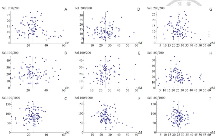
Figure 2 presents the scatter plots of the maxima of score test statistics of the posterior model under different selective proportions and marker densities. We can see

that the scatter points are more concentrated around the true position as the marker

becomes denser and the selective proportion gets more intense. Table 2 shows the score

test statistics and their thresholds of QTL mapping for full genotyping data, we found that

both of them become greater with denser markers. However, the powers to detect QTL

are slightly higher as marker becomes denser. For example, when the genetic effects are

set at 𝑎𝑎 = 1 , 𝑎𝑎 = 1, the score test statistics would be 11.34, 12.43 and 13.54, while their

thresholds would be 9.68, 10.35 and 10.99 respectively with marker densities being 20cM,

10cM and 5cM. There are increasing trends in both statistics and thresholds with the

denser markers. But the power to detect the QTL are stable at 58%, 61% and 63%,

respectively.

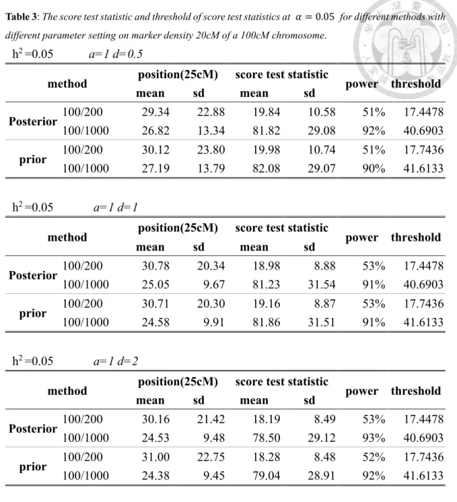
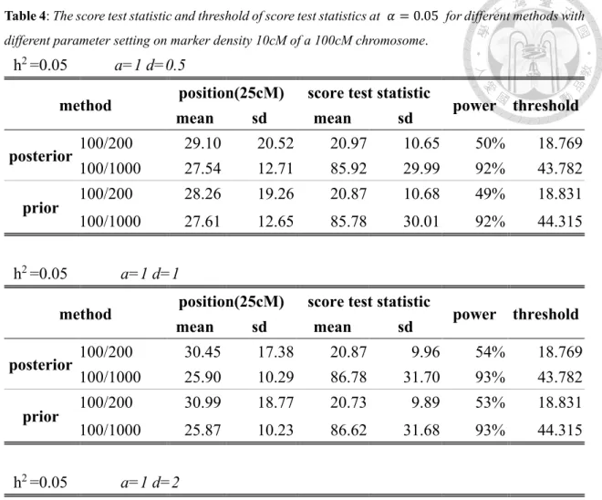
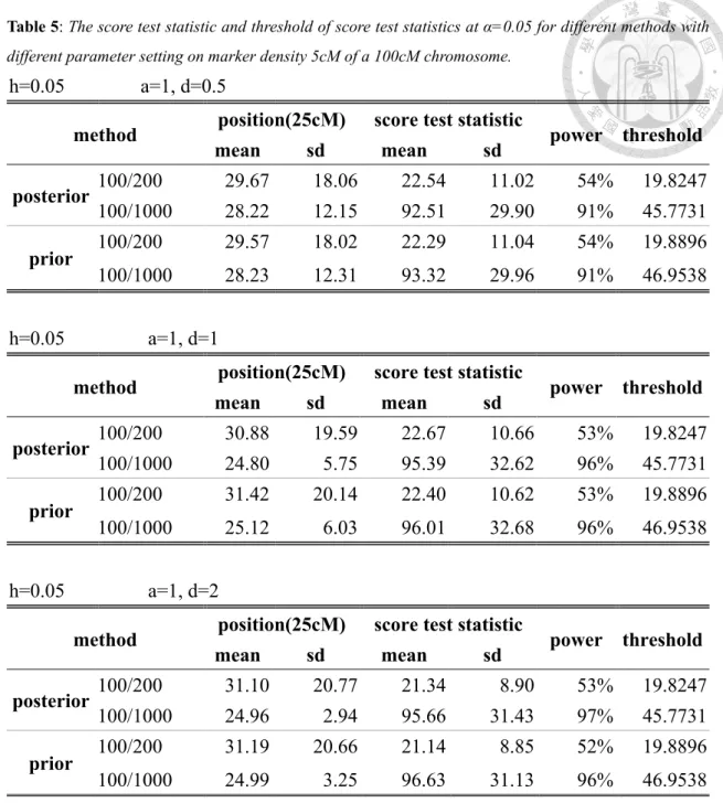
Tables 3 to 5 shows the score test statistics for both posterior and prior models as

well as their thresholds under marker densities 20cM, 10cM and 5cM. We can find that

the two score test statistics both increased when marker becomes denser and selective

proportion becomes more intense. For example, with posterior model, when selective

(22)

proportion is 50% (10%) and the marker densities are 20cM, 10cM and 5cM, the score

test statistics are 19.84 (81.82), 20.97 (85.92) and 22.54 (92.51), while the thresholds are

17.4478 (40.6906), 18.769 (43.782) and 19.8247 (45.7761). On the other hand, the score

test statistics for prior model are 19.98 (82.08), 20.87 (85.78) and 22.29 (93.32), while

the thresholds are 17.7436 (41.6133), 18.831 (44.315), 19.8896 (46.9538). Both score test

statistics for each model have the similar sizes and the similar thresholds.

In comparison with full genotyping data (Table 2), the score test statistics and their

thresholds under selective genotyping data (Tables 3-5) inflate. In addition, the results for

the two score test statistics (posterior and prior model) were similar. From Tables 2 to 5,

it is clear that the two models of score test statistics have similar performances. For

example, when genetic effects are (𝑎𝑎 = 1, 𝑎𝑎 = 0.5) and marker density is 10 cM, under

50% selective proportion, the score test statistics of posterior model (prior model) has a

mean of 20.97 (20.87) and the power to detect QTL is 50% (49%). When the selective

proportion is 10%, the score test statistics of the posterior model (prior model) and the

power for the posterior model (prior model) under the same settings become 85.92 (85.78)

and 92% (92%), respectively. It showed clearly that the more intense the selective

genotyping is, the greater the statistics inflate.

(23)

Figure 2: The scatter plots of the maximum score test statistics with a QTL at position 25cM on a 100-cM chromosome and genetic effect 𝑎𝑎 = 1, 𝑎𝑎 = 0.5 and ℎ²= 0.05. X-axis presents the marker positions (in cM). The marker density was 20cM (A-C), 10cM (D-F), 5cM (G-I) with the total population size 200, 200, 1000, and selective proportion 100%, 50%, 10% respectively. Each plots used 100 simulation replicates.

The dashed vertical lines indicate the QTL position (25 cM).

Table 2: the score test statistics and threshold of full genotyping data for different genetic effect and marker density 20cM, 10cM and 5cM on a 100cM chromosome.

h²=0.05 𝒂𝒂 = 𝟏𝟏 Sample size: 200/200

marker

distance d position(25cM) score test statistic

power threshold

mean sd mean sd

20cM

0.5 30.66 21.03 11.73 6.15 60%

9.6771

1 32.59 22.01 11.34 5.54 58%

2 31.68 23.04 11.04 5.46 57%

10cM

0.5 27.92 17.52 12.35 5.85 56%

10.351

1 30.60 16.94 12.43 5.84 61%

2 29.64 18.28 12.14 5.45 56%

5cM

0.5 30.98 19.09 13.23 6.08 57%

10.9863

1 30.76 17.85 13.54 6.27 63%

2 29.30 17.20 13.08 5.60 61%

(24)

Table 3: The score test statistic and threshold of score test statistics at 𝛼𝛼 = 0.05 for different methods with different parameter setting on marker density 20cM of a 100cM chromosome.

h²=0.05 a=1 d=0.5

method position(25cM) score test statistic

power threshold

Posterior 100/200 29.34 22.88 19.84 10.58 51% 17.4478 100/1000 26.82 13.34 81.82 29.08 92% 40.6903 prior 100/200 30.12 23.80 19.98 10.74 51% 17.7436 100/1000 27.19 13.79 82.08 29.07 90% 41.6133

h²=0.05 a=1 d=1

power threshold

Posterior 100/200 30.78 20.34 18.98 8.88 53% 17.4478 100/1000 25.05 9.67 81.23 31.54 91% 40.6903 prior 100/200 30.71 20.30 19.16 8.87 53% 17.7436 100/1000 24.58 9.91 81.86 31.51 91% 41.6133

h²=0.05 a=1 d=2

power threshold

Posterior 100/200 30.16 21.42 18.19 8.49 53% 17.4478 100/1000 24.53 9.48 78.50 29.12 93% 40.6903 prior 100/200 31.00 22.75 18.28 8.48 52% 17.7436 100/1000 24.38 9.45 79.04 28.91 92% 41.6133

(25)

Table 4: The score test statistic and threshold of score test statistics at 𝛼𝛼 = 0.05 for different methods with different parameter setting on marker density 10cM of a 100cM chromosome.

h²=0.05 a=1 d=0.5

power threshold

posterior 100/200 29.10 20.52 20.97 10.65 50% 18.769 100/1000 27.54 12.71 85.92 29.99 92% 43.782 prior 100/200 28.26 19.26 20.87 10.68 49% 18.831 100/1000 27.61 12.65 85.78 30.01 92% 44.315

h²=0.05 a=1 d=1

power threshold

posterior 100/200 30.45 17.38 20.87 9.96 54% 18.769 100/1000 25.90 10.29 86.78 31.70 93% 43.782 prior 100/200 30.99 18.77 20.73 9.89 53% 18.831 100/1000 25.87 10.23 86.62 31.68 93% 44.315

h²=0.05 a=1 d=2

power threshold

posterior 100/200 30.32 20.30 19.96 8.55 60% 18.769 100/1000 24.52 5.95 83.77 31.17 91% 43.782 prior 100/200 30.32 20.27 19.89 8.57 56% 18.831 100/1000 24.51 5.94 83.62 31.03 91% 44.315

(26)

Table 5: The score test statistic and threshold of score test statistics at α=0.05 for different methods with different parameter setting on marker density 5cM of a 100cM chromosome.

h=0.05 a=1, d=0.5

power threshold

posterior 100/200 29.67 18.06 22.54 11.02 54% 19.8247 100/1000 28.22 12.15 92.51 29.90 91% 45.7731 prior 100/200 29.57 18.02 22.29 11.04 54% 19.8896 100/1000 28.23 12.31 93.32 29.96 91% 46.9538

h=0.05 a=1, d=1

power threshold

posterior 100/200 30.88 19.59 22.67 10.66 53% 19.8247 100/1000 24.80 5.75 95.39 32.62 96% 45.7731 prior 100/200 31.42 20.14 22.40 10.62 53% 19.8896 100/1000 25.12 6.03 96.01 32.68 96% 46.9538

h=0.05 a=1, d=2

power threshold

posterior 100/200 31.10 20.77 21.34 8.90 53% 19.8247 100/1000 24.96 2.94 95.66 31.43 97% 45.7731 prior 100/200 31.19 20.66 21.14 8.85 52% 19.8896 100/1000 24.99 3.25 96.63 31.13 96% 46.9538

(27)

4 Conclusion and Discussion

In selective genotyping, only the individuals with upper and lower extreme trait

values are genotyped, while the remaining individuals are not. The score test statistic is

simple in derivation and computation in comparison to the likelihood approach. Based on

the posterior model proposed by Lee et al. (2013), which takes both genotyped and

ungenotyped individual into account in the analysis, we derived the score test statistic for

this posterior model for QTL mapping under selective genotyping. We also derived the

score test statistics for the model proposed by Xu and Vogl (2000) and Muranty and

Goffinet (1997) for comparisons. Moreover, we studied the threshold values of QTL

mapping in score test statistics of both models. The results show that the score test

statistics for posterior model and currently used model perform equally well under single-

QTL model. Given a significance level and a genome size, the threshold values are higher

in denser marker maps and extremer selective proportions when score test statistics are

used for QTL detection.

The results for full genotyping and for selective genotyping were compared. The test

statistics and thresholds from the maximum likelihood approach are similar, but these

results from their score test statistics have significant differences. The test statistics and

thresholds of score test statistics under selective genotyping are significantly inflated as

(28)

compared to those under full genotyping. However, the statistics (LRT) based on

maximum likelihood approach obtained by Lee et al. (2013) do not possess the trend of

enlargement as in the score test statistics under extremely selective genotyping. Reasons

for the inflation of statistics and thresholds for the score test statistics might be due to the

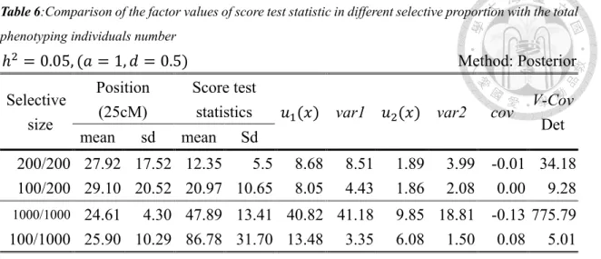
decrement of the variance when selection is more intense. Table 7 showed the mean

values of the score and their variances and covariance (u x₁

 

^、u x₂

 

and the variance- covariance matrix), we found that the score test statistic would raise under extremely

selective proportion and the variance of 𝜇𝜇₁(𝑥𝑥) and 𝜇𝜇₂(𝑥𝑥) would decrease with the

increasing number of total individuals. Moreover, the determinant of variance-covariance

matrix also becomes decreasing to enlarge the statistics gravely. However, the exact

reason for the inflations of the score test statistics and threshold values under selective

genotyping has not been well studied and deserves to be further investigated.

(29)

Table 6:Comparison of the factor values of score test statistic in different selective proportion with the total phenotyping individuals number

ℎ² = 0.05, (𝑎𝑎 = 1, 𝑎𝑎 = 0.5) Method: Posterior

Selective size

Position (25cM)

Score test

statistics 𝑢𝑢₁(𝑥𝑥) var1 𝑢𝑢₂(𝑥𝑥) var2 cov V-Cov mean sd mean Sd Det

200/200 27.92 17.52 12.35 5.5 8.68 8.51 1.89 3.99 -0.01 34.18 100/200 29.10 20.52 20.97 10.65 8.05 4.43 1.86 2.08 0.00 9.28

1000/1000 24.61 4.30 47.89 13.41 40.82 41.18 9.85 18.81 -0.13 775.79 100/1000 25.90 10.29 86.78 31.70 13.48 3.35 6.08 1.50 0.08 5.01 Each value based on 100 replicates with marker distance 10-cM along a 100-cM chromosome. (𝑢𝑢1(𝑥𝑥) and 𝑢𝑢2(𝑥𝑥) represent the score functions of a and d, var1 and var2 are the variance of 𝑢𝑢1(𝑥𝑥) and 𝑢𝑢₂(𝑥𝑥).)

(30)

In this thesis, we only considered the cases of a single QTL with small effects. As

shown in Tables 2 to 4, the results from the score test statistics of the currently used and

posterior models is similar because the frequencies of QTL genotypes in ungenotyped

individuals are close to the frequencies in the whole population ( 1/4、1/2 and 1/4 ) for

small QTL effect. Their differences will become more significant when the QTL has large

effects (not shown). Most quantitative traits are believed to be influenced by multiple

QTL and their interaction. In the cases of multiple QTL, the frequencies of multiple QTLs

genotypes among the ungenotyping individuals may deviate from the population

frequencies, and the differences between posterior model and currently used model might

become remarkable and is worth pursuing. In the future works, we intend to extend the

one-QTL posterior model to multiple-QTL posterior model for QTL detection when

selective genotyping is implemented in QTL experiments.

(31)

5 References

CHANG MYRON,N., R.WU, S.WU SAMUEL and G.CASELLA, 2009 Score Statistics for Mapping Quantitative Trait Loci, pp. 1 in Statistical Applications in Genetics and Molecular Biology.

COMMENGES, D., 1994 Robust genetic linkage analysis based on a score test of homogeneity: The weighted pairwise correlation statistic. Genetic Epidemiology 11: 189-200.

COMMENGES,D., and P.K.ANDERSEN, 1995 Score test of homogeneity for survival data.

Lifetime Data Analysis 1: 145-156.

COX,D.R., and D.V.HINKLEY, 1979 Theoretical statistics. Chapman & Hall/CRC.

DARVASI,A., and M.SOLLER, 1992 Selective genotyping for determination of linkage between a marker locus and a quantitative trait locus. Theoretical and Applied Genetics 85: 353-359.

DARVASI,A., A.WEINREB, V.MINKE, J.WELLER and M.SOLLER, 1993 Detecting marker- QTL linkage and estimating QTL gene effect and map location using a saturated genetic map. Genetics 134: 943-951.

DOERGE,R.W., and G.A.CHURCHILL, 1996 Permutation tests for multiple loci affecting a quantitative character. Genetics 142: 285-294.

DUDOIT,S., and T.P.SPEED, 2000 A score test for the linkage analysis of qualitative and quantitative traits based on identity by descent data from sib-pairs. Biostatistics 1:

1-26.

FEENSTRA,B., I.M.SKOVGAARD and K.W.BROMAN, 2006 Mapping Quantitative Trait Loci by an Extension of the Haley–Knott Regression Method Using Estimating Equations. Genetics 173: 2269-2282.

GELDERMANN, H., 1975 Investigations on inheritance of quantitative characters in animals by gene markers I. Methods. Theoretical and Applied Genetics 46: 319- 330.

GOLDSTEIN,D.R., S.DUDOIT and T.P.SPEED, 2001 Power and robustness of a score test for linkage analysis of quantitative traits using identity by descent data on sib pairs.

Genetic Epidemiology 20: 415-431.

GUO,Y.-T., 2011 進階回交族群之數量性狀基因座定位門檻值研究, pp. 1-55 in 臺灣大學農藝學研究所學位論文. 臺灣大學.

HALEY, C. S., and S. A. KNOTT, 1992 A simple regression method for mapping quantitative trait loci in line crosses using flanking markers. Heredity 69: 315-324.

HALEY,C. S., S.A. KNOTT and J. M. ELSEN, 1994 Mapping quantitative trait loci in

(32)

crosses between outbred lines using least squares. Genetics 136: 1195-1207.

JANSEN,R. C., 1993 Interval mapping of multiple quantitative trait loci. Genetics 135:

205-211.

JIANG,C., and Z.B.ZENG, 1995 Multiple trait analysis of genetic mapping for quantitative trait loci. Genetics 140: 1111-1127.

KAO,C.-H., 2000 On the Differences Between Maximum Likelihood and Regression Interval Mapping in the Analysis of Quantitative Trait Loci. Genetics 156: 855- 865.

KAO,C.-H., and Z.-B.ZENG, 1997 General Formulas for Obtaining the MLEs and the Asymptotic Variance- Covariance Matrix in Mapping Quantitative Trait Loci When Using the EM Algorithm. Biometrics 53: 653-665.

KAO, C.-H., Z.-B. ZENG and R. D. TEASDALE, 1999 Multiple Interval Mapping for Quantitative Trait Loci. Genetics 152: 1203-1216.

KAO,C. H., and H. A. HO, 2012 A score-statistic approach for determining threshold values in QTL mapping. Front Biosci (Elite Ed) 4: 2770-2782.

KNOTT,S.A., J.M.ELSEN and C.S.HALEY, 1996 Methods for multiple-marker mapping of quantitative trait loci in half-sib populations. Theoretical and Applied Genetics 93: 71-80.

KRUGLYAK, L., and E. S. LANDER, 1995 A nonparametric approach for mapping quantitative trait loci. Genetics 139: 1421-1428.

LANDER, E. S., and D. BOTSTEIN, 1989 Mapping mendelian factors underlying quantitative traits using RFLP linkage maps. Genetics 121: 185-199.

LEE,H.I., C.H.KAO and H.A.HO, 2013 A Novel Statistical Approach to QTL Mapping under Selective Genotyping: QTL Detection and Threshold Determination.

Unpublished.

LYNCH,M., and B.WALSH, 1998 Genetics and analysis of quantitative traits.

MATHER,K., 1941 Variation and selection of polygenic characters. Journal of Genetics 41: 159-193.

MURANTY,H., and B.GOFFINET, 1997 Selective Genotyping for Location and Estimation of the Effect of a Quantitative Trait Locus. Biometrics 53: 629-643.

OOIJEN, J., 1992 Accuracy of mapping quantitative trait loci in autogamous species.

Theoretical and Applied Genetics 84: 803-811.

PUTTER,H., L.A.SANDKUIJL and J.C. VAN HOUWELINGEN, 2002 Score test for detecting linkage to quantitative traits. Genetic Epidemiology 22: 345-355.

SEN, Ś., and G. A. CHURCHILL, 2001 A Statistical Framework for Quantitative Trait Mapping. Genetics 159: 371-387.

WANG, K., and J. HUANG, 2002 A Score-Statistic Approach for the Mapping of Quantitative-Trait Loci with Sibships of Arbitrary Size. The American Journal of

(33)

Human Genetics 70: 412-424.

WOLFRAM RESEARCH,I., 2012 Mathematica pp. Wolfram Research, Inc., Champaign, Illinois.

XU,S., and C.VOGL, 2000 Maximum likelihood analysis of quantitative trait loci under selective genotyping. Heredity 84: 525-537.

ZENG,Z. B., 1993 Theoretical basis for separation of multiple linked gene effects in mapping quantitative trait loci. Proceedings of the National Academy of Sciences 90: 10972-10976.

ZENG,Z.B., 1994 Precision mapping of quantitative trait loci. Genetics 136: 1457-1468.

(34)

6 Abbreviations

Abbreviations Term

QTL Quantitative trait loci

IM Interval mapping

LRT Likelihood ratio test

REG interval mapping Regression interval mapping

CIM Composite interval mapping

MIM Multiple interval mapping

應用分數檢定統計量於選擇性基因型試驗之數量性狀基因座定位研究

國立臺灣大學生物資源暨農學院農藝所生物統計組 碩士論文

National Taiwan University Master Thesis

應用分數檢定統計量於選擇性基因型試驗 之數量性狀基因座定位研究

Score Test Statistics for QTL Mapping under Selective Genotyping

房佑嬙

Yu-Chuang Fang

指導教授：高振宏 博士、廖振鐸 博士

Advisor: Chen-Hung Kao, Ph.D. & Chen-Tuo Liao, Ph.D.

中華民國 102 年 7 月

口試委員審定書

謝誌

中文摘要

ABSTRACT

Contents



















 



 

 

 

 

 

 





     

 

 

 

 





 

 



n



| g

|























 





 



 

 

  

  





 

 





 

 









國立臺灣大學生物資源暨農學院農藝所生物統計組碩士論文

應用分數檢定統計量於選擇性基因型試驗之數量性狀基因座定位研究

指導教授：高振宏博士、廖振鐸博士

^{| g}

^|

     ^{   } 