國立臺灣大學電機資訊學院資訊工程學系 碩士論文
Department of Computer Science and Information Engineering College of Electrical Engineering and Computer Science
National Taiwan University Master Thesis
針對彩色馬賽克影像的有效測邊器及其在直線偵測之 應用
Novel and Efficient Edge Detection on Color Mosaic Images with Application to Line Detection
王中周
Wang, Chung-Chou 指導教授:顏文明 副教授
傅楸善 教授
Advisor: Yan, Wen-Ming, Associate Prof.
Fuh, Chiou-Shann, Prof.
中華民國 97 年 6 月
June, 2008
i
國立臺灣大學碩士學位論文 口試委員會審定書
針對彩色馬賽克影像的有效測邊器及其在直線偵測之 應用
Novel and Efficient Edge Detection on Color Mosaic Images with Application to Line Detection
本論文係王中周君(R95922106)在國立臺灣大學資訊工 程學系完成之碩士學位論文,於民國 97 年 6 月 24 日承下列考 試委員審查通過及口試及格,特此證明
口試委員:
_________
(指導教授)
系 主 任
________
中文摘要
在這篇論文中,我們將提供一個新穎且有效的測邊器,在不進行解馬賽克的步驟 下,直接對馬賽克影像進行測邊,其方法是藉由結合Prewitt算子與馬賽克影像上 面的亮度估算技術,即可得到一對馬賽克影像上專用的測邊器。在傳統的非直接 測邊作法上,必須要先對馬賽克影像進行解馬賽克之步驟後,才可以在彩色影像
上面使用 Prewitt算子;兩個方法相互比較,我們所提出的直接測邊器的平均花費
時間快了48%。除此之外,其他的線性測邊器,例如Sobel算子與Marr-Hildreth算 子,亦可以透過類似的方法求得其馬賽克直接測邊器。
關鍵辭: 馬賽克影像, 解馬賽克演算法, 數位相機, 測邊, 測邊器, 直線增測,色彩濾 波陣列.
英文摘要
In this thesis, without demosaicing process, a new and efficient edge detector is presented for color mosaic images. Combining the Prewitt mask-pair and the lu- minance estimation technique for mosaic images, the required mask-pair for edge detection on the input mosaic image is derived first. Then, a novel edge detector for mosaic images is presented. Our proposed edge detector has the similar resulting edge map when compared with the indirect approach which first applies the demo- saicing process to the input mosaic image, and then runs the Prewitt edge detector on the demosaiced full color image. Based on some test mosaic images, experimen- tal results demonstrate that the average execution-time improvement ratio of our proposed edge detector over the indirect approach is about 48%. Our proposed results can also be applied to the other masks, e.g. the Sobel mask-pair and the Marr-Hildreth mask, for edge detection. Finally, the application to design a new line detection algorithm on mosaic images is investigated.
Keywords: Color filter array (CFA), Demosaicing algorithm, Digital cameras, Edge detection, Line detection, Mosaic images.
目 錄
口試委員會審定書 i
中文摘要 ii
英文摘要 iii
1 INTRODUCTION 1
2 PROPOSED EDGE DETECTOR FOR COLOR MOSAIC IMAGES 4 2.1 The Luminance Estimation Technique for Mosaic Images . . . 4 2.2 Proposed Prewitt- and Luminance Estimation-based Edge Detector . 6 2.3 Applications to derive Sobel Mask-pair and Marr-Hildreth Mask for
Mosaic Images . . . 10
3 PROPOSED LINE DETECTION ALGORITHM FOR COLOR MO-
SAIC IMAGES 15
4 EXPERIMENTAL RESULTS 18
5 CONCLUSIONS 29
參考書目 30
APPENDIX 1: THE DERIVATION FOR LUMINANCE ESTIMA-
TION 35
圖 目 錄
1.1 The Bayer CFA structure. . . 2
2.1 The 3× 3 single symmetric convolution mask. . . . 5
2.2 Four possible cases of 3× 3 mosaic subimages. (a) Case 1. (b) Case 2. (c) Case 3. (d) Case 4. . . 5
2.3 The 3× 3 luminance estimation mask. . . . 6
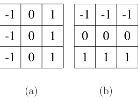
2.4 The 3 × 3 Prewitt mask-pair. (a) The horizontal mask. (b) The vertical mask. . . 7
2.5 The normalized PL-based mask-pair for mosaic images. (a) The hor- izontal mask. (b) The vertical mask. . . 10
2.6 The 3×3 Sobel mask-pair. (a) The horizontal mask. (b) The vertical mask. . . 10
2.7 The normalized SL-based mask-pair. (a) The horizontal mask. (b) The vertical mask. . . 12
2.8 The 11× 11 Marr-Hildreth mask. . . . 13
2.9 The normalized MHL-based mask. . . 14
3.1 The depiction of the alternative binary search test. . . 17
4.1 The four color test images for the mosaic edge detection. (a) Lady image. (b) Sailboats image. (c) Window image. (d) House image . . . 19
4.2 The down-sampled mosaic images. (a) mosaic Lady image. (b) mo- saic Sailboats image. (c) mosaic Window image. (d) mosaic House image . . . 19
4.3 The resultant edge maps. The resultant edge maps obtained by run- ning the indirect Prewitt-based approach on the mosaic images. (a) For Lady image. (b) For Sailboats image. (c) For Window image.
(d) For House image. The resultant edge maps obtained by running the proposed PL-based edge detector on the mosaic images. (e) For Lady image. (f) For Sailboats image. (g) For Window image. (h) For House image. . . 22 4.4 The resultant edge maps. The resultant edge maps obtained by run-
ning the indirect Sobel-based approach on the mosaic images. (a) For Lady image. (b) For Sailboats image. (c) For Window image.
(d) For House image. The resultant edge maps obtained by running the proposed SL-based edge detector on the mosaic images. (e) For Lady image. (f) For Sailboats image. (g) For Window image. (h) For House image. . . 23 4.5 The resultant edge maps. The resultant edge maps obtained by run-
ning the indirect Marr-Hildreth-based approach on the mosaic images.
(a) For Lady image. (b) For Sailboats image. (c) For Window image.
(d) For House image. The resultant edge maps obtained by running the proposed MHL-based edge detector on the mosaic images. (e) For Lady image. (f) For Sailboats image. (g) For Window image. (h) For House image. . . 24 4.6 The three test images for line detection. (a) Subsailboats image. (b)
Grating windows image. (c) Road image. . . 25 4.7 The obtained edge maps obtained by running the proposed SL-based
edge detector on the mosaic images. (a) For Subsailboats image. (b) For Grating windows image. (c) For Road image. . . 25 4.8 For Subsailboats image, the resulting detected lines obtained by using
(a) SHT, (b) RHT, (c) RLD, and (d) our proposed line detection algorithm. . . 26
4.9 For Grating windows image, the resulting detected lines obtained by using (a) SHT, (b) RHT, (c) RLD, and (d) our proposed line detection algorithm. . . 27 4.10 For Road image, the resulting detected lines obtained by using (a)
SHT, (b) RHT, (c) RLD, and (d) our proposed line detection algorithm. 28
表 目 錄
4.1 The average execution-time required in the indirect approach and our proposed approach for four test mosaic images. . . 20 4.2 The execution-time comparison among the four concerned line detec-
tion algorithms for three test mosaic images. . . 21
第 1 章
INTRODUCTION
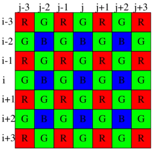
Recently, digital cameras have become more and more popular. In order to econo- mize the hardware cost, instead of using three CCD/CMOS sensors, most current digital cameras capture a color image with a single sensor array based on the Bayer color filter array (CFA) [3]. Based on the Bayer CFA structure, each pixel in the image has only one of the three primary colors, and this kind of images is called the mosaic image. The depiction of the Bayer CFA structure is illustrated in Fig.
1.1. Because the G (green) color channel is the most important factor to determine the luminance of the color image, half of the pixels in the Bayer CFA structure are assigned to the G channel to increase the image quality for the human visual system.
The R (red) and B (blue) color channels, which share the other half pixels in the Bayer CFA structure, are considered as the chrominance signals.
In the past several years, although several edge detectors [9, 14, 15, 18, 24, 26, 29, 31, 32, 33, 34] have been developed for full color images successfully, they cannot work well on mosaic images. Straightforwardly, when we want to perform edge detection on a mosaic image, we first adopt any one of existing demosaicing methods [1, 6, 7, 10, 11, 12, 17, 19, 20, 21, 22, 25, 30, 35, 36, 37, 38, 39] to the mosaic image, and then we perform edge detection on the demosaiced full color image to obtain the resultant edge map. Instead of using such an indirect approach, the main motivations of this thesis are two-fold: (1) presenting a new and efficient direct
B B R
B B
G G
R R
G G
R G G R
G B G B G
R G
G G G B
B G B G
G R G R G R
R
R G G G R
R R
R G G G R
i-3 i-2 i-1 i i+1 i+2 i+3
j-3 j-2 j-1 j j+1 j+2 j+3
Fig. 1.1: The Bayer CFA structure.
approach to perform edge detection on color mosaic images directly; (2) investigating the application to design a new line detection on color mosaic images directly.
In this thesis, without demosaicing process, a new and efficient edge detector is presented for color mosaic images. Combining the Prewitt mask-pair [27] and the luminance estimation technique for mosaic images [2], the required mask-pair for detecting edges on mosaic images directly is derived first. Then, our proposed edge detector is presented. To the best of our knowledge, this is the first time that such a novel edge detector on the color mosaic image domain is proposed. Based on some test mosaic images, experimental results demonstrate that our proposed edge detector has about 48% execution-time improvement ratio and has the similar resulting edge map when compared with the indirect approach. Our proposed results can be applied to the other masks, e.g. the Sobel mask-pair [16] and the Marr- Hildreth mask [23], for edge detection to speed up the computation. Finally, the application to design a new line detection algorithm on mosaic images is investigated.
The remainder of this thesis is organized as follows. In Chapter 2, combining the Prewitt mask-pair and the luminance estimation technique, our proposed edge detector for color mosaic images is presented, and then the utilizations to Sobel mask-pair and Marr-Hildreth mask are discussed. In Chapter 3, the application to design a novel line detection algorithm on mosaic images is investigated. In Chapter
4, some experiments are carried out to demonstrate the computation-saving advan- tage of our proposed edge detector on mosaic images. Some concluding remarks are addressed in Chapter 5.
第 2 章
PROPOSED EDGE DETECTOR FOR COLOR MOSAIC IMAGES
This chapter presents our proposed edge detector for color mosaic images. We first introduce the luminance estimation technique [2] which will be combined with the Prewitt mask-pair to derive two required masks for edge detection on mosaic images directly. The applications to the other masks, e.g. the Sobel mask-pair and the Marr-Hildreth mask also investigated. The main contribution of our proposed edge detector is that it has the similar resulting edge map as the one by using the indirect approach: first apply the demosaicing algorithm to the input mosaic image and then run the Prewitt edge detector on the demosaiced full color image, but has about 48% execution-time implement ratio.
2.1 The Luminance Estimation Technique for Mo- saic Images
In this section, the luminance estimation technique for mosaic images is introduced.
The luminance of a pixel with color value (R, G, B) is defined as L = 14(2G + R + B)
Fig. 2.1: The 3× 3 single symmetric convolution mask.
˥
˶˚
˶˥
˶˚
˶˕
˶˚
˶˥
˶˚
˶˥
˶˚
˶˥
˶˚
˶˕
˶˚
˶˕
˶˚
˶˥
˶˚
˶˕
˶˚
˶˕
˶˚
˶˥
˶˚
˶˕
˶˚
˶˕
˶˚
˶˕
˶˚
˶˥
˶˚
˶˥
˶˚
˶˕
˶˚
˶(a) (b) (c) (d)
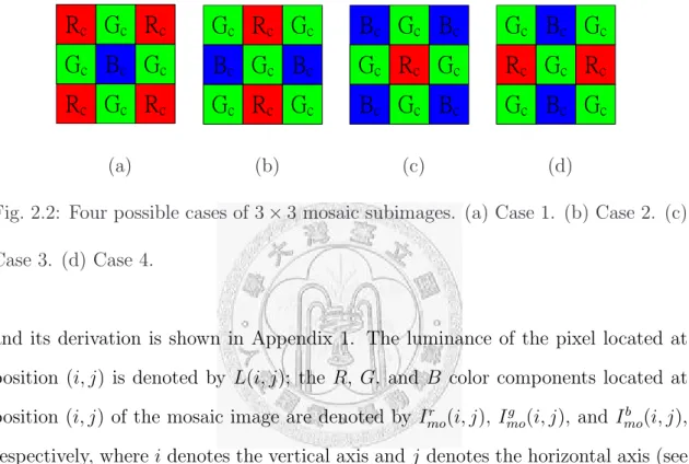
Fig. 2.2: Four possible cases of 3× 3 mosaic subimages. (a) Case 1. (b) Case 2. (c) Case 3. (d) Case 4.
and its derivation is shown in Appendix 1. The luminance of the pixel located at position (i, j) is denoted by L(i, j); the R, G, and B color components located at position (i, j) of the mosaic image are denoted by Imor (i, j), Imog (i, j), and Imob (i, j), respectively, where i denotes the vertical axis and j denotes the horizontal axis (see Fig. 1.1).
In order to estimate the luminance of the pixel at (i, j) in the mosaic image, a 3× 3 symmetric convolution mask as shown in Fig. 2.1 is used. Within a small smooth region of the mosaic image, the color values of R, G, and B components approximate to three different constants, i.e. Imor (i, j) ∼= Rc, Imog (i, j) ∼= Gc, and Imob (i, j) ∼= Bc. We consider all possible four cases of the 3× 3 mosaic subimage, and they are illustrated in Fig. 2.2(a)–(d), respectively. Because the 3× 3 mask in Fig. 2.1 is symmetric, we only need to consider Case 1 and Case 2 in Fig. 2.2.
First, each R channel of Case 1 and Case 2 is considered. After running the mask of Fig. 2.1 on the two 3× 3 mosaic subimages of Fig. 2.2(a) and Fig. 2.2(b), we have 4cRc = 2bRc. By the same argument, for the B channel, we have aBc = 2bBc.
˄˂˄ˉ ˄˂ˋ ˄˂˄ˉ
˄˂ˋ ˄˂ˇ ˄˂ˋ
˄˂˄ˉ ˄˂ˋ ˄˂˄ˉ
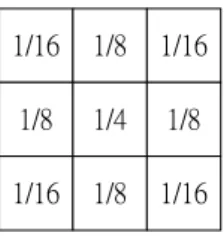
Fig. 2.3: The 3× 3 luminance estimation mask.
For normalizing the sum of nine coefficients in the mask, let a + 4b + 4c = 1. From 4c = 2b, a = 2b, and a + 4b + 4c = 1, it yields a = 14, b = 18, and c = 161. Thus, the luminance estimation mask can be determined and it is shown in Fig. 2.3. After running the the luminance estimation mask of Fig. 2.3 on the 3×3 mosaic subimage centered at position (i, j), the luminance L(i, j) can be obtained by
L(i, j) = 1 16
ImoC (i− 1, j − 1) + ImoC (i− 1, j + 1) +ImoC (i + 1, j− 1) + ImoC (i + 1, j + 1)
+2
ImoC (i− 1, j) + ImoC (i + 1, j) +ImoC (i, j− 1) + ImoC (i, j + 1)
+4ImoC (i, j)
(2.1)
where
ImoC (m, n) =
Imor (m, n) if m is odd and n is even Imog (m, n) if (m + n) is even
Imob (m, n) if m is even and n is odd
2.2 Proposed Prewitt- and Luminance Estimation- based Edge Detector
In this section, combining the Prewitt mask-pair and the luminance estimation technique, our proposed novel edge detector for mosaic images is presented.
-1 0 1 -1 0 1 -1 0 1
-1 -1 -1 0 0 0 1 1 1
(a) (b)
Fig. 2.4: The 3× 3 Prewitt mask-pair. (a) The horizontal mask. (b) The vertical mask.
Before presenting our proposed Prewitt- and luminance estimation-based (PL- based) edge detector, for completeness, we first introduce the Prewitt edge detector [27] for the luminance map. The 3×3 Prewitt mask-pair is illustrated in Fig. 2.4. It is known that given a luminance map, the luminance of the pixel located at position (i, j) is denoted by L(i, j). After running the Prewitt horizontal and vertical masks on the 3× 3 luminance submap centered at position (i, j), the horizontal response
∆H(i, j) and the vertical response ∆V (i, j) are given by
∆H(i, j) =
[
L(i− 1, j + 1) + L(i, j + 1) + L(i + 1, j + 1) ]
− [
L(i− 1, j − 1) + L(i, j − 1) + L(i + 1, j − 1) ]
∆V (i, j) =
[
L(i + 1, j− 1) + L(i + 1, j) + L(i + 1, j + 1) ]
− [
L(i− 1, j − 1) + L(i − 1, j) + L(i − 1, j + 1) ]
(2.2)
In order to make the Prewitt edge detector feasible for mosaic images to ex- tract more accurate edge information, the luminance estimation technique could be plugged into the Prewitt edge detector. Combining Eq. (2.1) and Eq. (2.2), the two kernel responses used in our proposed edge detector for mosaic images can be
obtained by the following derivations:
∆H(i, j) =
[
L(i− 1, j + 1) + L(i, j + 1) + L(i + 1, j + 1) ]
− [
L(i− 1, j − 1) + L(i, j − 1) + L(i + 1, j − 1) ]
= 1 16
ImoC (i− 2, j + 2) + ImoC (i + 2, j + 2)
−ImoC (i− 2, j − 2) − ImoC (i + 2, j− 2)
+2
ImoC (i− 2, j + 1) + ImoC (i + 2, j + 1)
−ImoC (i− 2, j − 1) − ImoC (i + 2, j− 1)
+3
ImoC (i− 1, j + 2) + ImoC (i + 1, j + 2)
−ImoC (i− 1, j − 2) − ImoC (i + 1, j− 2)
+4 [
ImoC (i, j + 2)− ImoC (i, j− 2) ]
+6
ImoC (i− 1, j + 1) + ImoC (i + 1, j + 1)
−ImoC (i− 1, j − 1) − ImoC (i + 1, j− 1)
+8 [
ImoC (i, j + 1)− ImoC (i, j− 1) ]
(2.3)
∆V (i, j) =
[
L(i + 1, j− 1) + L(i + 1, j) + L(i + 1, j + 1) ]
− [
L(i− 1, j − 1) + L(i − 1, j) + L(i − 1, j + 1) ]
= 1 16
ImoC (i + 2, j − 2) + ImoC (i + 2, j + 2)
−ImoC (i− 2, j − 2) − ImoC (i− 2, j + 2)
+2
ImoC (i + 1, j− 2) + ImoC (i + 1, j + 2)
−ImoC (i− 1, j − 2) − ImoC (i− 1, j + 2)
+3
ImoC (i + 2, j− 1) + ImoC (i + 2, j + 1)
−ImoC (i− 2, j − 1) − ImoC (i− 2, j + 1)
+4 [
ImoC (i + 2, j)− ImoC (i− 2, j) ]
+6
ImoC (i + 1, j− 1) + ImoC (i + 1, j + 1)
−ImoC (i− 1, j − 1) − ImoC (i− 1, j + 1)
+8 [
ImoC (i + 1, j)− ImoC (i− 1, j) ]
(2.4)
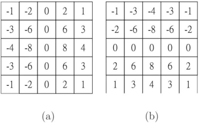
By Eq. (2.3) and Eq. (2.4), the PL-based mask-pair can be followed easily. For saving computational effort, the coefficients in the derived mask–pair are normalized to integers, and the normalized PL-based mask-pair for mosaic images is depicted in Fig. 2.5.
After running the above proposed PL-based mask-pair on the 5×5 mosaic subim- age centered at position (i, j), the horizontal response ∆H(i, j) and the vertical re- sponse ∆V (i, j) can be obtained. Based on the values of ∆H(i, j) and ∆V (i, j), the gradient magnitude∇GM(i, j) and the direction of variation θ(i, j) can be computed by∇GM(i, j) =√
[∆H(i, j)]2+ [∆V (i, j)]2 and θ(i, j) = tan−1 ∆V (i,j)
∆H(i,j), respectively.
Finally, the obtained∇GM(i, j) and θ(i, j) can be used to detect edges on mosaic images directly. If the value of∇GM(i, j) is larger than the specified threshold, the pixel at location (i, j) in the mosaic image is treated as an edge pixel with direction θ(i, j); otherwise it is a non–edge pixel.
ˀ˄ ˀ˅ ˃ ˅ ˄ ˀˆ ˀˉ ˃ ˉ ˆ ˀˇ ˀˋ ˃ ˋ ˇ ˀˆ ˀˉ ˃ ˉ ˆ ˀ˄ ˀ˅ ˃ ˅ ˄
ˀ˄ ˀˆ ˀˇ ˀˆ ˀ˄
ˀ˅ ˀˉ ˀˋ ˀˉ ˀ˅
˃ ˃ ˃ ˃ ˃
˅ ˉ ˋ ˉ ˅
˄ ˆ ˇ ˆ ˄
(a) (b)
Fig. 2.5: The normalized PL-based mask-pair for mosaic images. (a) The horizontal mask. (b) The vertical mask.
-1 0 1 -2 0 2 -1 0 1
-1 -2 -1 0 0 0 1 2 1
(a) (b)
Fig. 2.6: The 3× 3 Sobel mask-pair. (a) The horizontal mask. (b) The vertical mask.
2.3 Applications to derive Sobel Mask-pair and Marr-Hildreth Mask for Mosaic Images
Following the results of the last section, the derivations to Sobel mask-pair [16]
and Marr-Hildreth mask [23] for mosaic images are presented in this section. We first present the combination of the Sobel mask-pair and the luminance estimation technique, and then the combination of the Marr-Hildreth mask and the luminance estimation technique is presented.
By the same argument of the Prewitt mask-pair, after running the Sobel mask- pair as shown in Fig. 2.6 on the 3× 3 luminance submap centered at position (i, j),
the horizontal response ∆H(i, j) and the vertical response ∆V (i, j) are given by
∆H(i, j) =
[
L(i− 1, j + 1) + 2L(i, j + 1) + L(i + 1, j + 1) ]
− [
L(i− 1, j − 1) + 2L(i, j − 1) + L(i + 1, j − 1) ]
∆V (i, j) =
[
L(i + 1, j − 1) + 2L(i + 1, j) + L(i + 1, j + 1) ]
− [
L(i− 1, j − 1) + 2L(i − 1, j) + L(i − 1, j + 1) ]
(2.5)
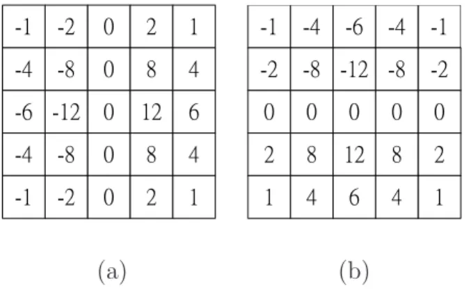
Then, combining Eq. (2.1) and Eq. (2.5), the Sobel- and luminance estimation- based (SL-based) mask-pair can be obtained by the following derivations:
∆H(i, j) =
[
L(i− 1, j + 1) + 2L(i, j + 1) + L(i + 1, j + 1) ]
− [
L(i− 1, j − 1) + 2L(i, j − 1) + L(i + 1, j − 1) ]
= 1 16
ImoC (i− 2, j + 2) + ImoC (i + 2, j + 2)
−ImoC (i− 2, j − 2) − ImoC (i + 2, j− 2)
+2
ImoC (i− 2, j + 1) + ImoC (i + 2, j + 1)
−ImoC (i− 2, j − 1) − ImoC (i + 2, j− 1)
+4
ImoC (i− 1, j + 2) + ImoC (i + 1, j + 2)
−ImoC (i− 1, j − 2) − ImoC (i + 1, j− 2)
+6 [
ImoC (i, j + 2)− ImoC (i, j− 2) ]
+8
ImoC (i− 1, j + 1) + ImoC (i + 1, j + 1)
−ImoC (i− 1, j − 1) − ImoC (i + 1, j− 1)
+12 [
ImoC (i, j + 1)− ImoC (i, j− 1) ]
ˀ˄ ˀ˅ ˃ ˅ ˄ ˀˇ ˀˋ ˃ ˋ ˇ ˀˉ ˀ˄˅ ˃ ˄˅ ˉ ˀˇ ˀˋ ˃ ˋ ˇ ˀ˄ ˀ˅ ˃ ˅ ˄
ˀ˄ ˀˇ ˀˉ ˀˇ ˀ˄
ˀ˅ ˀˋ ˀ˄˅ ˀˋ ˀ˅
˃ ˃ ˃ ˃ ˃
˅ ˋ ˄˅ ˋ ˅
˄ ˇ ˉ ˇ ˄
(a) (b)
Fig. 2.7: The normalized SL-based mask-pair. (a) The horizontal mask. (b) The vertical mask.
∆V (i, j) =
[
L(i + 1, j − 1) + 2L(i + 1, j) + L(i + 1, j + 1) ]
− [
L(i− 1, j − 1) + 2L(i − 1, j) + L(i − 1, j + 1) ]
= 1 16
ImoC (i + 2, j− 2) + ImoC (i + 2, j + 2)
−ImoC (i− 2, j − 2) − ImoC (i− 2, j + 2)
+2
ImoC (i + 1, j − 2) + ImoC (i + 1, j + 2)
−ImoC (i− 1, j − 2) − ImoC (i− 1, j + 2)
+4
ImoC (i + 2, j − 1) + ImoC (i + 2, j + 1)
−ImoC (i− 2, j − 1) − ImoC (i− 2, j + 1)
+6 [
ImoC (i + 2, j)− ImoC (i− 2, j) ]
+8
ImoC (i + 1, j − 1) + ImoC (i + 1, j + 1)
−ImoC (i− 1, j − 1) − ImoC (i− 1, j + 1)
+12 [
ImoC (i + 1, j)− ImoC (i− 1, j) ]
Further, we normalize the coefficients in the derived SL-based masks. The normal- ized horizontal mask and vertical mask are illustrated in Fig. 2.7.
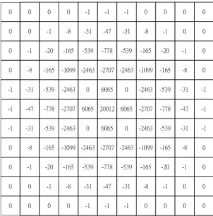
Besides the Prewitt mask and the Sobel mask, the Marr-Hildreth mask is also a
× 11 Marr-Hildreth mask is illustrated in Fig.
˃ ˃ ˃ ˃ ˀ˄ ˀ˄
˃ ˃ ˀ˄ ˀˋ ˀˆ˄ ˀˇˊ
˃ ˀ˄ ˀ˅˃ ˀ˄ˉˈ ˀˈˆˌ ˀˊˊˋ
˃ ˀˋ ˀ˄ˉˈ ˀ˄˃ˌˌ ˀ˅ˇˉˆ ˀ˅ˊ˃ˊ
ˀ˄ ˀˆ˄ ˀˈˆˌ ˀ˅ˇˉˆ ˃ ˉ˃ˉˈ
ˀ˄ ˀˇˊ ˀˊˊˋ ˀ˅ˊ˃ˊ ˉ˃ˉˈ ˅˃˃˄˅
ˀ˄
ˀˆ˄
ˀˈˆˌ ˀ˅ˇˉˆ
˃ ˉ˃ˉˈ
˃ ˀˋ ˀ˄ˉˈ ˀ˄˃ˌˌ ˀ˅ˇˉˆ ˀ˅ˊ˃ˊ
˃ ˀ˄
ˀ˅˃
ˀ˄ˉˈ ˀˈˆˌ ˀˊˊˋ
˃
˃ ˀ˄
ˀˋ ˀˆ˄
ˀˇˊ
˃
˃
˃
˃ ˀ˄
ˀ˄
ˀ˄ ˀˆ˄ ˀˈˆˌ ˀ˅ˇˉˆ ˃ ˉ˃ˉˈ ˃ ˀ˅ˇˉˆ ˀˈˆˌ ˀˆ˄ ˀ˄
˃ ˀˋ ˀ˄ˉˈ ˀ˄˃ˌˌ ˀ˅ˇˉˆ ˀ˅ˊ˃ˊ ˀ˅ˇˉˆ ˀ˄˃ˌˌ ˀ˄ˉˈ ˀˋ ˃
˃ ˀ˄ ˀ˅˃ ˀ˄ˉˈ ˀˈˆˌ ˀˊˊˋ ˀˈˆˌ ˀ˄ˉˈ ˀ˅˃ ˀ˄ ˃
˃ ˃ ˀ˄ ˀˋ ˀˆ˄ ˀˇˊ ˀˆ˄ ˀˋ ˀ˄ ˃ ˃
˃ ˃ ˃ ˃ ˀ˄ ˀ˄ ˀ˄ ˃ ˃ ˃ ˃
Fig. 2.8: The 11× 11 Marr-Hildreth mask.
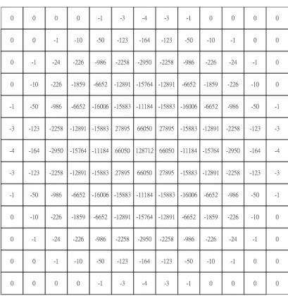
2.8. The response ∆2M H(i, j) can be obtained by running the 11×11 Marr-Hildreth mask on the 11×11 luminance submap centered at location (i, j), too. Following the same way mentioned above, the luminance estimation technique could be plugged into the Marr-Hildreth edge detector, and then by normalizing the coefficients in the derived mask. The normalized Marr-Hildreth- and luminance estimation-based (MHL-based) mask is illustrated in Fig. 2.9.
After running the MHL-based mask on the 13×13 mosaic subimage, the response
∆2M H(i, j) can be obtained. When the zero-crossing condition, i.e. ∆2M H(i− 1, j)× ∆2M H(i + 1, j) < 0 or ∆2M H(i, j− 1) × ∆2M H(i, j + 1) < 0, happens and the absolute value of the relevant difference, i.e. |∆2M H(i− 1, j) − ∆2M H(i + 1, j)| or|∆2M H(i, j−1)−∆2M H(i, j + 1)|, is larger than the specific threshold, the pixel at location (i, j) in the mosaic image can be treated as an edge pixel; otherwise it is a non–edge pixel.
ˀˆ ˀ˄˅ˆ ˀ˅˅ˈˋ ˀ˄˅ˋˌ˄ ˀ˄ˈˋˋˆ ˅ˊˋˌˈ ˉˉ˃ˈ˃
ˀˇ ˀ˄ˉˇ ˀ˅ˌˈ˃ ˀ˄ˈˊˉˇ ˀ˄˄˄ˋˇ ˉˉ˃ˈ˃ ˄˅ˋˊ˄˅
˃ ˃ ˃ ˃ ˀ˄ ˀˆ ˀˇ
˃ ˃ ˀ˄ ˀ˄˃ ˀˈ˃ ˀ˄˅ˆ ˀ˄ˉˇ
˃ ˀ˄ ˀ˅ˇ ˀ˅˅ˉ ˀˌˋˉ ˀ˅˅ˈˋ ˀ˅ˌˈ˃
˃ ˀ˄˃ ˀ˅˅ˉ ˀ˄ˋˈˌ ˀˉˉˈ˅ ˀ˄˅ˋˌ˄ ˀ˄ˈˊˉˇ
ˀ˄ ˀˈ˃ ˀˌˋˉ ˀˉˉˈ˅ ˀ˄ˉ˃˃ˉ ˀ˄ˈˋˋˆ ˀ˄˄˄ˋˇ
ˀˆ ˀ˄˅ˆ ˀ˅˅ˈˋ ˀ˄˅ˋˌ˄ ˀ˄ˈˋˋˆ ˅ˊˋˌˈ ˉˉ˃ˈ˃
ˀ˄ ˀˈ˃ ˀˌˋˉ ˀˉˉˈ˅ ˀ˄ˉ˃˃ˉ ˀ˄ˈˋˋˆ ˀ˄˄˄ˋˇ
˃ ˀ˄˃ ˀ˅˅ˉ ˀ˄ˋˈˌ ˀˉˉˈ˅ ˀ˄˅ˋˌ˄ ˀ˄ˈˊˉˇ
˃ ˀ˄ ˀ˅ˇ ˀ˅˅ˉ ˀˌˋˉ ˀ˅˅ˈˋ ˀ˅ˌˈ˃
˃ ˃ ˀ˄ ˀ˄˃ ˀˈ˃ ˀ˄˅ˆ ˀ˄ˉˇ
˃ ˃ ˃ ˃ ˀ˄ ˀˆ ˀˇ
˅ˊˋˌˈ
ˉˉ˃ˈ˃
ˀˆ
ˀ˄˅ˆ
ˀ˅˅ˈˋ
ˀ˄˅ˋˌ˄
ˀ˄ˈˋˋˆ
˅ˊˋˌˈ
ˀ˄ˈˋˋˆ
ˀ˄˅ˋˌ˄
ˀ˅˅ˈˋ
ˀ˄˅ˆ
ˀˆ ˀ˄ˈˋˋˆ
ˀ˄˄˄ˋˇ ˀ˄
ˀˈ˃
ˀˌˋˉ
ˀˉˉˈ˅
ˀ˄ˉ˃˃ˉ
ˀ˄ˈˋˋˆ
ˀ˄ˉ˃˃ˉ
ˀˉˉˈ˅
ˀˌˋˉ
ˀˈ˃
ˀ˄
ˀ˄˅ˋˌ˄
ˀ˄ˈˊˉˇ
˃
ˀ˄˃
ˀ˅˅ˉ
ˀ˄ˋˈˌ
ˀˉˉˈ˅
ˀ˄˅ˋˌ˄
ˀˉˉˈ˅
ˀ˄ˋˈˌ
ˀ˅˅ˉ
ˀ˄˃
˃ ˀ˅˅ˈˋ
ˀ˅ˌˈ˃
˃
ˀ˄
ˀ˅ˇ
ˀ˅˅ˉ
ˀˌˋˉ
ˀ˅˅ˈˋ
ˀˌˋˉ
ˀ˅˅ˉ
ˀ˅ˇ
ˀ˄
˃ ˀ˄˅ˆ
ˀ˄ˉˇ
˃
˃
ˀ˄
ˀ˄˃
ˀˈ˃
ˀ˄˅ˆ
ˀˈ˃
ˀ˄˃
ˀ˄
˃
˃ ˀˆ
ˀˇ
˃
˃
˃
˃
ˀ˄
ˀˆ
ˀ˄
˃
˃
˃
˃
Fig. 2.9: The normalized MHL-based mask.
第 3 章
PROPOSED LINE DETECTION ALGORITHM FOR COLOR
MOSAIC IMAGES
In this chapter, our proposed novel line detection algorithm, which uses the edge map obtained in Chapter 2 to be the input image, is presented. Our proposed line detection algorithm consists of the following four steps, namely the initialization, the candidate line determination, the voting process, and the true line determination.
Stage 1: (Initialization)
We have set of edge pixels E = {em = (im, jm)|m ∈ {1, 2, . . . , N}} where en = (in, jn) denotes the n-th edge pixel in the set E and the edge pixel en locates at the position (in, jn); N denotes the number of the edge pixels in the set E. Then, the failure counter is denoted by Cf and it is initially set to zero. Three thresholds, Tcl, Tf, and Ttl are used where Tcl denote the repeating times of the alternative binary search test which will be presented in Step 2; Tf denotes the number of successive failures that we can tolerate; Ttl denotes the least edge pixels which a true line should
include. Moreover, the voting set V←−→exey is used to collect the edge pixels which are on the candidate line ←→exey, and it is set to V←−→exey =∅, initially.
Stage 2: (The candidate line determination)
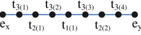
First, two edge pixels ex = (ix, jx) and ey = (iy, jy) are randomly picked out form the set E and then ←→exey is set to be an initial line. Then, the alternative binary search test is used to determine whether the initial line
←→exey is a candidate line or not. Fig. 3.1 illustrates the depiction of the alternative binary search test. After picking ex = (ix, jx) and ey = (iy, jy) out, the pixel t1(1)= (i1(1), j1(1)), which is the midpoint of the line segment exey, i.e. (i1(1), j1(1)) = (ix+i2 y,jx+j2 y), is examined whether it is an edge pixel or not. If t1(1) is an edge pixel, the two points t2(1) and t2(2), which are the midpoints of the line segments ext1(1) and t1(1)ey, respectively, are examined whether they are all edge pixels. If the above condition holds, the four points t3(1)–t3(4) are picked to examine. The alternative binary search test is repeated until the repeating times are over the threshold Tcl. Then, the line ←→exey is determined to be a candidate line and go to Step 3.
Otherwise, the line ←→exey is not a candidate line and perform Cf = Cf + 1.
If Cf > Tf, then stop; otherwise, go to Step 2.
Stage 3: (The voting process)
Bresenham’s line algorithm [4] is utilized to plot the path ←→exey and to determine which edge pixels in the edge map is on ←→exey. If the edge pixel ev = (iv, jv) is on the plotted path ←→exey, we add ev = (iv, jv) into the voting set V←−→exey, i.e. V←−→exey ={ev = (iv, jv)| ev ∈ E, ev on the line ←→exey}.
Stage 4: (The true line determination)
If the number of edge pixels in the voting set V←−→exey is greater than or equal to the threshold Ttl, i.e. |V←−→exey| ≥ Ttl, the candidate line ←→exey is a true line.
We take the edge pixels in the voting set V←−→exey out of E, i.e. E = E−V←−→exey.
∅ and C
e
xt
2(1)t
1(1)t
2(2)e
yt
3(1)t
3(2)t
3(3)t
3(4)Fig. 3.1: The depiction of the alternative binary search test.
as a false line and perform Cf = Cf+ 1. If Cf > Tf, then stop; otherwise, set V←−→exey =∅ and go to Step 2.
第 4 章
EXPERIMENTAL RESULTS
In this chapter, based on some test images, experimental results demonstrate that our proposed edge detector to detect edges on mosaic images directly has the similar edge detection effect but has better time performance when compared with the indirect approach. Besides, some experiments are carried out to demonstrate the computation-saving benefit of our proposed line detection algorithm when running it on the edge map obtained by our proposed edge detector for mosaic images.
For convenience, the indirect approach which uses color Prewitt edge detector is called the indirect Prewitt-based approach, so as that of the indirect Sobel-based approach and the indirect Marr-Hildreth-based approach. The concerned algorithms are implemented on the IBM compatible computer with Intel Core 2 Duo CPU @ 1.6GHz and 1GB RAM. The operating system used is MS-Windows XP and the program developing environment is Borland C++ Builder 6.0. Our program has been uploaded in [43].
Figs. 4.1(a)–(d) illustrate the four color test images, namely Lady image, Sail- boats image, Window image, and House image, respectively, for the mosaic edge detection. In our experiments, the four color test images are first down-sampled to obtain the mosaic images as shown in Figs. 4.2(a)–(d), respectively.
Figs. 4.3(a)–(d) and Figs. 4.3(e)–(h) illustrate the resultant edge maps ob- tained by running the indirect Prewitt-based approach and our proposed PL-based
(a) (b) (c) (d) Fig. 4.1: The four color test images for the mosaic edge detection. (a) Lady image.
(b) Sailboats image. (c) Window image. (d) House image
(a) (b) (c) (d)
Fig. 4.2: The down-sampled mosaic images. (a) mosaic Lady image. (b) mosaic Sailboats image. (c) mosaic Window image. (d) mosaic House image
edge detector, respectively, on four test mosaic images as shown in Fig. 4.2. As a postprocessing, the nonmaxima suppression rule [5] is adopted in the implemen- tation. The resultant edge maps obtained by the indirect Sobel-based approach and our proposed SL-based edge detector are illustrated in Figs. 4.4(a)–(d) and Figs. 4.4(e)–(h), respectively. Figs. 4.5(a)–(d) and Figs. 4.5(e)–(h) illustrate the resultant edge maps obtained by the indirect Marr-Hildreth-based approach and ourproposed MHL-based edge detector, respectively. Table 4.1 demonstrates the average execution-time required in the indirect edge detection approach and our proposed direct approach for four test mosaic images where the time unit is second.
表 4.1: The average execution-time required in the indirect approach and our pro- posed approach for four test mosaic images.
Indirect approach Our proposed approach Improvement ratio
Prewitt 0.226(s) 0.118(s) 47.79%
Sobel 0.240(s) 0.118(s) 50.83%
Marr-Hildreth 1.289(s) 0.586(s) 54.54%
According to Figs. 4.3–4.5 and Table 4.1, experimental results demonstrate that our proposed edge detector to detect edges on mosaic image directly has the similar edge detection results when compared with the indirect approach; however, the av- erage execution-time improvement-ratios of our proposed PL-based, SL-based, and MHL-based edge detectors over the corresponding indirect approaches are 47.79%, 50.83%, and 54.54%, respectively.
Further, some line detection results are given to demonstrate that our proposed line detection algorithm has better computational performance when compared with Standard Hough transform (SHT) [13, 28], Randomized Hough transform (RHT) [40, 41], and Randomized line detection algorithm (RLD) [8]. Figs. 4.6(a)–(c) illustrate the three color test images, namely Subsailboats image, Grating windows image, and Road image, respectively, for the line detection. Among the three test images, Fig. 4.6(a) is the subimage cut from Fig. 4.1(b) because it has more line patterns. In our experiments, the three color test images are first down-sampled to obtain the mosaic images, and then running our proposed SL-based edge detector on the mosaic images. Figs. 4.7(a)–(c) illustrate the obtained edge maps.
For the three edge maps in Figs. 4.7(a)–(c), after running SHT, RHT, RLD and our proposed line detection algorithm, the resulting detected lines are shown in Figs. 4.8–4.10, respectively. For three test mosaic images, Table 4.2 illustrates
表 4.2: The execution-time comparison among the four concerned line detection algorithms for three test mosaic images.
Algorithm SHT RHT RLD Proposed
Subsailboats image 0.143(s) 0.126(s) 0.072(s) 0.064(s) Grating windows image 0.137(s) 0.114(s) 0.088(s) 0.060(s) Road image 0.136(s) 0.106(s) 0.046(s) 0.027(s) Average 0.139(s) 0.115(s) 0.069(s) 0.050(s)
the execution-time comparison among the four concerned line detection algorithms.
From Table 4.2, the average execution-time of SHT, RHT, RLD, and our pro- posed algorithm are 0.139s, 0.115s, 0.069s, and 0.050s, respectively. In average, the execution-time improvement ratio of our proposed algorithm over SHT, RHT, and RLD are 64.03% (0.1390.139−0.050×100%), 56.52% (= 0.1150.115−0.050×100%), and 27.54%
(= 0.069−0.050
0.069 × 100%), respectively.
Finally, according to the above experimentations and discussions, it is observed that our proposed edge detector for mosaic images has better computational per- formance than the indirect approach and our proposed line detection algorithm has the best computational performance among the four concerned line detection algo- rithms. Thus, combining the proposed edge detector and the proposed line detection algorithm is the most efficient approach to detect the lines from mosaic images.
(a) (b) (c) (d)
(e) (f) (g) (h)
Fig. 4.3: The resultant edge maps. The resultant edge maps obtained by running the indirect Prewitt-based approach on the mosaic images. (a) For Lady image. (b) For Sailboats image. (c) For Window image. (d) For House image. The resultant edge maps obtained by running the proposed PL-based edge detector on the mosaic images. (e) For Lady image. (f) For Sailboats image. (g) For Window image. (h) For House image.
(a) (b) (c) (d)
(e) (f) (g) (h)
Fig. 4.4: The resultant edge maps. The resultant edge maps obtained by running the indirect Sobel-based approach on the mosaic images. (a) For Lady image. (b) For Sailboats image. (c) For Window image. (d) For House image. The resultant edge maps obtained by running the proposed SL-based edge detector on the mosaic images. (e) For Lady image. (f) For Sailboats image. (g) For Window image. (h) For House image.
(a) (b) (c) (d)
(e) (f) (g) (h)
Fig. 4.5: The resultant edge maps. The resultant edge maps obtained by running the indirect Marr-Hildreth-based approach on the mosaic images. (a) For Lady image. (b) For Sailboats image. (c) For Window image. (d) For House image. The resultant edge maps obtained by running the proposed MHL-based edge detector on the mosaic images. (e) For Lady image. (f) For Sailboats image. (g) For Window image. (h) For House image.
(a) (b) (c)
Fig. 4.6: The three test images for line detection. (a) Subsailboats image. (b) Grating windows image. (c) Road image.
(a) (b) (c)
Fig. 4.7: The obtained edge maps obtained by running the proposed SL-based edge detector on the mosaic images. (a) For Subsailboats image. (b) For Grating windows image. (c) For Road image.
(a) (b)
(c) (d)
Fig. 4.8: For Subsailboats image, the resulting detected lines obtained by using (a) SHT, (b) RHT, (c) RLD, and (d) our proposed line detection algorithm.
(a) (b)
(c) (d)
Fig. 4.9: For Grating windows image, the resulting detected lines obtained by using (a) SHT, (b) RHT, (c) RLD, and (d) our proposed line detection algorithm.
(a) (b)
(c) (d)
Fig. 4.10: For Road image, the resulting detected lines obtained by using (a) SHT, (b) RHT, (c) RLD, and (d) our proposed line detection algorithm.
第 5 章
CONCLUSIONS
Without demosaicing process, a new and efficient edge detector has been presented for color mosaic images directly. Combining the Prewitt mask-pair and the lumi- nance estimation technique for mosaic images, the mask-pair for edge detection on the input mosaic image is derived first. Then, a novel edge detection algorithm for mosaic images is proposed. Experimental results demonstrate that the proposed edge detector to detect edges on mosaic images directly has the similar edge de- tection results when compared with the indirect approach which first applies the demosaicing process to the input mosaic image, and then runs the Prewitt edge detector on the demosaiced full color image; however, the average execution-time improvement-ratio of our proposed edge detector over the indirect approach is about 48%. Our proposed results can be applied to the other masks, e.g. the Sobel mask- pair and the Marr-Hildreth mask, for edge detection. Finally, the application to design a new line detection algorithm on mosaic images is investigated. Based on some test images, our proposed line detection algorithm has better computational performance when compared with SHT [13, 28], RHT [40, 41], and RLD [8]. Thus, according to the experimentations and discussions, combining the proposed edge detector and the proposed line detection algorithm is the most efficient approach to detect the lines from mosaic images.
參 考 書 目
[1] J. E. Adams and J. F. Hamilton, “Adaptive color plan interpolation in single sensor color electric camera,” U.S. Patent 5 506 619, April, (1996).
[2] D. Alleysson, S. Susstrunk, and J. Herault, “Linear demosaicing inspired by the human visual system,” IEEE Trans. Image Processing, 14 (4), 439–449 (2005).
[3] B. E. Bayer, “Color Imaging Array,” U.S. Patent 3 971 065, Jul.
(1976).
[4] J. E. Bresenham, “Algorithm for computer control of a digital plotter”, IBM Systems Journal, 4 (1), 25–30, (1965).
[5] J. Canny, “A computational approach to edge detection,” IEEE Trans. Pattern Analysis and Machine Intelligence, 8 (6), 679–698 (1986).
[6] H. A. Chang and H. H. Chen, “Stochastic color interpolation for digital cam- eras,” IEEE Trans. Circuits and Systems for Video Technology, 17(8), 964–973 (2007).
[7] L. Chang and Y. P. Tam, “Effective use of spatial and spectral correlations for color filter array demosaicing,” IEEE Trans. Consumer Electronics, 50 (1), 355–365 (2004).
[8] T. C. Chen and K. L. Chung, “A new randomized algorithm for detecting lines,”
Real-Time Imaging, 7 (6), 473–482 (2001)
[9] S. C. Cheng and T. L. Wu, “Subpixel edge detection of color images by principal axis analysis and moment-preserving principle,” Pattern Recongnition, 38 (4), 527–537 (2005).
[10] K. H. Chung and Y. H. Chan, “Color demosaicing using variance of color dif- ferences,” IEEE Trans. Image Processing, 15 (10), 2944–2955 (2006).
[11] D. R. Cok, “Signal processing method and apparatus for producing interpolated chrominance values in a sampled color image signal,” U.S. Patent 4 642 678, February, (1987).
[12] E. Dubois, “Frequency–domain methods for demosaicking of bayer–sampled color images,” IEEE Signal Processing Letters, 12 (12), 847–850 (2005).
[13] R. O. Duda and P. E. Hart, “Use of the Hough transform to detect lines and curves in picture,” Communications of the ACM, 15 (1), 11–15 (1972)
[14] J. Fan, D. K. Y. Yau, A. K. Elmagarmid, and W. G. Aref, “Automatic image segmentation by integrating color-edge extraction and seeded regiongrowing,”
IEEE Trans. Image Processing, 10 (10), 1454–1466 (2001).
[15] J. Fan, W. G. Aref, M. S. Hacid, and A. K. Elmagarmid “An improved auto- matic isotropic color edge detection technique,” Pattern Recognition Letters, 22 (13), 1419–1429 (2001).
[16] R. Gonzalez and R. Woods, Digital Image Precessing, Addison Wesley, New York, (1992).
[17] K. Hirakawa and T. W. Parks, “Adaptive homogeneity-directed demosaicing algorithm,” IEEE Trans. Image Processing, 14 (3), 360–369 (2005).
[18] O. Laligant, F. Truchetet, J. Miteran, and P. Gorria, “Merging system for mul- tiscale edge detection,” Optical Engineering, 44 (3), 35602-1–035602-11 (2005).
[19] C. A. Laroche and M. A. Prescott, “Apparatus and method for adaptively interpolating a full color image utilizing chrominance gradients,” US Patent, 5 373 322, December, (1994).
[20] X. Li, “Demosaicing by successive approximation,” IEEE Trans. Image Pro- cessing, 14 (3), 370–379 (2005).
[21] W. Lu and Y. P. Tang, “Color filter array demosaicking: New method and performance measured,” IEEE Trans. Image Processing, 12 (10), 1194–1210 (2003).
[22] R. Lukac and K. N. Plataniotis, “Universal demosaicking for imaging pipelines with an RGB color filter array,” Pattern Recognition, 38 (11), 2208–2212 (2005).
[23] D. Marr and E. Hildreth, “Theory of edge detection,” Proc. of the Royal Society, B 207, 187–217 (1980).
[24] S. C. Pei and C. M. Cheng, “Color image processing by using binary quaternion- moment-preserving thresholding technique,” IEEE Trans. Image Processing, 8 (5), 614–628 (1999).
[25] S. C. Pei and I. K. Tam, “Effective color interpolation in ccd color filter ar- rays using signal correlation,” IEEE Trans. Circuits and Systems for Video Technology, 13 (6), 503–513 (2003).
[26] S. C. Pei and J. J. Ding, “The generalized radial Hilbert transform and its applications to 2D edge detection (any direction or specified directions),” in Proc. of International Conference on Acoustics, Speech and Signal Processing, Hong Kong, China, 3, III-357–III-360 (2003).
[27] W. K. Pratt, Digital Image Processing, Wiley, New York, (1991).
[28] T. Risse, “Hough transform for line recognition: complexity of evidence accu- mulation and cluster detection,” Computer Vision, Graphics, and Image Pro-
[29] P. Ruli´c, I. Kramberger, and Z. Ka˘ci˘c, “Progressive method for color selective edge detection,” Optical Engineering, 46 (3), 037004-1–037004-10 (2007).
[30] T. Sakamoto, C. Nakanishi, and T. Hase, “Software pixel interpolation for digi- tal still camera suitable for a 32-bit MCU,” IEEE Trans. Consumer Electronics, 44 (4), 1342–1352 (1998).
[31] J. Scharcanski and A. N. Venetsanopoulos, “Edge detection of color images us- ing directional operators,” IEEE Trans. Circuits and Systems for Video Tech- nology, 7 (2), 397–401 (1997).
[32] C. Theoharatos, G. Economou, and S. Fotopoulos, “Color edge detection using the minimal spanning tree,” Pattern Recognition, 38 (4), 603–606 (2005).
[33] P. J. Toivanen, J. Ansamaki, J. P. S. Parkkinen, and J. Mielikainen, “Edge de- tection in multispectral images using the selforganizing map,” Pattern Recog- nition Letters, 24 (16), 2987–2993 (2003).
[34] P. E. Trahanisa and A. N. Venetsanopoulos, “Color edge detection using order statistics,” IEEE Trans. Image Processing, 2 (2), 259–264 (1993).
[35] C. Y. Tsai and K. T. Song, “A new edge-adaptive demosaicing algorithm for effectively reducing color artifacts,” in 2005 Computer Vision, Graphics and Image Processing Conference (CVGIP 2005), Taipei, Taiwan, 1637–1642 (2005).
[36] C. Y. Tsai and K. T. Song, “Demosaicing: heterogeneity hard-decision adaptive interpolation using spectral-spatial correction,” in Proc. of IS&T/SPIE 18th Annual Symposium, San Jose, California, USA, 606906-1–606906-10 (2006).
[37] C. Y. Tsai and K. T. Song, “Heterogeneit-projection hard-decision color inter- polation using spectral-spatial correlation,” IEEE Trans. Image Processing, 16 (1), 78–91 (2007).
[38] C. Y. Tsai and K. T. Song, “A new edge-adaptive demosaicing algorithm for