SURROUNDING ENVIRONMENT MONITORING BY A VIDEO
SURVEILLANCE VEHICLE WITH 2-CAMERA OMNI-IMAGING DEVICES
1Chun-Fu Chen (陳俊甫) and 2Wen-Hsiang Tsai (蔡文祥)
1
Institute of Computer Science and Engineering
2
Department of Computer Science
National Chiao Tung University, Hsinchu, Taiwan E-mails: [email protected], [email protected]
ABSTRACT
New vision-based methods for monitoring the surrounding environment around a video surveillance vehicle via the use of two 2-camera omni-imaging devices on the vehicle roof are proposed. To inspect blind spots around a vehicle, a method of analyzing automatically the vehicle moving direction by optical flow analysis in omni-images and generating corresponding perspective-view images is proposed.
Techniques for monitoring a nearby car from a static or moving video surveillance vehicle are also proposed.
The 3D data of a detected car are computed using a space-mapping approach, and a top-view surround map is generated to help observation of the vehicle surrounding conditions. Good experimental results show the feasibility of the proposed system and techniques.
Keywords: omni-image; video surveillance vehicle;
optical flow analysis; environment monitoring.
1. INTRODUCTION
Nowadays, with the advance of video technologies, more and more video cameras are used for various applications. In this study, it is desired to design a video surveillance system using video cameras on a vehicle, called video surveillance vehicle, for car-driving assistance and car surrounding monitoring applications.
In recent years, video surveillance for various applications has been investigated widely [1-3]. An omni-camera in a video surveillance system is useful for localizing objects. It includes a projective camera and a mirror [4, 5]. Moreover, applications using different combinations of projective cameras and mirrors to construct new types of omni-imaging systems have also been investigated [6, 7]. The large field of view (FOV) of the omni-camera is a great advantage for monitoring wide surrounding environments. Some researchers combined this advantage with the mobility of vehicles to develop useful applications [9-13]. In addition,
∗ This work was supported financially by the NSC project No.
98-2221-E-009-116-MY3.
optical flow analysis is useful for analyzing motions within two consecutive image frames. Lucas and Kanade [14] proposed a method to compute the displacement of image frame contents within the neighborhood of a point. In many studies, optical flow analysis is used to detect ego-motions for analyzing the car moving direction. Kim and Suga [15] proposed a method to detect moving obstacles using optical flows for use by a mobile robot with an omni-camera. Finally, the topic of vehicle detection has also been widely studied. For instance, background subtraction is a common technique used to extract vehicles from images [16-17]. Also, Tsai et al. [18] detected vehicles in static images using color and edge information.
In this study, in order to enlarge the FOV’s of traditional cameras and increase the mobility of the surveillance cameras, we set up a wide-area vision- based surveillance system using a video surveillance vehicle with a pair of 2-camera omni-imaging devices.
It is desired to design the system to possess the following capabilities:
(1) analyzing vehicle driving directions and generating corresponding perspective-view images for car driving assistance;
(2) detecting a nearby static car around a static surveillance vehicle;
(3) detecting a nearby static or moving car around a moving surveillance vehicle;
(4) generating a top-view surround map for inspection.
In the remainder of this paper, we describe the system configuration and the 3D data computation process in Sec. 2, the proposed technique for car-driving assistance in Sec. 3, the proposed techniques for monitoring a nearby car from a static and moving surveillance vehicle in Secs. 4 and 5, respectively, and some experimental results in Sec. 6, followed by a conclusion in Sec. 7.
2.
SYSTEM CONFIGURATIO AND
3D DATA COMPUTATION2.1 System Configuration
As illustrated by Fig. 1, the proposed system includes a video surveillance vehicle, a pair of 2-camera omni-
imaging devices affixed on the vehicle roof, and two computers. As illustrated in Fig. 2(a), each omni- imaging device is composed of two omni-cameras with hyperboloidal-shaped mirrors attached to each other coaxially, and is controlled by a computer through a wireless local network. The video surveillance process using this system includes two phases, learning and patrolling. In the former, some system parameters are learned, and in the latter, the surveillance vehicle is driven for real security monitoring applications.
In addition, the azimuth angle θ of point P, according to the rotational invariance property of omni-imaging, is equal to that of the corresponding image point p1 in the upper omni-image, and so can be computed in terms of the image coordinates of p1 by:
Fig. 1: Configuration of proposed surveillance system.
2.2 3D Data Computation
To locate a nearby car, we have to compute the 3D data of the space points of the car. For this purpose, we use the method proposed in Yuan, et al. [19].
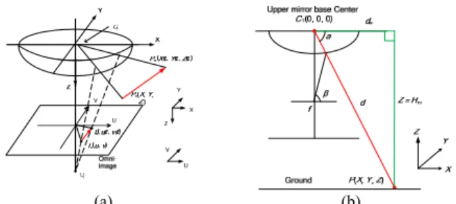
Specifically, each space point P is imaged by the two cameras in each omni-imaging device of the proposed system, resulting in two corresponding image points with coordinates (u1, v1) and (u2, v2) in the two omni- images, respectively. Using these coordinates, we look up a pano-mapping table [8] to find two corresponding elevation angles α1 and α2 with respect to the two mirror base centers C1 and C2 of the cameras, respectively, as illustrated in Fig. 2(a). To find the 3D coordinates (X, Y, Z) of P in the upper camera coordinate system (CCS), as shown in Fig. 2(b), we compute first the distance d between P and the upper mirror base center C1 according to the triangulation principle illustrated in Fig. 2(a) to get:
2 1
sin(90 ) sin( )
d b
α = α α2
+ −
D (1)
where the parameter b is the baseline length of the imaging device. Eq. (1) may be reduced to be:
2
1 2 1
cos ,
sin cos cos sin
d α b
α α α α2
= ×
× − ×
which is equivalent to:
1 1
1 .
cos tan tan
d b
α α α2
= ×
−
As a result, the horizontal distance dw and the vertical distance Z may be computed by:
1
1 2
cos tan tan dw d α b
α α
= =
− ,
1 1
1 2
sin tan
tan tan
Z d α b α
α α
= =
− . (2)
1 1 1 1
2 2 2 2
1 1 1 1
cos u sin v
u v u v
θ= − = −
+ + . (3)
Finally, we can calculate X and Y by the distance dw and the azimuth angle θ as follows:
1 2
cos cos
tan tan
X dw θ b θ
α α
= × =
− ,
1 2
sin sin
tan tan
Y dw θ b θ
α α
= × =
− . (4)
(a) (b) Fig. 2: Computing 3D data of space point using a 2-camera
omni-imaging device. (a) Light rays of a space point P projected into two cameras. (b) A triangle in (a).
3. CAR-DRIVING ASSISTANCE BY SURROUNDING ENVIRONMENT IMAGES While driving the video surveillance vehicle, we want to monitor the surrounding environment continuously in realtime for driving assistance. Owing to the wide FOV of the omni-camera and the positions of the pair of 2-camera omni-imaging devices affixed on the vehicle roof, the monitoring range of the camera system covers the entire car surround. Besides, the omni-images acquired with the omni-camera system may be used for producing multi-view images and computing the 3D information of the surrounding objects. In this study, we develop two environment monitoring applications using the camera system. One is to provide the driver a perspective-view image corresponding to the moving direction of the video surveillance vehicle, which is useful for inspection of the possible bind spots around the surveillance vehicle in order to avoid car accidents during driving. Another application is to use the proposed system as a driving recorder which records the surrounding environment images continuously during driving as a driving history, allowing the user to inspect, from any selected view direction, a sequence of perspective-view images of the vehicle surround, which are constructed in an off-line fashion from the acquired omni-image sequence.
3.1 Estimation of Optical Flows and Transformation
of Motion Vectors X1 dw cos ;1 Y1 dw sin ;1 Z1 H .m We detect motion vectors of ground points in the
consecutive omni-images by optical flow analysis using the method proposed by Lucas-Kanade [14] which analyzes optical flows of small image regions by assuming that the displacements of the image content within a small neighborhood of a point are small and approximately constant. Next, we compute the direction angle of the resulting motion vectors by transforming the vectors from the omni-image plane into the world coordinate system (WCS), as illustrated in Fig. 3(a).
The configuration of such a transformation of the motion vector of a space point on the ground is shown in Fig. 3(b). We divide the transformation process into three steps as described in the following algorithm.
(a) (b) Fig. 3: Transforming a motion vector into world coordinate
system. (a) Camera system and motion vector. (b) Ligh ray of a ground point P projected on a mirror and into a camera.
Algorithm 1: transformation of a motion vector.
Input: the beginning point P1 with coordinates (u1, v1) in an image frame It and the ending point P2 with coordinates (u2, v2) in the next frame It+1, both of the motion vector Vi of a ground point P, and the pano-mapping table T of the camera.
Output: the directional angle θi of Vi in the WCS.
Steps.
1. Compute the elevation-azimuth angle pairs (α1, θ1) and (α2, θ2) of the beginning and ending points P1
and P2, respectively, in the image coordinate system (ICS) in the following way.
1.1 Compute the azimuth angle θ1 of image point P1
with coordinates (u1, v1) by r1 = (u12 + v12)–1/2 and q1 = sin–1(v1/r1) or cos–1(u1/r1).
1.2 Using (u1, v1) to look up the pano-mapping table T to obtain the elevation angle α1 of P1.
1.3 Do similarly to obtain the elevation-azimuth angle pair (α2, θ2) for image point P2.
2. Transform the image coordinate (u1, v1) of point P1
in image It to world coordinates (X, Y, Z) of point P in the following way.
2.1 Compute the horizontal distance dw between P and the center C1 of the mirror base by dw =
Hm×cot(α1) where the distance between the center C1 and the ground is known to be Hm. 2.2 Compute as follows the world coordinates (X1,
Y1, Z1) of point P1 according to the property of rotational invariance of omni-imaging:
θ θ
× = × =
=
2.3 Do similarly to compute (X2, Y2, Z2) for point P2. 3. Compute the directional angle θi of motion vector Vi
with respect to the X-axis in the WCS by
1 2 1 1 2 1
2 2 2 2
2 1 2 1 2 1 2 1
sin or cos .
( ) ( ) ( ) ( )
i
Y Y X X
Y Y X X Y Y X X
θ = −⎛⎜ − ⎞⎟ −⎛⎜ − ⎞⎟
⎜ − + − ⎟ ⎜ − + − ⎟
⎝ ⎠ ⎝ ⎠
By Algorithm 1, we can transform all the motion vectors produced by optical flow analysis into the WCS and get the directional angles of all the motion vectors for use in analyzing the moving direction of the video surveillance vehicle, as described next.
3.2 Computation of Vehicle Moving Direction After all the outlier and noise motion vectors with too short or too long lengths are eliminated, we compute the mean of the remaining motion vectors and use it to decide the moving direction of the surveillance vehicle.
We do this by classifying the mean value, which is an angle, into three categories, moving forward, turn to the left, and turn to the right, using three angle ranges as listed in Table 1, which are determined by experiments.
Table 1: Ranges for classifying mean of motion vectors into three vehicle moving directions.
State Degree Moving forward 261°~ 279°
Turn to the left 180°~260°
Turn to the right 280°~ 360°
The above rule for deciding the vehicle moving direction is designed for analyzing a single image frame.
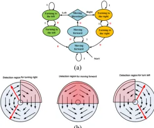
When the vehicle is moving with continuous image frames being acquired for analysis, we use the concept of finite automata (FA) to determine the vehicle moving direction in a more refined way based on the criterion of giving a second chance to the current state before it is changed. The detail of the proposed FA is shown in Fig.
4(a) where if the moving direction analysis result for the next cycle is identical to that of the current cycle, the input to the FA is taken to be “1”; else, to be “0.” Note that we take the current state in the FA as the moving direction of the surveillance vehicle in the current cycle.
On the other hand, it is observed that for different cases of vehicle moving directions (left, forward, and right), the computed motion vectors show different patterns at different regions in the omni-image.
Therefore, it is erroneous to analyze the motion vectors in an unchanged detection region in the omni-image all the time. To solve this problem, we select appropriate detection regions for the three vehicle moving direction cases, respectively, and change the detection region dynamically in accordance with the previous moving direction decision result, as illustrated in Fig. 4(b).
3.3 Generation of Perspective-view Image
After deciding the moving direction of the vehicle, we use the current omni-image frame Io to construct a perspective-view image Ip of the scene in that direction in realtime for the driver to inspect to avoid collisions
with approaching vehicles and pedestrians. The construction is based on the use of the pano-mapping table [8] again. The major steps include: (1) map each pixel p in IP with coordinates (k, l) to a pair of elevation and azimuth angles, (α, θ), in the pano-mapping table according to the geometry of the desired perspective transformation; (2) find the image coordinates (u, v) in the table corresponding to (α, θ); and (3) fill the value of pixel p in IP with that of the pixel at coordinates (u, v) in Io. The detail of mapping (k, l) to (α, θ) in Step (1) is described as follows, where it is assumed that Ip is at a distance D to the mirror base center Om and has Mp×Np pixels, and that Ip is the image of a planar rectangular W×H region AP perpendicular to the floor, as illustrated by Fig. 5.
(a)
(b)
Fig. 4: Decision of vehicle moving direction. (a) Finite automaton for deciding vehicle moving direction. (b) Detection regions for 3 cases of vehicle moving directions.
(a) (b) Fig. 5: Generation of perspective-view image. (a) Top view.
(b) A detal.
A. Computing the azimuth angle θ ⎯
The angle φ spanned by the width W of Ip as shown in Fig. 5(a) may be derived by the law of cosines to satisfy the equality of W2 = D2 + D2 − 2×D×D×cosφ so that φ may be computed to be φ = cos−1[1 − W2/(2D2)]. Also, we have β = (π − φ)/2. Let Pij denote the intersection point of the light ray RP projected onto the image point p on the planar region AP. Then, we may compute the distance d between Pij and the border point Pr shown in Fig. 5(b) by linear proportionality to be d = k×W/MP
because region AP has a width of W, image Ip has a width of Mp, and pixel p has the horizontal coordinate k.
Furthermore, the distance L between Pij and the mirror base center Om shown in Fig. 5(b) satisfies the equality of L2 = D2 + d2 − 2×d×D×cosβ. And the distance h from Pij to the line segment OmPr may be computed to be h = d×sinβ. Finally, the azimuth angle θ of Pij with respect to OmPr satisfies the equation sinθ
= h/L which, by the equalities derived above, leads to:
θ = sin−1(h/L) = 1 2 2 sin
2 cos
d
D d d D
sin β .
β
− ⎛⎜⎜⎝ + − × × ×× ⎞⎟⎟⎠ (5) B. Computing the elevation angle α ⎯
As illustrated in Fig. 6, the height of region AP is H and image Ip is divided into Np intervals vertically. So, by linear proportionality, the height of Pij is just Hp = (l×H)/Np where l is the vertical coordinate of pixel p.
Finally, by trigonometry the elevation angle α may be derived to be α = tan−1(Hp/L). Note that in the above derivations, the start direction (specified by the line segment OmPr) of the angle φ spanned by the width W of Ip, as shown in Fig. 6, coincides with the horizontal direction (i.e., with the direction of 0o). The azimuth angle θ is measured from this direction.
ρe
N Om
D H
ρs
ρq Hp
NQ l ρe
N Om
D H
ρs
ρq Hp
NQ l
Fig. 6: Lateral view of perspective-view image.
3.4 Construction of Perspective-Mapping Tables In the previous process of generating perspective- view images, we have the mappings (k, l) → (α, θ) → (u, v). This means that we can generate a new type of table, called perspective-mapping table, to record the mapping (k, l) → (u, v) directly (skipping (α, θ)) to accelerate the speed of generating the perspective-view image. Furthermore, for monitoring of the vehicle surround, generation of perspective-view images of the six directions of 0o, 60o, …, 300o around the vehicle are sufficient. Therefore, we create six perspective-mapping tables of these directions for use in this study. Some experimental results are shown in Fig. 7.
4. MONITORING OF A NEARBY STATIC CAR FROM A STATIC VEHICLE The proposed method for monitoring a nearby static car when the video surveillance vehicle is also in a static state include the major steps of (1) nearby car detection; (2) car window side extraction; (3) car distance estimation; and (4) surround map generation.
Om
Pij
β Pr D
θ L h d( P
W φ β
Om D
θ pi
The final result is a top-view surround map showing the graphic shapes of the detected nearby car and the surveillance vehicle located in relative postures (positions and orientations).
(a) (b)
(c) (d)
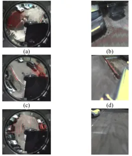
(e) (f) Fig. 7: Car direction detection and generated images. (a)
Turning to left. (c) Turning to right. (e) Moving forward.
(b), (d), and (f) Corresponding perspective-view images.
4.1 Nearby Vehicle Detection
To detect the existence of a nearby static car, we have to segment out the objects existing in an omni-image first. We assume the environment to be a drive way or a parking lot where the road surface is roughly uniform in gray color. To conduct object segmentation, first we
“learn” the gray value of the road surface from the two omni-images acquired with the two cameras in each omni-imaging device. Each original omni-image Io then is transformed into a grayscale one Ig. A region of the ground is manually selected next, and the mean gray value gm of the region is computed. A difference image f then is generated by subtracting gm from the gray value of each pixel in Ig. Possible car regions are segmented out from Ig by thresholding the difference image f into a binary image B by moment-preserving thresholding proposed by Tsai [21]. Noise components are removed from B finally using a region growing scheme. A result of this process is shown in Fig. 8.
(a) (b) (c) Fig. 8: Nearby car detection result. (a) Original image. (b)
Binary image with ground portion in (a) removed before noise elimination. (b) Image after noise elimination.
4.2 Car Window Side Extraction
We try to detect the edge points of the car window
from the omni-image, as illustrated in Fig. 9, by scanning the points on a radial line, starting from the image center to the image boundary. In this process, it is necessary to make sure that the points extracted are not just noise points. For this, only a sufficiently large number of consecutive points on the radial line are considered as a window edge. The detail is described as follows.
Fig. 9: Detecting window edge points in binary image.
Algorithm 2: detecting car window edge points.
Input: a binary image B with detected car body pixels labeled by 1 and others labeled by 0.
Output: car window edge points.
Steps.
1. (Collecting car door pixels) Scan the car body pixels labeled by 1 sequentially on each unscanned radial line, starting from the image center, and perform the following two steps.
1.1 Collect pixels sufficiently close to each other (apart for a distance smaller than a threshold TH1).
1.2 If the number of points so collected is large enough (larger than a threshold TH2), then go to Step 2; else, abandon the collected pixels and go to Step 1 if there is any unscanned radial line or exit if none.
2. (Collecting car window pixels) Continue scanning on the radial line to collect non-car body pixels labeled by 0 sequentially, and perform the following two steps.
2.1 Collect pixels sufficiently close to each other (apart for a distance smaller than TH1).
2.2 If the number of points so collected is large enough (larger than TH2), then go to Step 3; else, abandon the collected pixels and go to Step 1 if there is any unscanned radial line or exit if none.
3. (Marking a car window edge pixel) Mark the beginning pixel of the collected ones in Step 2 as a car window edge pixel and go to Step 1 if there is any unscanned radial line or exit if none.
Algorithm 2 above is performed for each of the two omni-images acquired by each omni-imaging device used in this study. However, we cannot confirm that all the collected window edge points by Algorithm 2 are useful. We have to find out the real point pairs of the window edges collected from the two omni-images. The detail to do so is described in the following algorithm.
Algorithm 3: collecting useful pairs of corresponding points of the car window edge.
Input: two sets Bupper and Blower of candidate window edge pixels collected by Algorithm 2 from the omni-images acquired respectively by a pair of upper and lower cameras.
Output: a set Bcar of real consecutive pixel pairs of the car window edge.
Steps.
1. For each unscanned azimuth angle θ, starting from 0o, check if there exist two pixels in the sets Bupper
and Blower, respectively, which have the same azimuth angle θ; if so, mark them as a candidate pair.
2. For every two consecutive candidate pairs of Bupper
(or Blower), if the difference between the radius distances of the two pairs is smaller than a threshold value TH3 and the difference between the azimuth angles of the two pairs is smaller than another threshold value TH4, then mark the two pairs as useful pairs.
3. Check if the number of useful pairs in Bupper (or Blower) is larger than a third threshold value TH5, then mark the pixels in all the useful pairs as coming from the car window edge and put them into the desired set Bcar for computing the 3D data of the car window and exit; else, abandon the collected useful pairs so far and go to Step 2 if there are more than two unchecked candidate pairs; or exit, else.
A result of the above algorithm is shown in Fig. 10.
(a) (b) Figure 10: Car window side extraction. (a) Input image.
(b) Result (red points) of extraction superimposed on (a).
4.3 Car Distance Estimation
Each useful pair in Bcar has two corresponding image points, one from the upper omni-image and the other from the lower omni-image. Their coordinates therefore can be used to compute 3D data of the corresponding space point Pi according to the process described in Sec.
2.2 (see Eqs. (2) and (4)), with the height and distance of the space point with respect to the mirror base center being specified as Z and dw, respectively, there. Here, let the height and the distance of the space point corresponding to each useful pair collected in Bcar be denoted as Hi and Di, respectively, and let the total number of useful pairs in Bcar be denoted as n. Then, we compute the mean values of all Hi and Di, respectively, and take them to represent the height Hcar and distance Dcar of the detected car. Also, we take the azimuth angle θcar (mentioned in Step 1 of Algorithm 3) of the middle of all the useful pairs in Bcar to be the azimuth angle θcar
of the detected car. These data are used for generating a surround map, as described next.
4.4 Generation of a Top-view Surround Map
With the horizontal distance Dcar and the azimuth angle θcar, the relative position of the detected car can be described by the coordinates (ucar, vcar) in a top-view 2D coordinate system created as the desired surround map, where (ucar, vcar) are computed as:
ucar = (Dcar×cosθcar)/ratio; vcar = (Dcar×sinθcar)/ratio with ratio being a factor to scale the real distance Dcar in the WCS down into the top-view 2D coordinate system.
To generate the surround map, first we initialize a gray background image I like that of an asphalt road.
Then, we paste a graphic shape of the surveillance vehicle at the center of image I. Finally, we select the front-right corner of the surveillance vehicle shape as the origin (0, 0) of the mentioned top-view 2D coordinate system and paste a graphic shape of the detected nearby car on I at coordinates (ucar, vcar) computed above. A result is shown in Fig. 11.
θcar
Fig. 11: A surround map from the top view.
5. MONITORING OF A NEARBY STATIC OR MOVING CAR FROM A MOVING
SURVEILLANCE VEHICLE
When the surveillance vehicle is moving, the method of the last section is not applicable for nearby car detection. Instead, optical flow analysis is used in this study, based on the observation: if the concerned object is higher than the ground, its motion appearing in the image will produce motion vectors with larger lengths.
This property may be used to segment the car from the background. Four major steps are performed for monitoring a static or moving nearby car when the surveillance vehicle is moving: (1) motion vector computation; (2) nearby car detection; (3) car distance estimation; and (4) surround map generation.
5.1 Nearby Car Detection by Motion Vectors
First, we divide the omni-image into blocks and use the center points of the blocks to compute the motion vectors by optical flow analysis. The motion vectors then are transformed from the ICS into the WCS by Algorithm 1. Next, we make use of the above- mentioned property to extract roughly the motion vectors of a nearby car in the following way: (1) compute the average L and the standard deviation S of the lengths of all the motion vectors; (2) classify each motion vector Vi as from the ground if Vi < L – S; as from the car if Vi > L + S; and as ambiguous, else; (3)
take as the desired rough car region all those blocks with corresponding motion vectors classified as from the car. A result of this process is shown in Fig. 12(a).
(a) (b) (c) Fig. 12: Near by car detection with surveillance vehicle moving. (a) Rough car detection result. (b) Result of k- mean clustering and region growing. (c) Binary image corresponding to (b).
Furthermore, it is desired to detect more precisely the car body pixels from the rough car region. For this, we use the k-means algorithm with k = 3, meaning the three classes of car body, car window, and noise. The input feature is pixel color. Having the result of the algorithm, we apply region growing to obtain the car body region, starting from the largest cluster with its center’s color different from that of the ground, gm, which was learned in advance (see Sec. 4.1). During the process, pixels with colors close to gm are also ignored, and only those with colors close to that of the cluster center are grown.
A result of this process is shown in Figs. 12(b) and (c).
5.2 Car Distance Estimation and Surround Map Generation
To estimate the location of a nearby car detected as above, the approach we adopt is to match the detected car region by a car mask to estimate the car position, which includes two stages: (1) generation of car masks by transforming a pre-selected car model of the shape of a rectangular parallelepiped from the WCS into the ICS; and (2) computation of the nearby car location by a template matching scheme.
A. Generation of car masks
By imagining a rectangular-parallelepiped-shaped car model on the X-Y plane as shown in Fig. 13(a), it is desired to transform the model onto the image plane as shown in Fig. 13(b) to generate a series of car masks, which then are used to match the detected car shape in order to locate the car. To generate a car mask, under the assumption that the mirror base center Om of the omni-camera is located at coordinates (X0, Y0, Z0) in the WCS, for each space point P with world coordinates (X, Y, Z) of the car model, we compute first the distance between P and Om as d = [(Xi – X0)2 + (Yi – Y0)2]–1/2 Then, we can compute, according to the discussions of Sec. 2.2, the elevation-azimuth angle pair to be
θ = cos–1[(Xi – X0)/d] = sin–1[(Yi – Y0)/d], ρ = (π/2) − tan−1[(Zi − Z0)/d].
Then, we look up the pano-mapping table of the camera to find the corresponding image coordinates (u, v) of a pixel of the desired car mask.
B. Computing the car location by template matching
To locate the detected car in the omni-image, then we use template matching to superimpose each of the generated car mask on the detected car region as shown in Fig. 13 using the previously-computed coordinates of the mask points. Then, we check the overlapping ratio of each matching, and find out the optimal mask M which yields the largest ratio. The center of M is finally computed and taken to be the position of the detected car. A graphic shape for the detected nearby car then is drawn on the desired surround map accordingly in a way of scaling down like that described in Sec. 4.4. A result of this process is shown in Fig. 14.
(a) (b) (c) Fig. 13: Car location by matching car mask and car region. (a)
Car model in WCS. (b) The mask image. (c) Result of matching detected car by a mask.
(a) (b) Fig. 14: Detecting static nearby car from moving vehicle. (a)
Original image. (b) Generated surround map (direction of car is 180o reversed when compared with real situation in (a)).
6. EXPERIMENTAL RESULTS
Many experiments were conducted on an open space area, including a parking lot and a spacious around- campus road with asphalt surfaces. Some experimental results have been shown previously. One more result of static nearby car detection from a static vehicle is shown in Fig. 15. Another result of nearby car detection from a moving vehicle is shown in Fig. 16. Though it is worth to conduct accuracy analysis about various detection results, all the results indicate that the proposed system is practical for real applications.
7. CONCLUSIONS
In this study, a video surveillance system utilizing a pair of 2-camera omni-imaging devices equipped on the roof of a video surveillance vehicle to monitor the surrounding environment has been proposed.
Specifically, a technique for detecting vehicle driving directions and generating corresponding perspective- view images for car-driving assistance has been proposed. Also have been proposed are techniques for detecting a nearby static car from a static surveillance
vehicle as well as for detecting a nearby static or moving car from a moving vehicle. Corresponding top- view surround maps can also be generated to help the driver to inspect the vehicle surround conditions. The experimental results show the feasibility of the proposed system and techniques. Future studies may be directed to detecting multiple nearby cars or persons from a moving surveillance vehicle, and improving the computation speed of the system.
(a) (b) (c) Fig. 15: Result of detecting a nearby static car from a static
vehicle. (a) & (b) Two original image frames. (c) Generated surround map (car direction is 180o reversed).
(a) (b) (c)
(d) (e) (f) Fig. 16: Result of nearby static car detection from a moving
vehicle. (a)-(c) Original image frames. (d)-(f) Respective generated surround maps (car direction is 180o reversed).
REFERENCES
[1] C. Micheloni, G.L. Foresti, C. Piciarelli and L. Cinque,
“An autonomous vehicle for video surveillance of indoor environments,” IEEE Trans. on Vehicular Technology, vol.
56, no. 2, March 2007.
[2] G.L. Foresti, C. Micheloni and L. Snidaro, “Event classification for automatic visual-based surveillance of parking lots,” Proc. 17th Int’l Conf. on Pattern Recognition, vol. 3, pp. 314–317, 2004.
[3] M. Bramberger, R. P. Pflugfelder, A. Maier, B. Rinner, B.
Strobl and H. Schwabach, “A smart camera for traffic surveillance,” Proc. 1st Workshop on Intelligent Solutions in Embedded Systems, pp. 153–164, Vienna, Austria, 2003.
[4] Y. Onoe, N. Yokoya, K Yamazawa, and H. Takemura,
“Visual surveillance and monitoring system using an omnidirectional video camera,” Proc. 1998 Int’l Conf. on Pattern Recog, vol. 1, pp. 588–592, Brisbane, Australia, Aug. 16-20, 1998.
[5] T. Mituyosi, Y. Yagi, and M. Yachida, “Real-time human feature acquisition and human tracking by omnidirectional image sensor,” Proc. IEEE Int’l Conf. on Multisensor Fusion & Integration for Intelligent Systems, pp. 258-263, Tokyo, Japan, July-Aug. 2003.
[6] L. He, C. Luo, F. Zhu, Y. Hao, J. Ou and J. Zhou, “Depth map regeneration via improved graph cuts using a novel
omnidirectional stereo sensor,”Proc. 11th IEEE Int’l Conf.
on Computer Vision (ICCV2007), pp. 1-8, Oct. 14-21, Rio de Janeiro, Brazil, 2007.
[7] H. Koyasu, J. Miura, and Y. Shirai, “Realtime omnidirectional stereo for obstacle detection and tracking in dynamic environments,” Proc. 2001 IEEE/RSJ Int’l Conf. on Intelligent Robots and Systems, pp. 31-36, Maui, Hawaii, USA, Oct./Nov, 2001.
[8] S. W. Jeng and W. H. Tsai, “Using pano-mapping tables for unwarping of omni-images into panoramic and perspective-view images,” Journal of IET Image Processing, Vol. 1, No. 2, pp. 149-155, June 2007.
[9] T. Ehlgen and T. Pajdla, “Maneuvering aid for large vehicle using omnidirectional cameras,” IEEE Workshop on Applications of Computer Vision, pp. 17–17, Austin, Texas, US, Feb. 2007.
[10] T. Gandhi and M.M. Trivedi, “Motion analysis for event detection and tracking with a mobile omni-directional camera,” ACM Multimedia Systems Journal, Special Issue on Video Surveillance, vol. 10, no. 2, pp. 131–143, 2004.
[11] N. Murakami, A. Ito, Jeffrey D. Will , Michael Steffen, K. Inoue, K. Kita, S. Miyaura, “Development of a teleoperation system for agricultural vehicles,”
Computers and Electronics in Agriculture, vol. 63, pp.
81-88, Aug. 2008.
[12] R. Aufrère, J. Gowdy, C. Mertz, C. Thorpe, C.C. and T.Y. Wang, “Perception for collision avoidance and autonomous driving,” Mechatronics, Vol. 13, pp. 1149- 1163, 2003.
[13] C. Hughes, M. Glavin, E. Jones and P. Denny, “Wide- angle camera technology for automotive applications: a review,” IEEE Trans. on Intelligent Transportation Systems, vol. 3, no. 1, pp. 19–31, 2009.
[14] B. D. Lucas and T. Kanade, “An iterative image registration technique with an application to stereo vision,” Proc. 7th Int’l Joint Conf. on Artificial Intelligence, Vancouver, Canada, pp. 674–679, 1981.
[15] J. Kim and Y. Suga, “An omnidirectional vision-based moving obstacle in mobile robot,” Int’l J. of Control, Automation, & Systems, vol. 5, no. 6, pp. 663-673, Dec.
2007.
[16] S. Gupte, O. Masoud, R.F. K. Martin, and N.P.
Papanikolopoulos, “Detection and classification of vehicles,” IEEE Trans. on Intelligent Transportation Systems, vol. 3, no. 1, Mar. 2002.
[17] R. Cucchiara, M. Piccardi, and P. Mello, “Image analysis and rule-based reasoning for a traffic monitoring system,” IEEE Trans. on Intelligent Transportation Systems, vol. 1, no. 2, June 2000.
[18] L. W. Tsai, J. W. Hsieh and K. C. Fan, “Vehicle detection using normalized color and edge map,” IEEE Trans. on Image Processing, vol. 16, no. 3, Mar. 2007.
[19] P. H. Yuan, K. F. Yang and W. H. Tsai, “Security monitoring around a video surveillance car with a pair of two-camera omni-directional imaging devices,” Proc.
2010 Workshop on Image Processing, Computer Graphics, & Multimedia Technologies, Int’l Computer Symp., pp. 325-330, Tainan, Taiwan, Dec. 2010.
[20] C. J. Wu, “New localization and image adjustment techniques using omni-cameras for autonomous vehicle applications,” Ph. D. Dissertation, Institute of Computer Science and Engineering, National Chiao Tung University, Hsinchu, Taiwan, July 2009.
[21] W. H. Tsai, “Moment-preserving thresholding: a new approach,” Computer Vision, Graphics, and Image Processing, vol. 29, no. 3, pp. 377-393, 1985.