國立臺灣大學電機資訊學院資訊工程學系 碩士論文
Department of Computer Science and Information Engineering College of Electrical Engineering and Computer Science
National Taiwan University Master Thesis
具自動設定之駕駛輔助系統在智慧型手機上的應用 A Calibration Free Driver Assistance System on Mobile Phone
許焙凱 Hsu Pei-Kai
指導教授:莊永裕 博士
中華民國 99 年 1 月
Jan, 2010
摘要
行車駕駛輔助系統是保護駕駛人及用路人安全很重要的設備之一,但是這種行車駕駛輔 助系統通常由雷達或影像辨識技術達成,雷達系統因為配備昂貴通常是在高階的房車才會裝 有這種系統,而影像辨識系統以目前的研究技術都要搭配相當高階的電腦系統如 Intel Penten-4 3.0G CPU + 1G Ram 才能達到與雷達系統相當的水平。 我們認為如果要在車上裝 一台這麼高階的電腦系統才能成為行車駕駛輔助系統勢必是沒有使用者能接受,所以本論文 的研究著重在尋求一套好的演算法能夠在準確度與裝置效能上達到一個平衡點。
現今,智慧型手機越來越普及化,RISC CPU 運算能力已經能達到 500MHz 以上,加上它 目前都具有 Camera 及 GPS 功能,體積上也相當適合裝置在車上,而且 Microsoft 也從 Windows Mobile 5.0 以後訂出了透過 Direct Show 控制 Camera 及 GPS 的標準界面,所以我 們選擇在智慧型手機上開發一套行車駕駛輔助系統讓擁有智慧型手機的駕駛人除了把智慧型 手機拿來做導航外能多出行車駕駛輔助系統功能。
傳統的影像辨識技術除了需要運算能力很高階的電腦外,另一個問題就是架設上非常繁 瑣,通常需要知道相機鏡頭的參數及架設位置,一般使用者很難自行去架設這樣的一個系統,
所以我們的系統在設計時加入了這個考量,特別搭配 GPS 設計出不需要知道相機鏡頭參數及 架設位置就能自動校正系統並且辨識出可能的車距。
我們的系統使用 HTC Diamond 1 (P3700)這款智慧型手機做實驗,其具備 QUALCOMM 7201A 的 RISC CPU,CPU 速度為 528MHz 及 192MB RAM,是目前最普遍的智慧型手機架構,實驗證實 我們的演算法能在這樣的系統上在 100 毫秒內處裡一個 frame,也就是說我們能提前 100 毫 秒就通知駕駛人可能發生的危險,保護其生命安全。
關鍵字: 行車輔助系統、智慧型手機、電腦視覺、Windows Mobile、車道偵測、GPS、相機
Abstract
A driver assistance system is an important device to keep the driver and passerby safe. This kind of device consists of radar system or computer vision in general. The radar system just sets in high-end cars and is very expensive. The computer vision system needs powerful computer with Penten-4 3.0G CPU and 1 gigabytes memory for qualifying with radar system. Most users need a useful driver system but might have difficulties to set this kind of computer devices. In this thesis, we have tried to develop an algorithm which has the competence in balancing the performance and the accuracy of this kind of system.
The smart phone becoming increasingly popular now, it has RSIC CPU which fast than 500 MHz and has camera and GPS system. The size of smart phone is also suite for setting on car.
Microsoft had supported camera controlling by “Direct Show” and GPS APIs after Windows Mobile 5.0. Therefore, we chosen smart phone to be our target development device. We wish to make the smart phone not only has navigation function but also driver assistance system.
The traditional computer vision system needs a powerful computer and complexity setup routine. Usually, users need to provide the focus length of camera and setting position. It is hard for users to set up this kind of system by themselves. By the way, we collocate with GPS to design an auto calibration system to avoid this complex set up routine.
We chose HTC Diamond 1 (P3700) to be our experiment device. It has QUALCOMM 7201A RISC CPU which has 528MHz CPU speed and 192 mega bytes ram. This is the most popular smart phone architecture recently. We verified that we can make a decision in 100 milliseconds by our algorithm with this device. In other words, we can alert the driver an emerging danger 100 milliseconds n advance and keep them safe.
Key words: Driver Assistance System, Smart Phone, Computer Vision, Windows Mobile, Lane Detection, GPS, Camera
Table of Contains
摘要………..………..….i
Abstract……….……….ii
Chapter 1 Introduction ……….1
1.1 Motivation……..………..……….1
1.2 Related Work………….……….……….2
1.3 Objective………..……….3
1.4 System Overview……….3
1.5 Organization of this thesis………..……….5
Chapter 2 Road Cropping………..…….6
2.1 HSV Color Model………..……….6
2.2 Lane Filter..……….9
2.3 Cache Enhance Lane Filter Coding………....….9
2.4 Lane Probed Algorithm……….……….11
2.5 Road Area Conjecture……….14
Chapter 3 Accurate Lane Detection………..……….17
3.1 Image Normalization………..……….17
3.2 Lane and Vehicle Detection………..……….18
3.3 Extract Lane……….21
3.4 Lane Model………..……….21
3.5 Slope Histogram………..……….23
3.6 Lane Voting……….……….23
Chapter 4 Vehicle Detection……….27
4.1 Detect Vehicle by the Shadow……….27
4.2 C-means……….27
Chapter 5 Auto Calibration………..……….29
5.1 GPS……….……….29
5.2 Auto Calibration……….29
Chapter 6 Distance Measurement………….……….32
Chapter 7 Experiment………….……...……….33
7.1 Hardware Environment Description……….33
7.2 Software Environment Description………..……….34
7.3 Get Image by Direct Show……….……….……….34
7.4 Experiment Result……….35
Chapter 8 Conclusions and Future Works……..…..………37
Reference……….………..……….38
List of Figure
Figure 1.1: Flowchart of the system………4
Figure 2.1: A High Way Image………..………..…6
Figure 2.2: HSV color wheel………7
Figure 2.3: HSV cone.………….……….8
Figure 2.4: (a) Original Image. (b) The image applied the lane filter. (c) The image processed withlane probe algorithm………14
Figure 2.5: (a) Lane pattern. (b) Others……….14
Figure 2.6: (a) Overlap image. (b). Horizontal histogram………….……….15
Figure 3.1: (a) Original image. (b) Normalization image………18
Figure 3.2: (a) Original image. (b) Normalization image. (c) Separated lane image from normalization image. (d) Separated vehicle image from normalization image...20
Figure 3.3: (a) Lane marker image. (b) Linear fitting result…….……….22
Figure 3.4: The flow chart of pre-process lane image for lane voting……..……..24
Figure 3.5: (a) Matching left lane. (b) Matching right lane……….25
Figure 3.6: Lane voting result………..……….………. 26
Figure 4.1: Vehicle searched area…………..………..27
Figure 4.2: (a) Real image. (b) Vehicle markers image……….28
Figure 5.1: The sketch map of calibration parameter………....30
Figure 5.2: Perspective projection of ground plane and the relationship of parabolic curve……….30
Figure 6.1: The example of front car distance measuring result………32
Figure 7.1: HTC Touch Diamond P3702……….33 Figure 7.2: The flow chart of our Direct Show filters link.………..35 Figure 7.3: Front vehicle tracking and distance measure.
(a) 120 meters away from the vehicle in front.
(b) 132 meters away from the vehicle in front.
(c) 117 meters away from the vehicle in front.
(d) 106 meters away from the vehicle in front…….……….……..36
List of Tables
Table 1.1: Related factors for 2007 high way traffic accident in Taiwan………..2
Table 7.1: Hardware system information…..………..………..34
Table 7.2: Software system information………...34
Chapter 1
Introduction
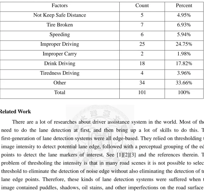
1.1 MotivationAccording to the statistics of National Police Agency, there were about 24.75% of vehicle drivers died in the improper driving and 4.95% died in not keeping safety distance on the highway traffic accidents in 2007. The related factors are listed in Table 1.1. From these factors we can see that the improper driving is the major traffic accident. There are many kinds of driver assistance systems such as the millimeter wave radar, the laser radar and the ultrasonic radar system. Although they have high accuracy and performance advantages, but it is an expensive device and just the high-end cars can be provided with this kind of system.
Therefore, many people try to do some researches in order to use CCD camera to replace its function. However, We do not think this application is a good solution. They can use a cheap CCD camera to replace radar device, but the powerful calculation system and setup step is not good solution for a driver. Users need to setup a powerful PC with a CPU faster than Intel Pentium IV 2.4GHz and also a 256MB Ram with accurate setting steps for the CCD. It is not a good succedaneum for driver. By the way, we think that the smart phone is a good device for this application because it has CMOS camera and portable advantages. Users can set it up free, but the challenge is its computing power. All smart-phone devices just provide RISC CPU and small RAM. So, we need to design an algorithm that is suitable to this system and to get a balance in the performance and accuracy.
Table 1.1 Related factors for 2007 high way traffic accident in Taiwan
Factors Count Percent
Not Keep Safe Distance 5 4.95%
Tire Broken 7 6.93%
Speeding 6 5.94%
Improper Driving 25 24.75%
Improper Carry 2 1.98%
Drink Driving 18 17.82%
Tiredness Driving 4 3.96%
Other 34 33.66%
Total 101 100%
1.2 Related Work
There are a lot of researches about driver assistance system in the world. Most of them need to do the lane detection at first, and then bring up a lot of skills to do this. The first-generation of lane detection systems were all edge-based. They relied on thresholding the image intensity to detect potential lane edge, followed with a perceptual grouping of the edge points to detect the lane markers of interest. See [1][2][3] and the references therein. The problem of thresholing the intensity is that in many road scenes it is not possible to select a threshold to eliminate the detection of noise edge without also eliminating the detection of true lane edge points. Therefore, these kinds of lane detection systems were suffered when the image contained puddles, shadows, oil stains, and other imperfections on the road surface or the lanes in image with low contrast, broken, occluded and totally absent.
The second generation of the systems sought to overcome these problems by directly working with the image intensity. For example, K.C. Kluge [3] used the global road shape constraints derived from an explicit model of how the features defining a road appear in the image plane. Using the simple one-dimensional edge detection will be followed by a least median squares technique to determine the curvature and orientation of the road. The D.
Pomerleau system [4] is another example of a second generation lane detection system. It is a matching technique that with adaptively adjust and aligns a template to the averaged scan line intensity profile in order to determine the lane’s curvature and lateral offsets. There are several
other such second generation systems [5]and many of these have been subjected to several hours of testing, which involved the processing of extremely large and varied data set.
The third generation of the system detects the lane directly on color image. For example Kuo-Yu Chiu [6] used to find out lane boundary by color information. This system demands low computational power and memory requirements, and is robust in the presence of noise, shadows, pavement, and obstacles such as cars, motorcycles and pedestrian conditions.
Another similar system is described in [7]. The effectiveness and reliability of these warning/control systems are contingent on the performance of the underlying lane detection algorithm.
1.3 Objective
In order to design a popular and friendly system for most people, we chose the windows mobile base smart phone as our target system. The smart phone has three import components, Camera, CPU and GPS system. The camera is used as a sensor of computer vision. The GPS is used to get speed information and help system to do the auto calibration. And the CPU is main calculator and controller. But the CPU in smart phone is not powerful as in PC. It is RISC architecture CPU and do not have floating point operation and large cache. Therefore, we cannot expect that to have the detected quality which is equal to PC like system or radar system. Our aim is to make a decision in 100 milliseconds basing on the system with 500MHz RISC CPU. HTC Diamond (P3700) was chosen to be our developed device, because it has Qualcomm 7201A 528MHz CPU, 192MB SDRAM, Camera module, GPS module and fully support Direct Show APIs which let as easily to control the camera module. The image resolution in this device is 240x320 with preview mode.
1.4 System Overview
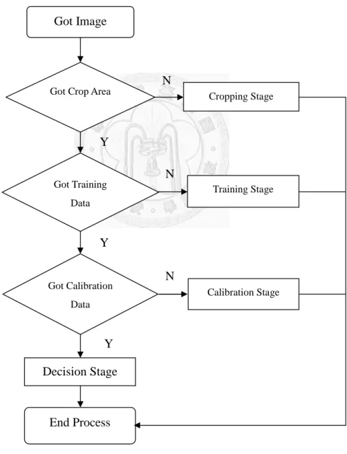
In our system, we separate four stages to start up the system, cropping, training, calibration and decision. The cropping stage is used to reduce calculation area. In this system, we just need to detect road surface. Therefore, we firstly will crop road surface area in this stage. The training stage is used to reduce calculation complexity at decision stage. Secondly,
in this stage we will use the complex lane detection algorithm to detect the real lane segment and following with some statistic about the lane attributes in these frames. Thirdly, we will use these lane attributes to do the lane detection accelerated in the decision stage. Because we do not need user to input some camera and set up coefficients, we cannot calculate the distance of the vehicle in the front from 2D image directly. The calibration stage will collect speed and time information from GPS and calculate the mapping of the front car distance in 2D image and real world system. Finally, we can use these training data to help the facile lane and vehicle detection process in decision stage. Figure 1.1 shows the flowchart.
Figure 1.1: Flowchart of the system.
Got Crop Area
Got Training Data
Got Calibration Data
Decision Stage Got Image
End Process
Cropping Stage
Training Stage
Calibration Stage
N
N
N Y
Y
Y
1.5 Organization of this thesis
The rest of this thesis is organized as follows: Chapter 2, describes how to crop a useful area for reducing computing area; Chapter 3, describes how to detect lane segment with our accurate algorithm and gets correct lane model; Chapter 4, describes how to detect the front vehicle and its position by shadow and C-means algorithm; Chapter 5, provides an algorithm about how to map the front vehicle distance from 2D image to real world 3D coordinate;
Chapter 6, describes how to use the parameters got from pre-chapter to make a decision;
Chapter 7, gives the experimental result; and Chapter 8 concludes our works and remark on some possible future works.
Chapter 2
Road Cropping
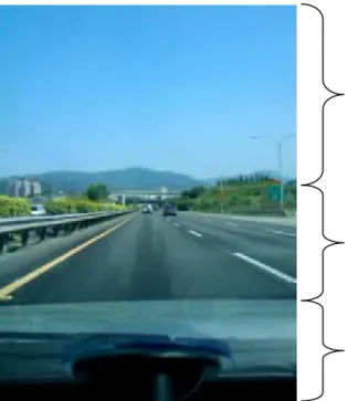
Road cropping stage is used to reduced calculate area. Base on our application, we only need to calculate road area in the image. The composition of a high way image is very complex in road area but clear in sky and cabin area such as in Figure 2.1. From Figure 2.1, we can realize that lanes are comprised of a lot of oblique line segments. So, we can use ±45° line edge filter to filter out lane segments and do a horizontal histogram to isolate road area.
Figure 2.1: A High Way Image
2.1 HSV Color Model
In our system, we use color information and line structure to do the lane and vehicle detections. The true color image is hard to do computer vision especially to the object outline and the edge analysis. In general, the gray image is good for edge detection. Therefore, we need to transform image form the true color to the gray level image. We chose HSV color space to be our process domain.
Road Area Sky Area
Cabin Area
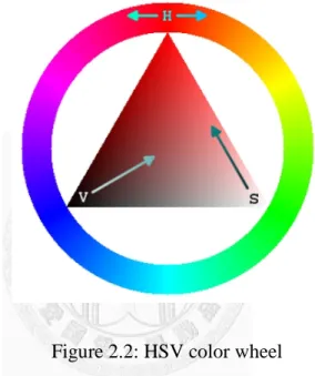
The HSV model is commonly used in the computer graphics applications. In various application contexts, a user must choose a color to be applied to a particular graphical element.
When used in this way, the HSV color wheel in Figure 2.2 is mostly used. In it, the hue is represented by a circular region; a separate triangular region may be used to represent the saturation and the value. Typically, the vertical axis of the triangle indicates saturation while the horizontal axis corresponds to value. In this way, a color can be chosen by first picking the hue from the circular region, and then selected the desired saturation and value from the triangular region.
Figure 2.2: HSV color wheel
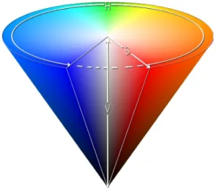
Another visualization method of the HSV model is the cone in Figure 2.3. In this representation, the hue is depicted as a three-dimensional conical formation of the color wheel.
The saturation is represented by the distance from the center of a circular cross-section of the cone, and the value is the distance from the pointed end of the cone. This method is well-suited to visualize the entire HSV color space in a single object.
Figure 2.3: HSV cone.
Here is the formula of conversion form RGB color model to HSV color model. In our application the value range of Red, Green and Blue is 0~255.
h =
⎩⎪
⎨
⎪⎧0, if max = min 60° × + 360° mod 360°, if max = r
°× °, °× °,
(2.1)
s = 0, if max = 0
= 1 − , otherwise (2.2) v = max (2.3) l r, g, b ∈ [0,255].
l h: The hue angle, where h ∈ [0,360].
l s: The saturation.
l v: The lightness.
l max: The greatest of r, g and b.
l min: The least of r, g and b.
2.2 Lane Filter
From Figure 2.1, we realized that the road area composes with the lanes, vehicle, traffic signs, plants and so on. The composition is very complex. The sky area does not have obvious line segments. And the cabin area just has some fix horizontal lines. Therefore, we will apply a lane filter to the gray scale image and do a horizontal histogram from the edge image. From the histogram, we can segment out the road area easily. From Figure 2.1, we also understood that the lane is composes with the oblique lines. The vector of lanes in the left part of image is positive and negative in the right part of image. So, we used two 3x3 matrices to filter out these line segments. Below is our filters and formula.
g(x, y) = ∑ ∑ LM(s, t)f(x + s, y + t), if x ≤ (width 2 )
∑ ∑ RM(s, t)f(x + s, y + t), if x > (width 2 ) (2.4) l LM = 1 0 0
1 0 −1 0 0 −1 l RM = −1 0 0
−1 0 1 0 0 1
g (x, y) = 255, if|g(x, y)| ≥ 80 and g(x, y) ≥ 0
128, if|g(x, y)| ≥ 80 and g(x, y) < 0 (2.5) After applying the lane filter, we can get a sketch image such as in Figure 2.4 (b). This image involves some edge which is not the lane edge. These wrong edges will cause wrong histogram result. So we need another algorithm to pick out these edges. The formula 2.5, in addition to figure out the edge, marks the lane attribute is the other important process.
2.3 Cache Enhance Lane Filter Coding
The RISC CPU always has weak cache system. The CPU on our experiment device is Qualcomm 7201A. It is ARM 11 family and just has 16K bytes I-Cache and D-Cache. Where the original data is expensive to fetch (owing to longer access time) or to do the computing, compared to the cost of reading the cache. In other words, a cache operate is used as a temporary storage area where frequently accessed data can be stored for rapid access. Once the data is stored in the cache, it can be used in the future by accessing the cached copy rather than re-fetching or re-computing the original data. Hence we should avoid the cache miss as much
current stack which should be in cache memory and do the 3x3 filter each times. After the filter process has done we can move the memory point, copy one processed line to the target image memory and just copy next new line from the memory to the memory in the cache. According to our experiment, this skill can be improved about 30% in the performance than operating the memory directly while doing the filter process. In the below is our coding sample of this cache enhancement skill on lane filter.
static unsigned char *proc_line;
static unsigned char *up_line;
static unsigned char *bt_line;
static unsigned char *cp_line;
static unsigned char *p_proc_line;
static unsigned char *p_up_line;
static unsigned char *p_bt_line;
static unsigned char *p_cp_line;
static unsigned char *p_temp;
static unsigned char linecache[960];
p_up_line = up_line = linecache;
p_proc_line = proc_line = linecache+240;
p_bt_line = bt_line = linecache+480;
p_cp_line = cp_line = linecache+720;
int addr;
int addr_w;
addr = m_ImgTop*ImgWidth;
memcpy(linecache, &pGrayImg[addr], sizeof(linecache));
memset(pImgEnergy, 0, sizeof(long)*ImgWidth);
for(int Y=m_ImgTop+1; Y<m_ImgBottom-1; Y++){
addr = Y*ImgWidth+1;
addr_w = (Y+2)*ImgWidth;
memcpy(p_cp_line,&pGrayImg[addr_w],240);
for(int X=1; X<ImgWidth-1; X++){
if(X<(ImgWidth>>1)){
pImgEnergy[addr] = up_line[2]-proc_line[0]+proc_line[2]-bt_line[0];
} else{
pImgEnergy[addr] = up_line[0]+proc_line[0]-proc_line[2]-bt_line[2];
} addr++;
up_line++;
proc_line++;
bt_line++;
}
p_temp = p_up_line;
p_up_line = up_line = p_proc_line;
p_proc_line = proc_line = p_bt_line;
p_bt_line = bt_line = p_cp_line;
p_cp_line = p_temp;
}
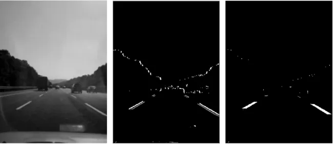
2.4 Lane Probed Algorithm
From Figure 2.5, we can see that the lane pattern is symmetry. So, we use this attribute to develop an algorithm to keep the problem lane marker. We call it lane probed algorithm. The main concept is, if we probed a series positive edge pixel following a series space pixel and negative pixels with some proportions, we then regard that as a lane marker. In our system, we assume that a series pixel is smaller than 3 pixels. Then we stuff white color in the positive and negative lane edges for subsequence algorithm operation. The Figure 2.4 (c) shows that the image processed with lane probe algorithm will get a clear lane image. It will help us to calculate the road area later in this chapter. Following is the pseudo code of lane probe algorithm.
for(Y = m_ImgTop; Y<m_ImgBottom; Y++){
addr = Y*ImgWidth;
Count3 = 0;Count1 = 0;Count2 = 0;
strX=-1; endX=-1;
for(X = ImgWidth/2; X<ImgWidth; X++){
if(Count1!=0){
if(pGrayImg[addr+X]==128){
Count1++;
if(strX==-1) strX = X;
}
else if(pGrayImg[addr+X]==0){
if((Count1>=2)&&(abs(Count1-Count3)<=2)){
endX=X;
break;
}
Count2++;
if(Count2>3){
Count3 = 0;
Count1 = 0;
Count2 = 0;
strX=-1;
endX=-1;
} } else{
Count3++;
} } else{
if(pGrayImg[addr+X]==128){
Count1++;
} } }
if((strX!=-1)&&(endX!=-1)){
for(X=ImgWidth/2;X<strX; X++){
pGrayImg[addr+X] = 0;
}
for(;X<endX; X++){
pGrayImg[addr+X] = 255;
}
for(;X<ImgWidth; X++){
pGrayImg[addr+X] = 0;
} } else{
for(X=ImgWidth/2;X<ImgWidth; X++){
pGrayImg[addr+X] = 0;
} }
Count3 = 0; Count1 = 0; Count2 = 0;
strX=-1; endX=-1;
for(X = (ImgWidth/2)-1; X>=0; X--){
if(Count1!=0){
if(pGrayImg[addr+X]==128){
Count1++;
if(strX==-1) strX = X;
}
else if(pGrayImg[addr+X]==0){
if((Count1>=2)&&(abs(Count1-Count3)<=2)){
endX=X;
break;
}
Count2++;
if(Count2>3){
Count3 = 0;
Count1 = 0;
Count2 = 0;
strX=-1;
endX=-1;
} } else {
Count3++;
} } else{
if(pGrayImg[addr+X]==128){
Count1++;
} } }
if((strX!=-1)&&(endX!=-1)){
for(X=(ImgWidth/2)-1;X>strX; X--){
pGrayImg[addr+X] = 0;
}
for(;X>endX; X--){
pGrayImg[addr+X] = 255;
}
for(;X>=0; X--){
pGrayImg[addr+X] = 0;
} } else{
for(X=0;X<ImgWidth/2; X++){
pGrayImg[addr+X] = 0;
} }
}
(a) (b) (c)
Figure 2.4: (a) Original Image. (b) The image applied the lane filter. (c) The image processed with lane probe algorithm.
(a) (b) Figure 2.5: (a) Lane pattern. (b) Others
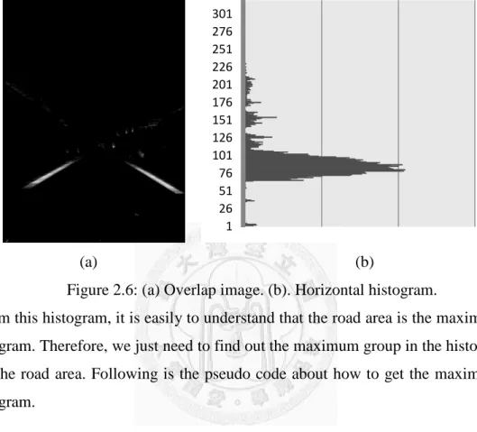
2.5 Road Area Conjecture
After the previous processes, we will use those processed images to conjecture the road area. In this thesis, we propose a histogram algorithm to conjecture the road area. At first, we overlap every image which was processed by lane probe algorithm. In our experiment experiences, overlaping 50 images is enough to do the conjecture. Figure 2.5 (a) is the result of overlapping 50 images. In this image we can see that, the lane was marked on the image very clearly. But there are still some noises. Maybe we can use some advanced algorithm to rule out these noises. However it is not efficient on mobile device, so we do not remove these noises
directly. We use statistic to vote the road area. Do a horizontal histogram on overlapping images is our counterplot. Figure 2.5 (b) is the histogram of figure 2.5 (a).
(a) (b)
Figure 2.6: (a) Overlap image. (b). Horizontal histogram.
From this histogram, it is easily to understand that the road area is the maximum group in the histogram. Therefore, we just need to find out the maximum group in the histogram and we can get the road area. Following is the pseudo code about how to get the maximum group in the histogram.
1 26 51 76 101 126 151 176 201 226 251 276 301
for(s=0; s<Length; s++) { AddValue = 0;
for(e=s; e<Length; e++) { AddValue += pProject[e];
if(pProject[e]==0) break;
}
if(g<40) {
group[g].add_value = AddValue;
group[g].top = s;
group[g].bottom = e;
if(AddValue>MaxGrup) { MaxGrup = AddValue;
*pTop = s;
*pBottom = e;
mg = g;
} g++;
}
for(;e<Length;e++) if(pProject[e]!=0) break;
s=e;
}
unsigned long mean=0;
for(s = *pTop; s<*pBottom; s++) { mean += pProject[s];
}
mean = mean/(*pBottom - *pTop);
for(e = *pBottom; e>=*pTop; e--){
if(pProject[e]>mean) break;
}
*pBottom = e;
Chapter 3
Accurate Lane Detection
We have proposed some lane filters and extraction lane algorithms. However it still has a lot of noise information in the processed image. Most of papers use a second order model to model the lane. This is:
y = a + a x + a x (3.1) They always use least square fitting to find the coefficients. If the image just has lane markers and this algorithm can find the correct lane fit. But, if there are too many noise markers in the image such as car shadow, traffic signs, guardrail and so on, this kind of fitting should be failed. So, these fitting like papers are not accurate practical in our project. The other people use hardware to do the brute force voting the lane curve. But, this kind of algorithm is very expensive and hard to implement on the embedded system. In this chapter, we proposed a smart voting system which is merges with simple linear regression.
3.1 Image Normalization
From Figure 2.4(c), we can see that if we just use filter to treat the image, it is hard to extract the lane marker cleanly. Some papers used Gaussian Filter with Sobel Filter or get its gradient in image. Of course, it can get a good lane marker image, but they are very expensive for CPU. We have done an experiment which deal with a gradient process on an image with 240x320 and it consumed 220 ms in our system. So, we propose that using a color information to pick up lane and car object and do the filter process in chapter 2.2. It is very efficient, because we can do the color probe at the color transform stage conveniently. But, the color range is hard to be defined. There are too many factors cause the image with different color temperature, contrast, brightness and saturation. Therefore, we need to normalize the input image at first. Following is our normalization algorithm.
S = 255 × ∑ (3.2) l k = 0,1,2, … ,255
l nj : Number of pixel with intensity j.
l n: Total number of pixels.
l For every pixel if I(im,i,j) = k then I(imhe,i,j) = Sk
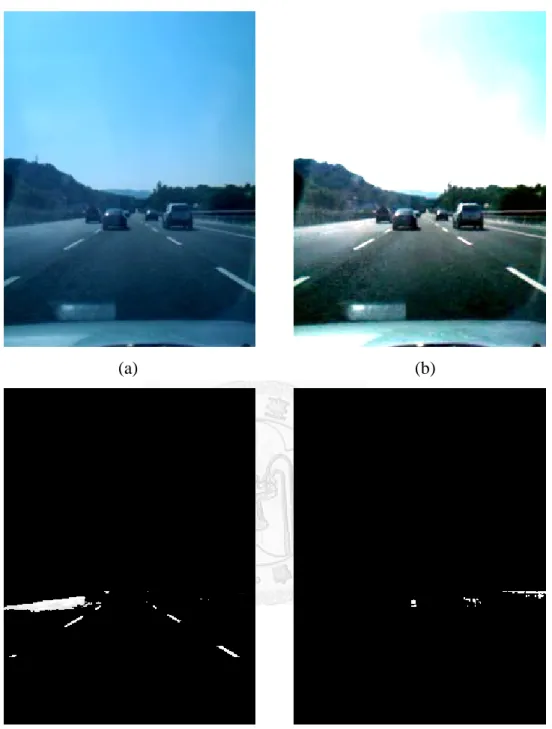
In our algorithm, we do not use full image to do the normalization as we worry about the lane color and black shadow. If we use full image to do the normalization process, the most white and most black should not appear in road area. And therefore result in the lane color or car shadow hard to be detected. For the reason, we will just use the road crop area to do the normalization analysis. In Figure 3.1 (a) is the original image. We can see that the image is partial blue and the lane is not white in the image. In Figure 3.1 (b) is the normalized image.
The lane in the image is pure white and the shadow is the most black. That is helpful for us to use color information to do the lane and car detection.
(a) (b) Figure 3.1: (a) Original image. (b) Normalization image.
3.2 Lane and Vehicle Detection
The gray level image is one of the most important source for computer vision, because it is easily to be done with some edge detections. In this system, we need to make the best of CPU resource. We think that we should do something in the color transform stage at the same time. Using object’s color information to do the object detection is a good choice in this system.
In Taiwan, lanes are with white, yellow and red color. Vehicle has deep black shadow in the daytime [8]. In this thesis, we propose to use HSV color domain to do the color object detection. Using RGB color domain to do the color object detection is hard to define what is white, yellow or red. If used HSV color domain, we can define that white is V bigger than 192 and S is small than 64. Yellow is S bigger than 60 and H between 40 and 60. Red is S bigger than 60 and H between 350 and 10. Deep black is V smaller than 50 and S bigger than 86. We can get the gray scale image from V and separate the lane object and vehicle object images at this stage conveniently. Figure 3.2 shows that we can separate the vehicle and lane with color transform at the same time.
(a) (b)
(b) (d)
Figure 3.2: (a) Original image. (b) Normalization image. (c) Separated lane image from normalization image. (d) Separated vehicle image from normalization image.
3.3 Extract Lane
In this stage, we need to extract lane markers as much as possible as we will use these lane markers to do the linear fitting. Otherwise, if the markers are not clear enough the result will be wrong. In Figure 3.2 (b), the separated lane image is not clear enough because it contains the wrong markers caused by halo and reflected light. Hence, we need to apply lane filter and lane probed algorithms on the separated lane images. But the lane probed algorithm in this stage has some difference. We do not fill in the gap with negative and positive edge.
That will cause too many lane markers and lead the linear fitting hard to work on embedded system. Thus, we just keep the middle point of negative and positive edge. Figure 3.3 (a) is an extracted lane image.
3.4 Lane Model
The application in this thesis, lane fitting is an auxiliary function. We used lane to find the front vehicle and driving shift. The lane in the high way is closed to straight line even if in curve. If we just went to find front vehicle, the absolute lane fitting is not necessary. In addition, the calculation power of RISC CPU is very week for quadratic curve operation.
Therefore, we just used a linear equation to do the lane fitting. And in our experiment, we proved that a linear equation is good enough in this project. Following is our lane model.
y = ax + b (3.3) After got the separated lane images, we collected the potential lane pixels and did the least squares fitting to derivate the lane model. In this case, the two sets of linear equations Lr and Ll could be then determined by using the information of the right and left lane coordinates.
Take the right lane markings for example, let the extracted points be a set of N observations {(x, y), i = 1,2, … , N}. The straight-line equation (3.4) used to fit these points.
y = ax + b (3.4) The error function (3.7) is a smooth non-negative function with two parameters a and b will have a global minimum at the point (a, b) where (∂E/ ∂a = 0) and (∂E/ ∂b = 0).
E = y − y (3.5) E = y − (ax + b) (3.6) E = ∑ (y − ax − b) (3.7)
= 2 ∑ (y − ax − b)(−x) = 0 (3.8)
= 2 ∑ (y − ax − b)(−1) = 0 (3.9)
−1 × ∑ x y + a × ∑ x + b × ∑ x = 0 (3.10)
−1 × ∑ y + a × ∑ x + b × ∑ i = 0 (3.11)
a × ∑ x + b × ∑ x = ∑ x y (3.12) a × ∑ x + b × N = ∑ y (3.13)
These equations are nicely represented in matrix form. The parameters of the best line are found by solving the equation (3.14).
∑ x ∑ x
∑ x N ab = ∑ x y
∑ y (3.14)
Following shows the liner fitting result:
(a) (b)
Figure 3.3: (a) Lane marker image. (b) Linear fitting result.
3.5 Slope Histogram
Using least squares fitting to derivate the lane model is an efficient way. But this method should be with a necessary condition that a clear lane separated image is required. If we do not get a clear lane separated image like in Figure 3.4 (a) then we will get a wrong linear fitting result such as in Figure 3.4 (b). However, to get an absolute clear separated lane image needs a lot of preprocess on the input images. It is very consumption of the resource on smart phone system. Thus, we did not use linear fitting to find the lane model at the decision stage. Instead, we used the vote algorithm to get the lane model.
In this section, we need to do some things for the accelerating vote speed. We think that, if user set the camera up at the cabin and the view angle is fixed, the slop of right and left lanes is located at two normality values if the driver drives at the middle of the lane. We did the statics of factor “a” in equation (3.3) with some frames and get the slope “a” which is the most voted. Then we defined two new linear equations with capital letter “A” and “B” which is means the maximum voted slope on left lane and right lane.
y = Ax + by = Bx + c (3.15)
After getting these two lane model equations, we need to redefine the road area by equation (3.15). The top boundary “Top” is such as following equation.
Top = A × + b. (3.16) And bottom “Bot” is such as following equation.
Bot = min (b, c) (3.17)
3.6 Lane Voting
In this thesis, we proposed to use the lane voting algorithm to get an accurate lane model equation. The benefit of lane voting algorithm is that we do not need to get an absolutely clear lane marker image but can get accurate lane model equation easily. The first stage is only to get lane marker image and following with the follow chart of getting pre-process lane image for the lane voting.
Figure 3.4: The flow chart of pre-process lane image for lane voting.
In Figure 3.4, the stages of “Image Normalization”, “Lane Detection in HSV Color Domain” and “Apply Lane Filter” are related to previous chapters.
After getting the lane mark images, we can start to do the lane voting process. From chapter 3.4, we have got two equations. One is the left lane model and another is right. The idea is to use these equations to scan full lane mark image and take the maximum matched equation to be the lane model equation. (Figure 3.5)
Get Color Image
Image Normalization
Lane Detection in HSV Color Domain
Apply Lane Filter
.
Figure 3.5: (a) Matching left lane. (b) Matching right lane.
. (a)
(b)
Figure 3.5: (a) Matching left lane. (b) Matching right lane.
.
.
…
.
… … …
Figure 3.5: (a) Matching left lane. (b) Matching right lane.
After getting the maximum matching, we matched lane model is just the closest equation
we fix the parameter “b” in the equation (3.3) and do some addition parameter “a” to get potential maximum match.
the maximum matching, we need to do some angle fine tun matched lane model is just the closest equation to the real lane marker. In our fine tune
in the equation (3.3) and do some additions and subtraction to get potential maximum match. In Figure 3.6 is our matching result.
Figure 3.6: Lane voting result.
need to do some angle fine tunings. The real lane marker. In our fine tune process,
and subtractions on igure 3.6 is our matching result.
The vehicle detection is very important in this system.
in the image demands a complexity algorithm to do it. In this algorithm to detect a vehicle in the
4.1 Detect Vehicle by the Shadow
In the chapter 3.1, we separated
stage. In this chapter, we need to do more calculation to extract the vehicle at the front. We do not care the neighborhood vehicle
up of the lane models. The blue area in the following
4.2 C-means
We used shadow to conjecture shape feature so it is hard to use
the shape. Here, we use C-means to decide the position of algorithm.
V(x, y) = ∑ xi , ∑
N: The markers of vehicle in the searching area.
In our system, we just need to get the y position. So, we can simplify the equation (4.1) as following.
V(y) = ∑ yi
Figure 4.2 is our search result.
Chapter 4
Vehicle Detection
ehicle detection is very important in this system. A robust vehicle detection process a complexity algorithm to do it. In this thesis, we propose
in the front, but it bases on the searching assistance
separated the land and vehicle images at image color transform stage. In this chapter, we need to do more calculation to extract the vehicle at the front. We do
t care the neighborhood vehicles but just the front one. So, the search area is just in the up of the lane models. The blue area in the following Figure 4.1 is the searched area.
Figure 4.1 Vehicle searched area.
conjecture the front vehicle, however the shadow t is hard to use feature definition to make decision about the
means to decide the position of the front vehicle.
yi N: The markers of vehicle in the searching area.
In our system, we just need to get the y position. So, we can simplify the equation (4.1) as
A robust vehicle detection process , we proposed an easy assistance at pre-chapter.
at image color transform stage. In this chapter, we need to do more calculation to extract the vehicle at the front. We do but just the front one. So, the search area is just in the fence
igure 4.1 is the searched area.
the shadow do not have any to make decision about the authenticity of front vehicle. Following is our
(4.1)
In our system, we just need to get the y position. So, we can simplify the equation (4.1) as
(4.2)
(a) (b) Figure 4.2: (a) Real image. (b) Vehicle markers image.
Chapter 5
Auto Calibration
Using computer vision to detect distance from 2D image in previous papers is very complex for users. Generally, it is hard to detect image from 2D image directly. People need to provide camera parameter and the coordinates of camera setup. We provide a user friendly distance measure method assists with GPS.
5.1 GPS
GPS is a common device in the smart phone now. It can provide the coordinate of longitude and time information. We can get the speed and time information through Microsoft standard API and use it to do the automatic 2D distance measure calibration.
5.2 Auto Calibration
In this thesis, we proved an algorithm to do the distance measurement. This algorithm has an important supposition that is front vehicle is const speed cruise. For this reason, we cannot calibration it immediately, we need to static the parameters set which derived from the algorithm in a while. Finally, we chosen the maximum statistic one to be the calibration result.
The accuracy of GPS is not very exact. We do the calibration at once in one second interval.
The parameters got in an image are time, speed and vehicle coordinate in the image. Figure 5.1 is the sketch map of the got parameters.
Figure 5.1: The sketch map of calibration parameter
By the anti-perspective projection, people can map points on the 2D plane to 3D world system. But in our system, users do not need to input camera parameter and setup coordination.
It is hard to do the mapping directly by this theory. In Figure 5.2, we can see that the x-axis project to y-axis on 2D plane is approaching to the parabolic curve. Thus, we propose to use parabolic curve (Y − b) = aX to get the mapping of 2D plane in coordinate with 3D world coordinate system for distance measuring.
Figure 5.2: Perspective projection of ground plane and the relationship of parabolic curve.
Following is our derivation about how to get the parabolic curve approach from three images with 1 second interval by themselves.
Image t1 front vehicle position Image t2 front vehicle position
Lane Y1
Y2
Image time 1( t1) with speed V1 Image time 2(t2) with speed V2 1 second
Maximum distance
Minimum distance
Max_Y
Min_Y
Image plane Optical center
Optical axis
Ground plane
Parabolic curve
0 Y
X
Step1. We can get the acceleration “A” by the equation (5.1).
A = (5.1) Step2. The shift of our car “S” is got by equation (5.2).
S = V1 + A
S = V2 + A (5.2) Step3. Then solve the following equation (5.3) to get the parameter “a” and “b” in the
parabolic curve equation (Y − b) = aX .
( ) ( )
(5.3)
=>
a =( ) ( )
a =( ) ( ) (5.4)
=>( ) ( ) =( ) ( ) (5.5)
=> b = (5.6)
In the calibration stage, we needed to do the parabolic curve approach for a while.
Because we expected that the front vehicle was with a constant speed and we had the acceleration. If not fitting in these conditions, the result will be wrong. Therefore, we need to do the approach to static the parameter “a” and “b” for finding the maximum candidate to be our parabolic curve approach result.
Chapter 6
Distance Measurement
After dealing with the parabolic approach curve parameter “a” in the front chapter, we now can get front vehicle distance easily. The decision stage is just to find the front vehicle in the sequencial input images and use the following equation (6.1) to get the real world distance.
X = ( ) (6.1) Figure 6.1 show that we can measure the distance of front car is 120 meter.
Figure 6.1: The example of front car distance measuring result.
Finally, using this distance to make a decision and do some warning alarms to driver when the car is too close to the front vehicle. In our implement, we can make a decision in 100 milliseconds. This should good enough to help driver to avoid some overtaking collision danger.
Chapter 7
Experiment
The aim of this thesis is to build up a Driver Assistance System which is suitable for mobile devices. Currently there are four smart phone systems on the market Windows Mobile, RIM, iPhone and Android. Though iPhone has a complete develop API supporting and well performance but it is belong to high-end smart phone. RIM is just popular at Europe and the developed tools are not very complete. Android was not release when we created this project.
So we chose Windows Mobile system to be our target developing system.
7.1 Hardware Environment Description
Even though Microsoft has define a camera module access path from Direct Show after windows mobile 5.0, but there are still not many window mobile system smart phones supporting this feature. After having done the many tests, we just found that the HTC has supporting Direct Show completely. Therefore, we chose HTC Touch Diamond P3702 to be our developing environment. Figure 7.1 is its appearance.
Figure 7.1: HTC Touch Diamond P3702
Table 7.1 shows the detailed description of the system, it consists of the processor, memory, camera and GPS.
Table 7.1: Hardware system information.
Component Information
CPU Qualcomm® MSM7201A™ 528 MHz
OS Windows Mobile® 6.1 Professional
Memory RAM: 192MB DDR SDRAM
Display VGA (480x640) 2.8”
Camera 320 Mega Pixels with auto focus
GPS GPS and A-GPS
7.2 Software Environment Description
Microsoft has a complete windows mobile developer center website.
http://msdn.microsoft.com/en-us/windowsmobile/default.aspx Our software system is listed at following table 7.2.
Table 7.2: Software system information.
Component Information
OS Windows Vista SP1
IDE Visual Studio 2008 Professional with SP1
SDK Windows Mobile 6 SDKs
Synchronization Windows Mobile Device Center .
7.3 Get Image by Direct Show
Getting image from camera is very hard from the previous to the present. Generally, the smart phone developer needed to get the camera SDK from camera vender for camera application development. But it is not release to end users. So we need to get image by Direct Show. Direct Show is a convent technique, users only need to assemble the components and finish its work. In Windows Mobile 6 SDKs, it supported “Camera Driver ” and “Video Capture” filters for getting image from camera. But, unfortunately it just has “Video Render” filter for display. It lacked “Video Grab” filter for grabbing video from the pipe. Therefore, we need to create a “Grabber” filter by myself and insert it to the filters link. Figure 7.2 shows the framework of video flow.
Figure 7.2: The flow chart of our Direct Show filters link.
7.4 Experiment Result
Figure 7.3 shows the result of the online front vehicle detection. The figure 7.3 (a), (b), (c) and (d) are sequencial images. The green horizontal lines in the camera image are the tracking of the front vehicle. The red oblique lines in the camera image are the lane detection markers.
They provide the information of process stage, frame rate, speed, front vehicle distance and got satellite number. We can confirm that we processed a frame in 100 milliseconds by the frame rate. The front car in the sequence images can show that our distance measurement algorithm is match to the front car revealing in the images.
Camera
Camera Driver (DMO)
Video Capture (CLSID_Vide oCapture)
Grabber
Video Render
LCD
Process the image
(a) (b)
(c) (d) Figure 7.3: Front vehicle tracking and distance measure.
(a) 120 meters away from the vehicle in front.
(b) 132 meters away from the vehicle in front.
(c) 117 meters away from the vehicle in front.
(d) 106 meters away from the vehicle in front.
Chapter 8
Conclusions and Future Works
This study provided a driver assistance system on the smart phone. The experiment demonstrated that the algorithm was workable and had enough accuracy. But it still has many defects such as it could just be used in daytime and high way. The GPS latency and accuracy will cause the system collected with wrong results. The bad weather and lane marker will lead to fail decision. The non vehicle shadows lead vehicle to judge in the mistake. But, by the limitation of the computing power, we could just reach to this performance. If the computing power is good enough, we can design a better shadow pick out algorithm for fake shadows. If the memory is enough, we can keep the pre-frames in the memory to overcome GPS latency. The decision system and training system are required to be redesigned for nighttime as well.
Reference
[1] S. K. Kemue, “LANELOK: Detection of lane boundaries and vehicle tracking using image-processing techniques – Parts I and II” SPIE Mobile Robots IV, 1989.
[2] K.C. Kluge, YARF: An Open-Ended Framework for Robot Road Following, PH.D Thesis, Carnegie Mellon University, 1993.
[3] K.C. Kluge, “Extracting road curvature and orientation from image edge points without perceptual grouping into features,” Proceedings of the Intelligent Vehicle ’94 Symposium, pp.109-114, 1994.
[4] D. Pomerleau and T. Jochem, “Rapidly Adapting Machine Vision for Automated Vehicle Steering,” IEEE Expert, 11, (2), pp.302-7, April 1996.
[5] K. C. Kluge, “Performance evaluation of vision-based lane sensing: some preliminary tools, metrics and result,” IEEE Conference on Intelligent Transportation System, 1997.
[6] K. Y. Chiu and S. F. Lint, “Lane Detection using Color-Based segmentation”, Department of Electrical and Control Engineering, National Chiao-Tung University, Taiwan, ROC.
[7] S. Terakubo, et. al., “Development of an AHS safe driving system,” SEI Technical Review, no. 45, pp.71-77, 1998.
[8] M. Y. Chern, B. Y. Shyr, "Locating nearby vehicles on highway at daytime based on the front vision of a moving car," Proceedings of Robotics and Automation, vol. 2, 2003, pp.
2085 - 2090.