以分子動態模擬研究PTT(聚對苯二甲酸丙二脂)結晶初期行為

(1)

國立臺灣大學工學院化學工程學系碩士論文

Department of Chemical Engineering College of Engineering

National Taiwan University Master Thesis

以分子動態模擬研究 PTT(聚對苯二甲酸丙二脂) 結晶初期行為

Early State Crystallization Process of Poly (Trimethylene Terephthalate) (PTT) Polymer

from Atomistic Molecular Dynamics Simulations

謝旻剛 Min-Kang Hsieh

指導教授：林祥泰博士 Advisor: Shiang-Tai Lin, Ph.D.

中華民國 97 年 7 月 July, 2008

(2)

(3)

誌謝

首先感謝口試委員諶玉真教授、黃慶怡教授及郭錦龍教授在百忙之中抽空前來參加我論文口試，感謝你們的指教及寶貴意見，讓我的論文增色不少。

畢業了，結束在台大六年的生活。多采多姿的大學生活，加上精實的研究生生活，成為我未來最有利的後盾。在這裡，學到的不只是專業的知識，更重要的是開闊自己的視野。分子模擬從只是引起我好其的電影《透明人》中的一個鏡頭，變成了研究的工具，變成我的專業能力之ㄧ。在林祥泰教授的引領之下，了解箇中的奧妙，更給了我不ㄧ樣的角度來看這個世界所發生的每一件事，感謝林教授的提攜、

教導，感謝您的協助完成本研究及碩士論文。也要感謝實驗室的每一個成員，感謝引我入門的小董學長，沒有你的棄而不顧，哪來我的迄而不捨。感謝阿伯的程式經驗分享，還有你耐心的聽我述說的研究，

並在關鍵的時還提供不錯的想法。感謝阿竹、崇民及旻璁學長。感謝小傑，小容容，一起修課的歡樂，一起在實驗室待到12 點。感謝舒潔，

展嘉和孟廷在熱力學上的分享，感謝穎銘學弟，感謝博宇學弟，感謝小學弟阿源，調參數很辛苦但要更努力，感謝在這兩來來幫過我的大家。

感謝家人，感謝父親默默的支持，感謝母親為我操心，雖然你一直問我高分子是不是生物；感謝妹妹承受比較的壓力，也恭喜你學業更上一層樓。感謝前女友的支持跟鼓勵，你的離開讓我跌入深淵後更無後顧之憂的勇往直前。

(4)

摘要

以分子動態模擬研究聚對苯二甲酸丙二脂(PTT)結晶初期行為。藉由模擬恆溫結晶及拉伸程序，我們證實結晶核前驅物(precursor of nuclei)的存在，並發現其成長主要受到高分子主鏈的旋轉能量(torsional energy)及分子間凡得瓦爾作用力(van der Waals interaction)的影響。我們成功預測聚對苯二甲酸丙二脂的玻璃轉移溫度(Tg)及熔點(Tm)，並發現在恆溫結晶程序中，結晶核前驅物的總量在這兩溫度區間快速增加，接著維持週期性波動。此外；高分子主鏈藉由旋轉的分式重新排列，趨向結晶的結構。在拉伸程序中，有向性的晶核前驅物(oriented precursor)的總量大大的提升。系統中，高分子主鏈的旋轉角度分佈快速變成直鏈狀(trans-trans-trans-trans)構形。並在個別的有向性的晶核前驅物中，發現兩組旋轉角趨向結晶結構的轉變速率不同。其內部結構成長的三個因素:高分子鏈段的個數、旋轉角度(torsional angle)及排列緊密程度相互競爭或妥協，使結晶前趨物結構趨向結晶結構。由結果支持結晶前趨物在結晶初期扮演重要的角色。

(5)

Abstract

Atomistic molecular dynamics simulations are performed to study the initial crystallization process of poly(trimethylene terephthalate) (PTT). The structure development of ordering structures (nuclei precursors) in the isothermal and stress-induced crystallization process has been observed in our simulations. The formation of nucleus precursors is found to be driven mainly by the torsional and van der Waals forces. The thermal properties, such as the glass transition temperature (Tg) and the melting temperature (Tm), determined from our simulation are in good agreement with experimental values. In isothermal processes, it is found that, between these two temperatures, the amount of precursors quickly arises during thermal relaxation period soon after the system is quenched and starts to fluctuate afterwards.

The variation of precursor fraction with temperature exhibits a maximum between Tg

and Tm, resembling temperature dependence of crystallization rate for most polymers. In addition, the backbone torsion distribution for segments within the precursor preferentially reorganizes to the trans-gauche-gauche-trans (t-g-g-t) conformation, the same as that in the crystalline state. On the other hand, during stress-induced crystallization, the amount of stress-induced precursor increases in all regions of temperature. The torsional distribution of the polymer backbone for segments rapidly rearrange to the t-t-t-t conformation in bulk phase. Within oriented precursors, the response of the torsional angle induced by stress is faster than that only induced by thermal stimulation, especially trans in φ1(the transition rate of trans state in φ1 is faster than that of gauche state in φ2). Within precursors, three factors: size, torsional angle and degree of packing found to compete/compromise during crystallization. As a consequence, we believe that the precursors play an important role as an incubator for the formation of the more compact and ordered nuclei.

(6)

Catalog

口試委員會審定書... i

誌謝... ii

摘要... iii

Abstract ... iv

Catalog... v

Catalog of Table... ix

Catalog of figure ... xi

1 Introduction... 1

1.1 Kinetics of polymer crystallization ... 1

1.2 Existence of Precursors ... 3

1.3 Stress-induced crystallization... 5

1.4 Polymer of PTT ... 8

1.5 The transition of conformation during crystallization... 15

1.6 Motivation ... 17

2 Theory ... 19

2.1 Molecular dynamic simulation ... 19

2.2 Algorithm ... 19

2.3 Force field... 20

2.3.1 Bond energy... 21

2.3.2 Angle energy ... 21

2.3.3 Torsion energy... 22

2.3.4 Inversion energy ... 22

2.3.5 Coulomb interaction ... 22

2.3.6 Van der Waals interaction ... 23

(7)

2.4 Thermal behavior... 25

2.4.1 Glass transition temperature ... 25

2.4.2 Melting temperature ... 25

2.5 Mechanical properties ... 28

2.6 Definition of the segment packing structure (precursor structure)... 29

2.7 Definition of the torsion angle state ... 30

2.8 Other properties ... 31

2.8.1 Radial distribution function... 31

2.8.2 Persistence length ... 32

2.8.3 Orientation factor... 32

3 Computation method and detail... 34

3.1 Method... 34

3.2 Model building ... 35

3.2.1 Amorphous sample ... 35

3.2.2 Crystal sample ... 36

3.2.3 Semi-crystal sample... 36

3.3 Ensemble and control detail ... 41

3.4 Force field validation... 42

3.4.1 Crystal structure properties and torsional angles... 42

3.4.2 Thermal properties... 42

3.4.3 Mechanical property... 43

3.5 Simulation process... 48

3.5.1 Iso-thermal crystallization process ... 48

3.5.2 Stress-induced crystallization process... 49

4 Isothermal Crystallization ... 51

(8)

4.1 Bulk properties ... 51

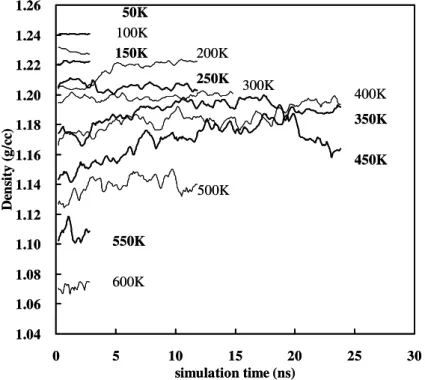
4.1.1 Density... 51

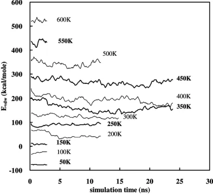
4.1.2 Energy... 51

4.1.3 Discussion... 56

4.2 Structure development in PTT upon quenching... 57

4.2.1 Precursor fraction ... 57

4.2.2 Degree of order of the system ... 60

4.3 Structure development within Nucleus precursor ... 63

4.3.1 Structure identification ... 63

4.3.2 Radial distribution function... 65

4.3.3 The average size of precursor... 70

4.3.4 Torsion angle distribution... 70

5 Stress-Induced Crystallization... 75

5.1 Bulk properties ... 75

5.1.1 Density... 75

5.1.2 Energy... 75

5.2 Structure development of the PTT upon drawing ... 84

5.2.1 Precursor fraction ... 84

5.2.2 Degree of Order... 89

5.2.3 Torsional angle transition ... 89

5.3 Structure development within oriented precursor. ... 103

(9)

5.3.1 Structure identification ... 103

5.3.2 The RDF, average size, and tosional angle of precursors ... 105

6 Conclusion ... 118

Appendix A... 120

Appendix B... 124

Appendix C... 128

Reference ... 139

(10)

Catalog of Table

Table 1.1 The Avrami parameters for crystallization of polymers... 3

Table 1.2 Summary of Avrami exponent in isothermal process. ... 13

Table 1.3 Summary of model’s exponent in non-isothermal process. ... 13

Table 1.4a The kinetic crystallizability of non-isothermal process analysis by Ziabicki model[44]. ... 14

Table 1.4b The kinetic crystallizability of non-isothermal process analysis by Ziabicki model[43]. ... 14

Table 1.5 The identification of IR bands corresponding with propylene glycol segments. ... 17

Table 3.1 Comparison of the lattice parameters, density, and torsional angles of crystalline PTT... 44

Table 3.2 Young’s modulus of PTT at different condition... 47

Table 3.3 The number of independent samples used to study stress-induced crystallization. ... 49

Table 3.4a The simulatoin time for isothermal relaxation of PTT after different draw ratios at a constant draw speed of 1x10⁹ s^-1... 50

Table 3.4b The simulation time for isothermal relaxation of PTT after different draw ratios at constant draw speeds of 1x10¹⁰ s^-1 and 1x10¹⁰ s^-1. ... 50

Table 4.1 The number and size of individual precursors identified in isothermal crystallization. ... 64

Table 5.1 The fraction of precursor with draw speed at 1x10⁹s^-1. ... 86

Table 5.2 The fraction of precursor with draw speed at 1x10¹⁰s^-1. ... 87

Table 5.3 The fraction of precursor with draw speed at 1x10¹¹s^-1. ... 88

Table 5.4 The index of torsional angle with draw speed at 1x10⁹s^-1. ... 98

(11)

Table 5.5 The index of torsional angle with draw speed at 1x10¹⁰s^-1... 99

Table 5.6 The index of torsional angle with draw speed at 1x10¹¹s^-1... 100

Table 5.7 The number and size of individual precursors identified in stress-induced crystallization with draw speed 1x10⁹s^-1. ... 104

Table 5.8 The number and size of individual precursors identified in stress-induced crystallization with draw speed 1x10¹⁰s^-1... 104

Table 5.9 The number and size of individual precursors identified in stress-induced crystallization with draw speed 1x10¹¹s^-1... 105

Table A.1 The definition of each atom type in atomic model... 120

Table A.2 The value of parameters of band energy in our simulation. ... 121

Table A.3 The value of parameters of angle energy in our simulation. ... 121

Table A.4 The value of parameters of torsion energy in our simulation... 122

Table A.5 The value of parameters of inversion energy in our simulation... 122

Table A.5 The value of parameters of Van der Waals interaction in our simulation.... 123

Table B.1 The number and size of individual precursors identified in MD simulations. (27x8) ... 124

Table C.1 The number and size of individual precursors identified in stress-induced crystallization with draw speed 1x10¹⁰s^-1. (27x14) ... 128

Table C.2 The number and size of individual precursors identified in stress-induced crystallization with draw speed 5x10¹⁰s^-1. (27x14) ... 129

Table C.3 The number and size of individual precursors identified in stress-induced crystallization with draw speed 1x10¹¹s^-1. (27x14) ... 129

(12)

Catalog of figure

Figure 1.1 Stress-draw ratio curve of melt-quenched amorphous PTT film during uniaxial drawing around Tg. [18]... 7 Figure 1.2 Crystallinity changes as a function of draw ratio for uniaxially and biaxially drawn PTT films. [18] ... 8 Figure 1.3 Chemical structure of a repeating unit of PTT (a) and a fragment (4

repeating units) of the PTT chain (b). Carbon atoms are shown in grey, oxygen in red, and hydrogen in yellow. The green cylinders connecting the centers of adjacent aromatic rings are taken as elementary segments in the precursor analysis. ... 9 Figure 2.1 Comparison the energy barriers distribution with rotating torsion angles.

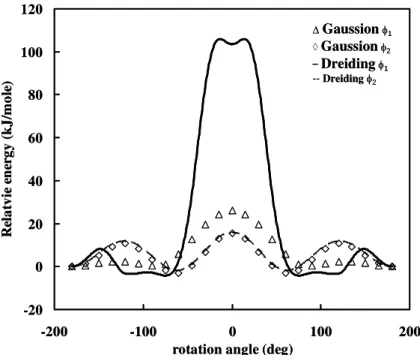
Check the results of dreiding force field in φ1 (solid line), and φ2 (dash line) against that of quantum mechanics using the B3LYP functional and 6-31G** basis set in Gaussian 98 in φ1 (triangle), and φ2 (diamond)... 24 Figure 2.2 Modification the energy barriers distribution with rotating torsion angle of φ1.

Accept the result of parameter n = 3, K = 2, and d= -1 to use in torsion energy... 24 Figure 2.3 General variations in (a) volume, V, (b) enthalpy, H, and (c) and storage

shear modulus, G’ as function of temperature. Also show (d) volume expansion coefficient, α, and (e) heat capacity, Cp, which is the first derivation of V and H, respectively with respect to temperature, and (f) the loss shear modulus, G”. [2]... 26 Figure 2.4 The viscoelastic behavior of amorphous polymer (solid line), crystalline

polymer (dashed line), and cross-linking polymer (dotted line) as function of temperature. There are five regions shown as (1) glassy region, (2) glass transition region, (3) rubbery plateau region, (4) rubbery flow region, and (5) liquid flow region.[2] ... 27

(13)

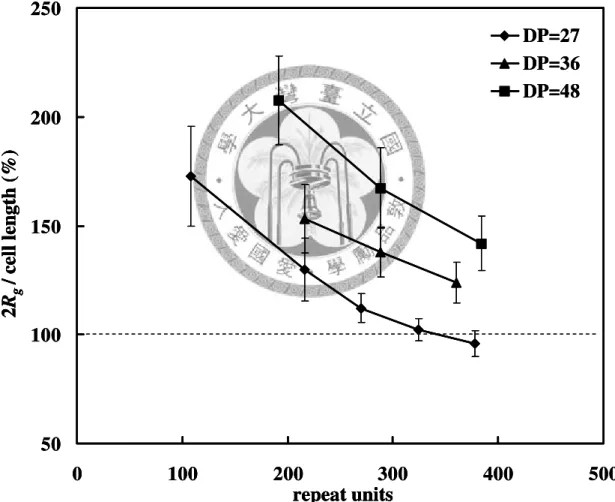
Figure 3.1 The flowchart of the calculation process... 35 Figure 3.2 The radius of gyration (Rg) of PTT chains as the function of repeat units.. 37 Figure 3.3 An amorphous structure at 600K. The system contains 4 chains of PTT

molecules, each having a degree of polymerization of 27 overall 2708 atoms. The cell parameter: a = 31.93Å, b = 31.93Å, c = 31.93Å, α= 90.00(deg), β= 90.00(deg), γ = 90.00(deg), and density is 1.06 g/cc... 38 Figure 3.4 A crystalline structure. The model contains 8 (2x2x2) atomic lattice cells, 4 chains of PTT molecules, each having 4 repeat units, overall 400 atoms. The cell parameter: a = 8.66Å, b = 12.56Å, c = 37.39Å, α= 101.66(deg), β= 90.00(deg), γ = 110.11(deg), and density is 1.47 g/cc. ... 39 Figure 3.5 An equally semi-crystal structure with Xc=18%. The model contains 25

chains of PTT molecule, each having a degree of polymerization of 4, overall 2550 atoms. The cell parameter: a = 21.96Å, b = 31.53Å, c = 39.35Å, α= 90.00(deg), β=

90.00(deg), γ = 90.00(deg), and density is 1.33 g/cc... 40 Figure 3.6 The density variation of PTT upon cooling and heating. The 600K

equilibrated sample cooled to 50K (open square) and 50K equilibrated sample heated to molten state (open circle). Each process was performed by step changes of temperature of 25K after 25ps... 45 Figure 3.7 The plot of the stress and strain curve. In all case, the slope of three lines is uniform. The technique of black average (3% of stain) used in data analysis results in the data shown form -1.5% to 1.5%. This example is drawn with draw speed 1x10¹⁰s^-1 in x-direction at 200K... 46 Figure 3.8 The calculated Yonug’s modulus is a function of the temperature and draw

speeds. The average curve considers all draw speeds. ... 46 Figure 3.9 The cooling and iso-thermal crystallization processes... 48

(14)

Figure 4.1 The time evolution of density during relaxation at different temperature.... 52 Figure 4.2The time evolution of kinetic energy... 52 Figure 4.3 The time evolution of potential energy during relaxation at different

temperature... 53 Figure 4.4 the time evolution of bond energy during relaxation at different temperature.

... 53 Figure 4.5 the time evolution of angle energy during relaxation at different temperature.

... 54 Figure 4.6 The time evolution of torsional energy during relaxation at different

temperature... 54 Figure 4.7 the time evolution of inversion energy during relaxation at different

temperature... 55 Figure 4.8 The time evolution of coulomb energy during relaxation at different

temperature... 55 Figure 4.9 The time evolution of van der Waals interaction during relaxation at different temperature... 56 Figure 4.10 The variation of the amount of the precursor (defined in eqationn 2.14)

with time at 350, 400, and 450K. (27x4)... 58 Figure 4.11 The variation of the average amount of the precursor (defined in eqationn

2.14) with temperature. (27x4)... 58 Figure 4.12 The variation of the amount of the precursor (defined in eqationn 2.14)

with time at 350, 400, and 450K. (27x8)... 59 Figure 4.13 The variation of the average amount of the precursor (defined in eqationn

2.14) with temperature. (27x8)... 59 Figure 4.14 The RDF of the quenched PTT state at 400K. ... 60

(15)

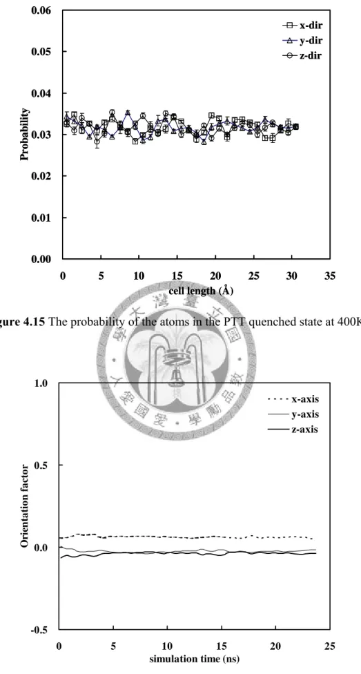
Figure 4.15 The probability of the atoms in the PTT quenched state at 400K... 61

Figure 4.16 The orientation factor in the PTT quenched state at 400K... 61

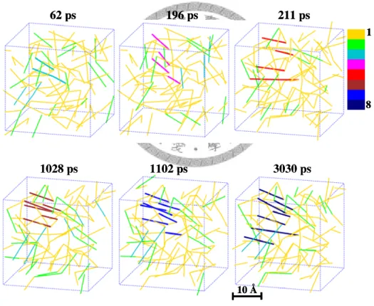
Figure 4.17 Illustration of the growth of nucleus precursor from melted state at 400 K. A color scale is used for better discrimination of the size of precursors... 64

Figure 4.18 The RDF of 1,4 carbon atoms in crystalline PTT structure during a heating process. ... 66

Figure 4.19 The RDF of precursor at 300K... 66

Figure 4.23 The time evolution of RDF intensity (4.11Å) (diamond) and the time averaged number of parallel segments contained in a representative precursor (triangle) at 300 K. ... 68

Figure 4.27 the backbone torsions <φ1> in trans (triangles) and <φ2> in gauche (circles) for segments in a precursor (closed symbols) and outside any precursor (open symbols) at 300 K. ... 71

(16)

Figure 4.28 the backbone torsions <φ1> in trans (triangles) and <φ2> in gauche (circles) for segments in a precursor (closed symbols) and outside any precursor (open symbols) at 300 K. ... 71 Figure 4.29 the backbone torsions <φ1> in trans (triangles) and <φ2> in gauche (circles) for segments in a precursor (closed symbols) and outside any precursor (open symbols) at 300 K. ... 72 Figure 4.30 the backbone torsions <φ1> in trans (triangles) and <φ2> in gauche (circles) for segments in a precursor (closed symbols) and outside any precursor (open symbols) at 300 K. ... 72 Figure 4.31 The percentage of these torsions in the trans and gauche states within all

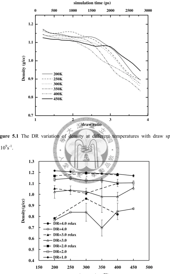
precursors. ... 73 Figure 5.1 The DR variation of density at different temperatures with draw speed

1x10⁹s^-1... 77 Figure 5.2 The temperature dependence of density at different DR with draw speed

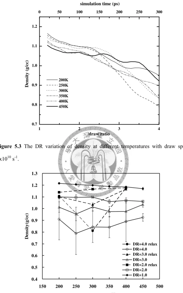
1x10⁹ s^-1... 77 Figure 5.3 The DR variation of density at different temperatures with draw speed

1x10¹⁰ s^-1... 78 Figure 5.4 The temperature dependence of density at different DR with draw speed

1x10¹⁰ s^-1... 78 Figure 5.5 The DR variation of density at different temperatures with draw speed

1x10¹¹ s^-1... 79 Figure 5.6 The temperature dependence of density at different DR with draw speed

1x10¹¹ s^-1... 79 Figure 5.7 The temperature dependence of torsional energy at different DR with draw

speed 1x10⁹ s^-1... 80

(17)

Figure 5.8 The temperature dependence of van der Waals interaction at different DR with draw speed 1x10⁹ s^-1... 80 Figure 5.9 The temperature dependence of torsional energy at different DR with draw

speed 1x10¹⁰ s^-1. ... 81 Figure 5.10 The temperature dependence of van der Waals interaction at different DR

with draw speed 1x10¹⁰ s^-1. ... 81 Figure 5.11 The temperature dependence of torsional energy at different DR with draw speed 1x10¹¹ s^-1... 82 Figure 5.12 The temperature dependence of van der Waals interaction at different DR

with draw speed 1x10¹¹ s^-1. ... 82 Figure 5.13 The draw speed dependence of density, torsional energy, and van der Waals interaction at different DR... 83 Figure 5.14 The temperature dependence of precursor fraction at different DR with

draw speed 1x10⁹ s^-1... 84 Figure 5.15 The temperature dependence of precursor fraction at different DR with

draw speed 1x10¹⁰ s^-1. ... 85 Figure 5.16 The temperature dependence of precursor fraction at different DR with

draw speed 1x10¹¹ s^-1... 85 Figure 5.17 The DR variation of RDF at (a) 400K, (b) 300K, and (c) 200K with draw

speed 1x10⁹ s^-1... 90 Figure 5.18 The DR variation of RDF at (a) 400K, (b) 300K, and (c) 200K with draw

speed 1x10¹⁰ s^-1. ... 90 Figure 5.19 The DR variation of RDF at (a) 400K, (b) 300K, and (c) 200K with draw

speed 1x10¹¹ s^-1... 91 Figure 5.20 The results of orientation factor at various temperatures and DR... 91

(18)

Figure 5.21 The percentage of trans state depends on temperature at DR=2, 3, and 4 with draw speed 1x10⁹ s^-1... 92 Figure 5.22 The percentage of trans state depends on temperature at DR=2, 3, and 4

with draw speed 1x10¹⁰ s^-1. ... 92 Figure 5.23 The percentage of trans state depends on temperature at DR=2, 3, and 4

with draw speed 1x10¹¹ s^-1. ... 93 Figure 5.24 The percentage of gauche state depends on temperature at DR=2, 3, and 4 with draw speed 1x10⁹ s^-1... 93 Figure 5.25 The percentage of gauche state depends on temperature at DR=2, 3, and 4 with draw speed 1x10¹⁰ s^-1. ... 94 Figure 5.26 The percentage of gauche state depends on temperature at DR=2, 3, and 4 with draw speed 1x10¹¹ s^-1. ... 94 Figure 5.27 The trans-to-gauche ratio in φ1 depends on temperature at DR=2, 3, and 4

with draw speed 1x10⁹ s^-1... 95 Figure 5.28 The trans-to-gauche ratio in φ1 depends on temperature at DR=2, 3, and 4

with draw speed 1x10¹⁰ s^-1. ... 95 Figure 5.29 The trans-to-gauche ratio in φ1 depends on temperature at DR=2, 3, and 4

with draw speed 1x10¹¹ s^-1. ... 96 Figure 5.30 The gauche-to-trans ratio in φ2 depends on temperature at DR=2, 3, and 4

with draw speed 1x10⁹ s^-1... 96 Figure 5.31 The gauche-to-trans ratio in φ2 depends on temperature at DR=2, 3, and 4

with draw speed 1x10¹⁰ s^-1. ... 97 Figure 5.32 The gauche-to-trans ratio in φ2 depends on temperature at DR=2, 3, and 4

with draw speed 1x10¹¹ s^-1. ... 97 Figure 5.33 The time evolution of RDF intensity (4.11Å) (diamond) and the time

(19)

averaged number of parallel segments contained in a representative precursor (triangle) at 200 K with draw speed 1x10⁹s^-1... 106 Figure 5.34 The backbone torsions <φ1> in trans (triangles) and <φ2> in gauche (circles)

for segments in a precursor at 200K with draw speed 1x10⁹s^-1. ... 106 Figure 5.35 The time evolution of RDF intensity (4.11Å) (diamond) and the time

averaged number of parallel segments contained in a representative precursor (triangle) at 200 K with draw speed 1x10¹⁰s^-1... 109 Figure 5.40 The backbone torsions <φ1> in trans (triangles) and <φ2> in gauche (circles)

for segments in a precursor at 200K with draw speed 1x10¹⁰s^-1. ... 109 Figure 5.41 The time evolution of RDF intensity (4.11Å) (diamond) and the time

averaged number of parallel segments contained in a representative precursor (triangle) at 300 K with draw speed 1x10¹⁰s^-1...110 Figure 5.42 The backbone torsions <φ1> in trans (triangles) and <φ2> in gauche (circles)

for segments in a precursor at 300K with draw speed 1x10¹⁰s^-1. ...110 Figure 5.43 The time evolution of RDF intensity (4.11Å) (diamond) and the time

(20)

averaged number of parallel segments contained in a representative precursor (triangle) at 400 K with draw speed 1x10¹⁰s^-1...111 Figure 5.44 The backbone torsions <φ1> in trans (triangles) and <φ2> in gauche (circles)

for segments in a precursor at 400K with draw speed 1x10¹⁰s^-1. ...111 Figure 5.45 The time evolution of RDF intensity (4.11Å) (diamond) and the time

averaged number of parallel segments contained in a representative precursor (triangle) at 200 K with draw speed 1x10¹¹s^-1...112 Figure 5.46 The backbone torsions <φ1> in trans (triangles) and <φ2> in gauche (circles)

for segments in a precursor at 200K with draw speed 1x10¹¹s^-1. ...112 Figure 5.47 The time evolution of RDF intensity (4.11Å) (diamond) and the time

for segments in a precursor at 300K with draw speed 1x10¹¹s^-1. ...113 Figure 5.49 The time evolution of RDF intensity (4.11Å) (diamond) and the time

for segments in a precursor at 400K with draw speed 1x10¹¹s^-1. ...114 Figure 5.51 The temperature dependence of the growth rate of precursor size with

different draw speeds...115 Figure 5.52 The temperature dependence of transition rate of torsional angle φ1 with

different draw speeds...115 Figure 5.53 The temperature dependence of transition rate of torsional angle φ2 with

different draw speeds...116

(21)

Figure A.1 The atomic position on the PTT polymer repeat unit. ... 120 Figure B.1 The time evolution of RDF intensity (4.11Å) (diamond) and the time

averaged number of parallel segments contained in a representative precursor (triangle) at 350 K. (27x8)... 125 Figure B.2 the backbone torsions <φ1> in trans (triangles) and <φ2> in gauche (circles) for segments in a precursor (closed symbols) and outside any precursor (open symbols) at 350 K. (27x8)... 125 Figure B.3 The time evolution of RDF intensity (4.11Å) (diamond) and the time

averaged number of parallel segments contained in a representative precursor (triangle) at 400 K. (27x8)... 126 Figure B.4 the backbone torsions <φ1> in trans (triangles) and <φ2> in gauche (circles) for segments in a precursor (closed symbols) and outside any precursor (open symbols) at 350 K. (27x8)... 126 Figure B.5 The time evolution of RDF intensity (4.11Å) (diamond) and the time

averaged number of parallel segments contained in a representative precursor (triangle) at 450 K. (27x8)... 127 Figure B.6 the backbone torsions <φ1> in trans (triangles) and <φ2> in gauche (circles) for segments in a precursor (closed symbols) and outside any precursor (open symbols) at 350 K. (27x8)... 127 Figure C.1 The time evolution of RDF intensity (4.11Å) (diamond) and the time

averaged number of parallel segments contained in a representative precursor (triangle) at 200 K with draw speed 1x10¹⁰s^-1. (27x14)... 130 Figure C.2 the backbone torsions <φ1> in trans (triangles) and <φ2> in gauche (circles) for segments in a precursor (closed symbols) and outside any precursor (open symbols) at 200 K with draw speed 1x10¹⁰s^-1. (27x14)... 130

(22)

Figure C.3 The time evolution of RDF intensity (4.11Å) (diamond) and the time averaged number of parallel segments contained in a representative precursor (triangle) at 300 K with draw speed 1x10¹⁰s^-1. (27x14)... 131 Figure C.4 the backbone torsions <φ1> in trans (triangles) and <φ2> in gauche (circles) for segments in a precursor (closed symbols) and outside any precursor (open symbols) at 300 K with draw speed 1x10¹⁰s^-1. (27x14)... 131 Figure C.5 The time evolution of RDF intensity (4.11Å) (diamond) and the time

averaged number of parallel segments contained in a representative precursor (triangle) at 400 K with draw speed 1x10¹⁰s^-1. (27x14)... 132 Figure C.6 the backbone torsions <φ1> in trans (triangles) and <φ2> in gauche (circles) for segments in a precursor (closed symbols) and outside any precursor (open symbols) at 400 K with draw speed 1x10¹⁰s^-1. (27x14)... 132 Figure C.7 The time evolution of RDF intensity (4.11Å) (diamond) and the time

(23)

averaged number of parallel segments contained in a representative precursor (triangle) at 200 K with draw speed 1x10¹¹s^-1. (27x14) ... 136 Figure C.14 the backbone torsions <φ1> in trans (triangles) and <φ2> in gauche (circles) for segments in a precursor (closed symbols) and outside any precursor (open symbols) at 200 K with draw speed 1x10¹¹s^-1. (27x14) ... 136 Figure C.15 The time evolution of RDF intensity (4.11Å) (diamond) and the time

averaged number of parallel segments contained in a representative precursor (triangle) at 300 K with draw speed 1x10¹¹s^-1. (27x14) ... 137 Figure C.16 the backbone torsions <φ1> in trans (triangles) and <φ2> in gauche (circles) for segments in a precursor (closed symbols) and outside any precursor (open symbols) at 300 K with draw speed 1x10¹¹s^-1. (27x14) ... 137 Figure C.17 The time evolution of RDF intensity (4.11Å) (diamond) and the time

averaged number of parallel segments contained in a representative precursor (triangle) at 400 K with draw speed 1x10¹¹s^-1. (27x14) ... 138 Figure C.18 the backbone torsions <φ1> in trans (triangles) and <φ2> in gauche (circles) for segments in a precursor (closed symbols) and outside any precursor (open symbols) at 400 K with draw speed 1x10¹¹s^-1. (27x14) ... 138

(24)

1 Introduction

Since the first polymer, Ketenes, was found in 1905 by Hermann Staudinger, polymers have become a popular martial for various applications, such as bags, bottles and clothing. After one-century’s development, we now know that “polymer crystallization controls the structural formation processes of polymeric materials and thereby dominates the properties of the final polymer products,”[1] and the crystalline phase improves mechanic strength. To design favorable microscopic and macroscopic structures of crystalline polymer, it is important to understand the molecular mechanism of polymer crystallization. The followings are introductions of the issues we focus on.

1.1 Kinetics of polymer crystallization

The crystalline structure has been extensively studied since the X-ray diffraction technology was first time applied to crystalline substances in 1912 by Von Laue[2]. The structure of the crystalline in one unit cell was not fully understood until the method of preparing the single crystalline discovered in 1957 by Keller[3]. General speaking, the crystal structure was described from large scale to small as following: the spherulitic structure in micro scale, the lamellae structure in nano scale, the lattice cell structure in atomic scale; all of them have been found by light scatting techniques, such as Depolarized Light-scatting, Electron Micrograph, Wide-angle X-ray Diffraction, and Electron diffraction methods.

How a crystal structure created from the bulk amorphous polymer was an interesting problem accompanied with observing the crystal structure. The kinetics of the

(25)

crystallization was studied to try solving the problem. In 1939, the first theory of crystallization kinetics was reported by Avrami[4], and proposed the Avrami equation which intended form metallurgy to the polymer science. Many researches base on this theory to identify the Avrami parameters of polymers, and proposed the crystallization mechanism based on the value of the parameters which summarize in Table 1.1 (See equation 1.1 for the Avarami equation). However, the theory can not explain the molecular organization of crystalline region, structure of the spherlities, and so on. In 1964, another theory was developed by Keith and Padden[5], addressing the kinetics of spherulitic growth by radial growth rate which was interpreted as a competition between the formation of the critical size at surface nucleus (rate of nucleation) and a chain crossing the energy barrier to the crystal (rate of chain diffusion). In 1976, Hoffman and co-workers derived the growth rate equation from the free energy differences between the chain folding and lamellar formation[2]. Hoffman defined three temperature regimes of crystallization kinetics and explained how different rates of the secondary nucleation affect the growth rate. The mechanism of the secondary nucleation (growth of nucleus) is well understood and widely accepted as a result of their works. In contrast, there are still debates on the mechanism of primary nucleation in polymers. (See 1.2 Existence of Precursors)

To summarize the classical theory of nucleation, the crystallization of a material when cooled to a temperature below its melting point is generally recognized to be a two-stage process. In the stage of primary nucleation, crystal nuclei (clusters comprising ordered molecules) appear and re-dissolve via molecular collisions until the size of a nucleus reaches some critical value, above which the nuclei is thermodynamically stable.

The subsequent growth of the critical nuclei follows kinetic mechanism and is classified

(26)

as growth stage. Complicated by additional constraints in topological connectivity, the crystallization in polymers presents remarkable differences both in the nucleation and in the growth stages when compared to that in small molecules.

Table 1.1 The Avrami parameters for crystallization of polymers Avrami parameters

Crystallization

mechanism Z n Restrictions

Spheres Sporadic 2/3πg³l 4 3 dimension

Predetermined 4/3πg³L 3 3 dimension

Discs Sporadic 1/3πg²ld 3 2 dimension

Predetermined πg²Ld 2 2 dimension

Rods Sporadic 1/4πg²ld² 2 1 dimension

Predetermined 1/2πgLd² 1 1 dimension

1.2 Existence of Precursors

Experimentally it was observed a very long induction period prior to polymer crystallization[6]. What happens during the induction period has been an interest of many polymer scientists. In classical nucleation theory, the important assumption is the system remains homogenous before the actual nucleation and growth process set in.

However, a number of experiments show that the assumption is not always justified.

Some researches supported that the spinodal phase separation takes place prior to nucleation. In Imai’s research, the induction period of the crystallization of poly(ethylene terephthalate) (PET) has been found some ordering structure created by SAXS, WAXS in 1992[7], SANS in 1995[6] before crystallization takes place. Heeley reported similar results in 2003[8], studying the early stages of the crystallization of Isotactic Polypropylene (iso-PP). On the other hand, In 1997, Fukao[9] and in 2007,

(27)

Soccio[10] reported the dynamical transition of the dielectric value at early stage of PET and Poly(propylene succinate) (PPS) crystallization relatively. Those results indicate certain structure development during the induction period.

However, the existence of nucleus precursors is criticized by some researchers. In 2000, Wang [11] reported the result of the early stages of melt crystallization in Isotatic Polypropylene (iPP) by WAXS, SAXS, and PL. He claimed that the accuracy of experimental data from these measurements depend on the amount of crystallinity.

Before WAXS detecting the crystal structure, SAXS has observed the peak corresponding to a lamellar repeating structure in 20 to 24 nm region. Eventually the local orientational order with domain size about 300 to 900 nm was found by PL before the detection of density fluctuation by SAXS. Those data all follow an expected Avrami form, suggesting a single mechanism of crystallization since the early stage (i.e., no precursor formation).

Recently, some theoretical works by molecular simulation have been reported. In 1998, Muthukumar’ group reported the formation of the lamella structure during the nucleation process by a single chain from Langevin dynamic simulations[12]. In 2000, they reported the nucleation progress by longer chain. Several “baby nuclei” (order structure in the early stage of the crystallization) in the same single chain are formed at the begining process, and then become several “smectic pearls”. After further growth, the highly oriented and eventually chain-folded crystals appear[13]. Moreover, the properties and behaviors of the bulk polymer systems (more than one chain) have been studied. In 2006, Gee[14] reported precursor formation as the polymer melts are deep quenched into the unstable region where spinodal decomposition starts. He chose

(28)

poly(vinylidene fluoride) (PVDF), and polyethylene (PE) as marital, used a very large size (450,000 to 500,000 united atoms) system, and observed the phenomenon of spinodal liquid-liquid phase separation upon rapidly cooling from melt state. In 2007, Miura[15] observed the ordering process in confined domain and isotropic domain assuming the constrained effect of surrounding amorphous medium are strong and weak, respectively. He concluded that the high rigidity of polymer and strong restriction of the surrounding domain interface encourage the information of the ordering structure.

1.3 Stress-induced crystallization

The phenomena of stress-induced (or flow-induced, strain-induced, force-induced) crystallization is that polymer segments are oriented along the elongated direction due to applied force. Many researches report that the drawing and spinning process would increase the crystallinity of polymeric materials, resulting in oriented segments that would explosively improve the crystallization by oriented nucleus.[] The oriented nucleus of PTT may be created above 310K(38^oC)[16] and almost be competed below 353K(80^oC).[17]

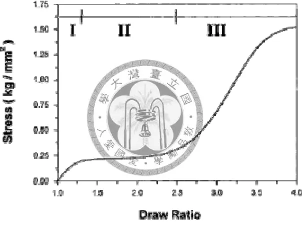
There are many papers showing the evidences of the structural changes during drawing and spinning processes. The behavior of stress-draw ratio curve of the melt-quenched amorphous PTT film during uniaxial drawing could be divided to there regions, including initial(I), plateau(II), and final(III) [18, 19].(Figure 1.1) A further increase of the draw ratio above 2.5 causes a significant strain hardening as shown in region III. The fast increase of the modulus in this region indicates that there might be major structural changes occurring in addition to the orientation of the chain along the

(29)

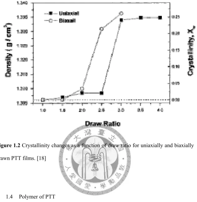
deformation direction. Simultaneously, the crystallinity (measured by density) of the PTT abruptly rise at draw ratio 2.5. (Figure 1.2) On the other hand, the oriented structure development is observed by orientation factor (the definition of which can be found in 2.8.3 orientation factor). Orientation factor of the melt-quenched amorphous PTT film, calculated by IR dichrocic ratio of characteristic bands (by equation 2.18), increase with increasing draw ratio[16]. Similarly, Orientation factor of partial oriented yarns (POY) PTT fiber, which is calculated by intensity of WXRD (by equation 2.19), increase with increasing draw ratio and take-up speed[20]. Moreover, the birefringence of PTT increase with spinning speeds. Besides, the conformation of PTT chain change during drawing or spinning process (which will be discussed in 1.5 The transition of conformation during crystallization).

In order to further understand the molecular mechanical mechanism of stress-induced crystallization, some theoretical works using molecular simulation have been conducted recently. Linear polyethylene (PE) is used in most of simulations. The crystallization from an oriented amorphous state has been reported by Koyama[21] in 2002. The crystallization, spending around 30 ns simulation time, is evidenced by the increase of mean length of the trans sequences, and the increase order in the pre-oriented direction. Furthermore, the temperature effect and non-isothermal extensive process are considered by Lavine [22] in 2003. The orientation factor increase with draw ratio until high extension, and the number of crystals, crystal size, and the angle that the crystal c-axis align along the stress direction, increase as the annealing temperature increases. In non-isothermal extensional process, the crystallization is observed to show the rapid densification corresponding to increasing order parameter between 360K and 320K (around Tm). He also proposed that the mechanism of oriented

(30)

crystallization can be interpreted as competition between the rate of the relaxation of deformation-induced orientation and the rate of the nucleation which locks in structure at some level of orientation. Moreover, the extensional flow process inducing the shish-kebab crystallization has been reported by Dukovski[23] in 2003, and the secondary nucleation process by creating a knot in the polymer system has been studied by Saitta[24] in 2002.

Figure 1.1 Stress-draw ratio curve of melt-quenched amorphous PTT film during uniaxial drawing around Tg. [18]

(31)

Figure 1.2 Crystallinity changes as a function of draw ratio for uniaxially and biaxially drawn PTT films. [18]

1.4 Polymer of PTT

Poly (Trimethylene Terephthalate) (PTT), such as Poly( Ethylene Terephthalate) (PET) and Poly(Buthylene Terephthalate) (PBT), is a member of aromatic polyester polymers. (Figure 1.3) PTT is synthesized by the condensation of 1,3-propanediol (PDO) with either terephthalic acid or dimethyl terephthalic. Recently, breakthroughs in raw material, PDO, synthesis reduce the cost of PTT, and offer a chance to catch up with its homologues neighbors PET and PBT in the commercial material markets.

(32)

1

2 3

4

5 6

1

2 3

4

5 6

Figure 1.3 Chemical structure of a repeating unit of PTT (a) and a fragment (4 repeating units) of the PTT chain (b). Carbon atoms are shown in grey, oxygen in red, and hydrogen in yellow. The green cylinders connecting the centers of adjacent aromatic rings are taken as elementary segments in the precursor analysis.

The crystal structure, mechanical properties, and thermal properties of PTT have been reported experimentally. PTT is a triclinic crystalline structure which contains two chemical repeat in each cell, with the cell parameters reported in Table 3.1. The purely crystalline density is 1.387~1.43 g/cc[25-27] by theoretical calculations; the experimental density of semicrystalline is reported to be 1.31~1.35g/cc [16, 28]; the simulation result is reported to be 1.262 g/cc[29]. In PTT crystal structure, three methylene units exhibit very compliant gauche-gauche conformation resulting in its outstanding elastic recovery and resiliency compared to PBT and PET. Experimental measurement of Young’s modulus is reported to be 2.3~2.8GPa[30-32]; the simulation results were reported to be 3.84±0.16 GPa in amorphous system[29] , and 6.31±0.64

a)

b)

(33)

GPa in semicrystalline system[33]. Besides, the experimental result of the melting point is reported to be 499~503K[34-36], and the equilibrium melting temperature Tmo is estimated to be 510~525K[37, 38] by linear Hoffman-Weeks extrapolation (LHW), and 546~578K[38] by non-linear Hoffman-Weeks extrapolation (NLHW). The glass transition temperature is reported to be 315~348K.[30, 35]

The crystallization behaviors of PTT have been studied by isothermal (melt and quench) crystallization and non-isothermal crystallization process. In isothermal process, Avarmi model is the most popular theory for analysis of the crystallization rate from experiment:

X

( )

t =1−exp(−K_Atⁿ^A) (1.1a)

ln

{

−ln

[

1−^X

( )

^t

] }

=ln

( )

^KA +ⁿAln

( )

^t (1.1b)

where X(t) is normalized crystallinity at time t, k is crystallization rate constant, and nA

is Avrami exponent. (See Table 1.1) From the data fitting by the equation (1.1b), the crystallization behavior can be identified as primary crystallization, which consists of an outward growth of lamellar stacks until impingement, and a secondary crystallization of filling in the spherulities of interstices[36]. Some results suggest that both primary and secondary crystallizations overlap[36], but others consider the secondary crystallization occurs after primary process completes[39]. The Avrami exponent, n, have been reported with different temperature region shown in Table 1.2. Based on the nA value, we know that the mechanism of the primary crystallization are an athermal nucleation with two-dimensional crystallization growth (nA=2) above Tg, and three-dimensional

(34)

crystallization growth (nA=3) around Tm. The high nA value (nA=5) indicates a solid sheaf growth with athermal nucleation in cold crystallization about Tg. On the other hand, except Avarmi model[40, 41], a modified Avarmi model[42], Ozawa model[41, 42] , and Ziabicki model[42] have been used to analyze the crystallization rate in non-isothermal crystallization, respectively.

Modified Avarmi model

X

( )

t =1−exp

[ (

−KAt

)

ⁿ^A

]

(1.2)

where KA is crystallization rate, which the units are given as inverse of time,

Ozawa model

( )

⎥⎥

⎦

⎤

⎢⎢

⎣

⎡

⎟⎟⎠

⎜⎜ ⎞

⎝

⎛

− φ

−

=

nO

KO

exp 1 T

X (1.3)

where X(T) is normalized crystallinity at temperature T, KO is crystallization rate, and φ is cooling rate,

Ziabicki model

( )

K

( )

T

[

X

( )

t

]

dt t dX

Z −

= 1 (1.4)

(35)

( ) ( )

⎥⎥

⎦

⎤

⎢⎢

⎣

⎡ −

−

= _,_maxexp 4ln2 ₂^max ² D

T K T

T

K_Z _Z (1.5)

where Tmax is the temperature at which the crystallization rate is maximum, KZ,max is crystallization at Tmax, D is the width at half-height determined from the function of crystallization rate, and is also proposed the kinetic crystallization ability of the semi-crystalline polymer

G ^m K

( )

T dT K D

g

T

T max

5 . 0

2 ln 2 1

0

⎟⎠

⎜ ⎞

⎝

= ⎛

=∫ ^π ^(1.6a)

φ

G_c = G (1.6b)

The exponent of Avarmi and Ozawa model summarizes in Table 1.3, and the results of Ziabicki model in Table 1.4ab. From Avarmi model, the nA value decrease with increasing cooling rate (from 4 to 3), which indicated the nucleation mechanism transition from a thermal to an athermal model. [36] From modified Avarmi model, the nA value was reported to be a constant[42]. Besides, the Tmax value decrease with increasing cooling rate, and D value increase with increasing cooling rate[43, 44]. These analysis results conclude that the crystallization rate increases with increasing cooling rate.

(36)

Table 1.2 Summary of Avrami exponent in isothermal process.

Temperature region Avrami exponent, n Reference Primary crystallization

328~348K(cold crystallization) ~5 [36]

443~485K 2~3 [36]

448~468K 2.6~3.8 [45]

450~480K 2.5~3 [39]

453~475K ~2 [40]

475~503K 2.7~2.84 [34]

Secondary crystallization

450~480K ~1 [39]

Table 1.3 Summary of model’s exponent in non-isothermal process.

Cooling rate Exponent Reference

Avrami model

0.63~ 20K/min 1.9~3.7 [40]

5~25K/min 4 ~ 3.3 [41]

modified Avarmi model

5~30K/min 4.4~4.7 [42]

Ozawa model

0.63~ 20K/min 1.9~3.7 [40]

5~25K/min -- [41]

5~30K/min 2.4~4.37 [42]

(37)

Table 1.4a The kinetic crystallizability of non-isothermal process analysis by Ziabicki model[44].

φ (K/min) D Kmax Gc

5 7.6 0.75 1.21

10 8.2 1.12 0.98

20 8.9 1.94 0.92

30 9.3 3.24 1.13

40 10.6 3.58 1.01

average 1.05

Table 1.4b The kinetic crystallizability of non-isothermal process analysis by Ziabicki model[43].

φ (K/min) Tmax(^oC) D X&max(x10²) Gc

5 185.82 9.84 1.05 1.31

10 178.63 11.52 1.91 1.41

15 173.45 19.66 2.23 1.86

20 170.27 18.37 2.99 1.75

30 163.90 20.36 3.26 1.41

40 158.53 24.99 3.67 1.46

50 152.33 28.46 3.63 1.32

average 1.50

(38)

1.5 The transition of conformation during crystallization

The drawing process which would rapidly enhance the crystallization by ordering the polymer segments have been introduced in the previous section. Many researchers are interested in changing the conformation of PTT polymer during the drawing or spinning process. In particular, they focus on the torsion angles of the propylene glycol segments (O-CH2-CH2-CH2-O). The crystal lattice of the PTT has been studied by Desborough[26] and Poulindandurand [25]. They both reported that the distribution of the torsion angle of the O-CH2-CH2-CH2-O segment is tans-gauche-gauche-trans (t-g-g-t) in the crystalline state. However, what the torsion angle distribution in amorphous state is and how they transfer form amorphous to crystalline state remain unclear.

Many papers were reported trying to answer above questions, but the results were not very consistent. Base on PoulinDandurand’ theoretic work [25], Kim [16] calculated the energy level of each conformation state and proposed that the g-t-t-g conformation is much more populous in the amorphous region than t-t-t-t is. In contrast, Ohtaki[46]

argued that the conformation is random in amorphous state. Jeong[19] reported the content of the gauche state of φ2 (See Figure 1.3) to be 33.4% in fully amorphous state, which is estimated by the ratio of the infrared intensity of the gauche and trans conformer.

The mechanism of the conformation transition from amorphous to crystal phase has also been studied using IR spectroscopy, X-ray scatting, and ¹³C solid-state NMR.

From IR spectroscopy, which is the most popular method, some bands have been

(39)

identified to reflect the torsional state of propylene glycol segments during crystallization process. However, we found that the bands corresponding in phase and conformer are not very consistence from researchers’ identifications, although the assignment for each band agreed with each other. We summarize those bands and their relation with phase and conformer in Table 1.5. By comparing the IR spectroscopy of the pure crystalline phase and amorphous phase, Kim’s group reported that the transition of the torsion angle is form gttg to tggt [16] during cold-crystallization. This process almost stops below 80^oC.[17] Murase’s group reported similar results in which the φ2 conformation is form tt to gg when the polymer is subjected to a long annealing time[46]. On the other hand, the conformational dynamics was investigated during drawing process. Chuah’ group[28], Kim’s group[17], Jeong[19], and Murase’s group[46] all reported that the φ2 conformation is form tt to gg accompanying the draw ratio. Further, Chuah and Jeong both proposed the linear relationship between the gauche content of φ2 and crystallinity during stress-induced crystallization. Besides, Chuah’s group[47] reported the fiber conformation changes from tggt to tttt at high drawing speeds and some specific temperature by using X-ray scatting to observe the unit cell length of the crystal structure. Murase’s group[48] reported the conformation which only focus on φ1, however, changes from trans to gauche in half and remains in other half during drawing process by using ¹³C NMR technique.

Above all, in crystal state, the φ2 conformation exists largely in the gauche state, and the φ1 conformation exists largely in the trans state; in amorphous state, the φ2

conformation exists mostly in the trans state, but the φ1 conformation is unclear.

Moreover, the transition during annealing process, the φ2 conformation changes form trans state to gauche state but φ1 conformation is unclear; the transition during drawing

(40)

process, the φ2 conformation changes form trans state to gauche state, if polymer chains undergo sufficient thermal relaxation; however, the φ1 conformation is unclear.

Table 1.5 The identification of IR bands corresponding with propylene glycol segments.

Band Assignment Phase Conformer type

811 CH2 rocking[28, 49] amorphous[19, 28] trans [19, 28]

933 CH2 rocking[28, 49, 50] crystal[16, 19, 28]

Amorphous[50] gauche [19, 28]

1037 CC stretch[16, 28, 46] Amorphous[16]

Crystal[28, 46] gauche[16, 46]

1043 CC stretch[16, 49, 50] crystal[16, 49, 50] gauche [16] [49]]

1358 CH2 wagging [16-18, 28, 46, 49, 50]

Crystal [16-19, 28, 46, 49, 50]

trans [18]

gauche [28, 46]

1385 CH2 wagging [17, 18, 28, 46, 49, 50]

crystal[49, 50]

amorphous[17, 18, 28, 46]

gauche [18]

trans [28, 46]

1471 CH banding[16, 17, 49, 50]

crystal[16, 17, 19, 49, 50]

amorphous[16]

1.6 Motivation

While experimental and theoretical efforts are made to verify and explain the molecular mechanism in the growth of nuclei in polymeric materials, the primary stage of polymer crystallization is less well understood. In experiment, the crystallization of the polymer has been studied by isothermal, non-isothermal, and stress-induced processes, and establishes the knowledge of the kinetics behaviors, the phenomena of the early ordering structure, and orientation crystallization behaviors. The molecular mechanism of the crystallization, however, seems difficulty to study experimentally. On

(41)

linear polymer (PE). Furthermore, in order to reduce the simulation time, coarse-grained or bead-spring models are used. Such models overlook the atomistic details of the polymers so that detailed change in chain conformation could not be observed. It could potentially lead to discrepancies found between in some properties between simulations and experiment.

In this work, we use fully atomistic models to simulation the crystallization process of poly(trimethylene terephthalate), PTT. Unlike coarse-grained or bead-spring models that are more often adopted in simulation for crystallization process of polymers[12-15, 51], atomistic molecular models, while more computational demanding, provide a much better resolution on the detailed packing structure. Our simulations focus on the ordering of structures (nuclei precursors) appearing in the isothermal and stress-induced crystallization process. We study the temperature dependence of the amount of such clusters, the behavior of ordered structures and torsion angle transition during drawing and annealing processes, and try to understand the mechanism of the nucleation at the early stage of crystallization.

(42)

2 Theory

2.1 Molecular dynamic simulation

Recently, computer simulations have come to be recognized as a powerful and promising tool to investigate the molecular process of polymer crystallization. A polymeric system contains a large number of atoms, and the motion of atoms exist large degrees of freedom. The large degrees of freedom increase the difficulty to understand the relationship between the properties and motion of atoms. Some simplified polymer models have been proposed to describe the general behaviors of polymer. Now, more realistic models can be considered because of the significant advancement in the computation power.

Among of all simulation methods, molecular dynamic simulation is the most popular technique for computing the equilibrium and dynamic properties. The method is solution of classical equations of motion, which are integrated numerically to give the information on the positions and velocities of the atoms in the system. The net forces on each atom are calculated by the differentiation of the potential energy.

2.2 Algorithm

There are some algorithms used in the molecular dynamics simulation to solve for the equations of motion. In this work, Verlet method is used in all simulation. The initial form of the Verlet equations is obtained by utilizing a Taylor expansion of the position at time t + Δt and t - Δt

(43)

( ) ( ) ( ) ( )

²

( )

³

( )

⁴

! 3 1

! 2

1 t r t t o t

m t t f

t t r t t

r _i

i i i

i

i +Δ = + Δ + Δ + &v&& Δ + Δ v v

v

v ν (2.1)

( ) ( ) ( ) ( )

²

( )

³

( )

⁴

! 3 1

! 2

1 t r t t o t

m t t f

t t r t t

r _i

i i i

i

i −Δ = − Δ + v Δ − &v&& Δ + Δ v

v

v ν (2.2)

where )fv_i(t

is the net force applying on the i atom at time t, m is the mass of the i _i atom. Summing the two equations gives

( )

²

( ) ( ) ( )

^t² ^o

( )

^t⁴

m t t f t r t r t t r

i i i

i

i +Δ = − −Δ + Δ + Δ

v v v

v (2.3)

and subtracting the two equations gives

( ) ( ) ( ) ( )

²

2 o t

t t t r t t

t rⁱ ⁱ

i + Δ

Δ Δ

−

− Δ

= v + v

νv (2.4)

Above can give the position (equation. 2.3) and velocity (equation. 2.4) of each atom at each simulation time.

2.3 Force field

Forces resulting from atomic interactions are in the above algorithm. The concept of calculation is

(44)

2 2 ( ) )

) ( (

dt t r m d t r f

t

U _i

i i

i

v v

v = =

∂

−∂ (2.5)

where U(t) is the overall potential energy at time t. The potential energy is the summation of the valence types (band, angle, torsion, and inversion energy) and non-bond types (coulomb and van der waals interaction). In this work, we chose Dreiding[52] force field whose general forms are described below.

2.3.1 Bond energy

The bond energy is described by harmonic style as following

2 0) 2 (

1K R R

U_b = _b − (2.6)

where Kb is constant, and R0 is equilibrium length of bond. The parameters of the bond stretch are shown in Table A.2.

2.3.2 Angle energy

The angle energy is described by cosine harmonic style as following

2 0) cos 2 (cos

1 _θ θ θ

θ = K −

U (2.7)