灰色理論結合強化樣本技術應用於營建公司破產幾率預測之研究

(1)

國立臺灣大學工學院土木工程學系碩士論文

Department of Civil Engineering College of Engineering

National Taiwan University

Master Thesis

灰色理論結合強化樣本技術應用於營建公司破產幾率預測之研究

Predicting default probability in construction industry basing on Over-Sampling Technique for

Grey SystemTheory

張克戰

Truong Khac Chien

指導教授：曾惠斌教授 Advisor: Prof. Tserng, Hui-Ping

中華民國103年6月

June, 2014

(2)

ACKNOWLEDGEMENT

This paper could not have been completed without the help, encouragement and support from a number of people who all deserve my sincerest gratitude and appreciation.

First of all, I would like to thank Prof. Tserng, Hui-Ping, my supervisor. I’m indebted to his inspiration, scholarly supervision and intellectual support throughout the course of writing this graduation paper. His continual encouragement, careful reading, critical comments and patient guidance made my work more enjoyable and easier.

Next, I owe sincere and earnest thankfulness to professors and staff members of not only Civil Engineering Department, National Taiwan University but also National University of Civil Engineering in Vietnam, for their supports during my study. Special thank is due to many graduates I have worked with, especially Po-Cheng Chen for his suggestion, assistance to complete my thesis. It is my pleasure to thank those who made the research possible.

I would also like to show my gratitude to my wife, Nguyen Thi Lien, for her love, encouragement, spiritual supports through the years. This dissertation would not have been possible without her supports.

Last but not least, I am truly indebted and thankful to my parents and my older brother. Their unconditional support, love, patience and understanding bring me overcome the challengers.

(3)

ii ABSTRACT

Bankruptcy Prediction has been a hotly-debated topic among many people in business area. The fact is that once the firm goes bankrupt, it will be disastrous to not only firm itself but also other stakeholders. Many available methods have been applied to predict the possibility of business collapse; almost all of them were based on financial ratio analysis. Grey System Theory, used in the previous thesis for predicting default probability of construction firms, has brought some feasible results, by relying on the 19 initial financial ratios.

This study, with the aim of enhancing the Grey Theory application, employs Over-sampling technique before applying Grey System Theory. The results of this study are then compared with those of the prior research. Furthermore, replication and Synthetic Minority Over-sampling Technique (SMOTE), two over-sampling techniques are proposed to resolve the imbalance problem in data set.

The results reveal that over-sampling techniques could improve the predicting performance of Grey System theory. Additionally, between these two kinds of over- sampling techniques, SMOTE surpasses Replication in terms of prediction capability.

Key words: Over-sampling, SMOTE, Grey System Theory, Synthetic Degree Incidences, financial ratio, ROC curve, construction industry.

(4)

iii

LIST OF FIGURES

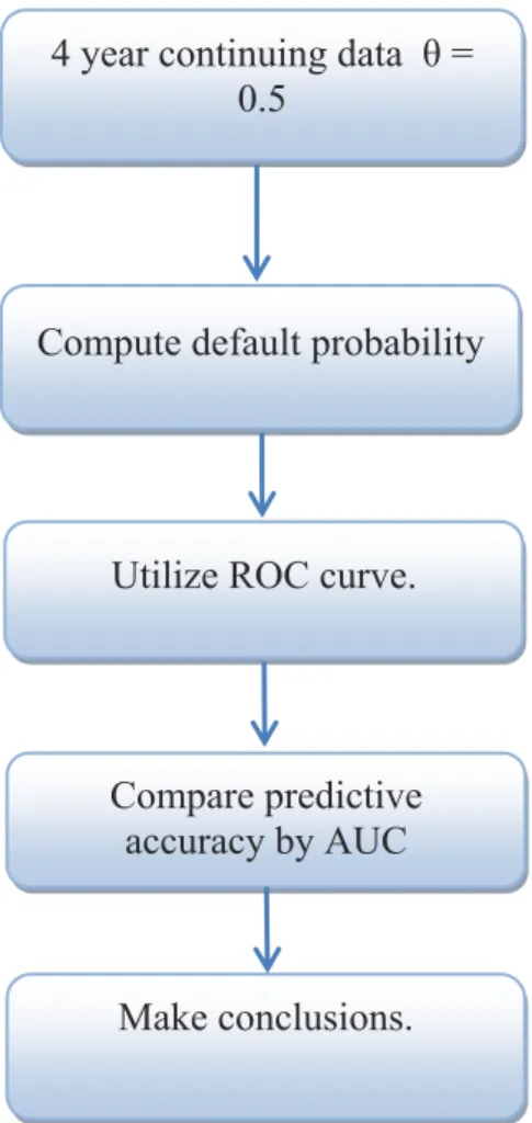
Fig.1.1The produce of research...5

Fig.3.1 An example of ROC curve...32

Fig.3.2 Schematic of a ROC………...………...…………...…….33

Fig.4.1 The algorithm chart of the data analysis process...45

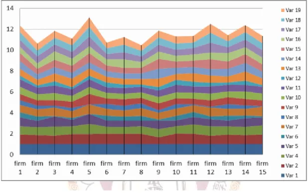
Fig.5.1 Sum of the synthetic degree calculated based on matrix ρ...…...…..56

(8)

vii

LIST OF TABLES

Table 3.1 Types of error of ROC………....………....………...………..31

Table 4.1 Information of the defaulted companies …………...….……….…...….36

Table 4.2 Selected ratios’ classification … ………....………...….38

Table 4.3 Definition and usage ratios ………....…….………39

Table 5.1 Selected variables and their default probability correlation……..……..…....46

Table 5.2 5 year history data of firm No.1 ……….…………...…...47

Table 5.3 The absolute j value of firm No.1……….…………...…...49

Table5.4 The initial images value of firm No.1………...….…………...51

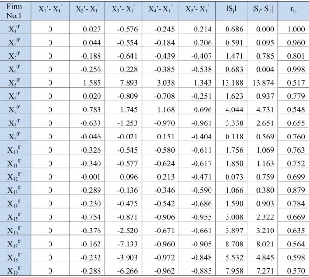
Table 5.5 The relative rj value of firm No.1………...…………52

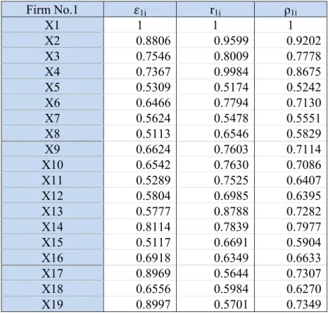
Table 5.6 The synthetic ρj value of firm No.1……….…………....53

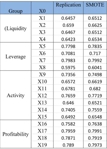
Table 5.7 AUC value (846 samples, = 0.5, 4 years, .) ……….………...60

Table 5.8 AUC value (846 samples, = 0.5, 19 initial var) ………...….…..…62

(9)

1

CHAPTER 1: INTRODUCTION

1.1

Background

Bankruptcy Prediction has inherently been a common topic in business area. The economic crisis over the last few years has made this topic more urgent than ever before.

A business is declared bankrupt when it is unable to pay off its debts. Once the firm goes bankrupt, it will cause intense damages to both the firm itself and its shareholders alike.

No parts of business are immune to bankruptcy. Bankruptcy can happen in any aspects of business, ranging from monetary industries such as banking, financial institutions to non-related monetary sectors such as manufacture, construction and so on.

However, almost all previous studies touching bankruptcy prediction overlook the specific area; they solely focus on general business area.

The construction industry indeed plays an important role in enhancing the economic performance and the national welfare of a country by transforming various resources to construct economic and social facilities (Basir, 2000). The construction project is usually a prolonged and a costly process. Construction enterprises, due to high competitiveness, have to reluctantly reduce their profit to win the bid, which exposes them to the default risk. Besides, the cycle of construction projects are relatively long, so the income of the construction firms might be easily affected by the price changes in materials, manpower, machine’s expenditure, as well as the adjustment of legislation and policies. Therefore, regular evaluation of financial performance should be priority of construction firms so that they are able to detect any potential company failures at the earliest opportunity, from which timely and appropriate strategies can be put in place to help them to recover. The early warning of construction contractor failure is an

(10)

2 important issue for government organizations, construction owners lending institutions, surety underwriters, and contractors (Tsai et al., 2011).

1.2 Motivation and Problem statements

The construction industry always plays a crucial role in a country’s economic flourish. It is the cornerstone and connecting factor of the other industries. However, the contractors are confronting with lots of difficulties in an increasingly competitive environment nowadays. The past data collected from the U.S. market indicated that the failure rate among construction firms has reached a critical level (Kangari et al 1992;

Ekanayake 2008). Meanwhile, some highlighted characteristics of the construction industry and construction project such as unique, long term investment, big invested capital, etc. make the financial characteristics of construction industry different from those of other industries.

A lot of models anticipating business malfunction have been proposed.(e.g.

Bevear, 1966; Altman, 1968; Ohlson, 1980; Shin, 2001; Chen 2004; Chien, 2005).

Nevertheless, most of available researches focus on default prediction of business in banking and finance sectors; quite few researches work on the default probability prediction of construction firms.

Earlier statistical models focused on anticipating bankruptcy utilizing statistical discrimination methods. For example, Beaver (1966) studied univariate discrimination models. His model emphasized individual signals of impending matters without revealing the interaction of variables. Altman (1968) established a popular multivariate prediction framework known as the Z- score model. Then, 1977, Altman et al, developed a more comprehensive discriminant model, the Zeta model. Ohlson (1980) used the maximum likelihood estimation of conditional logit model in developing the

(11)

3 capacity of bankruptcy prediction. Despite some significant contributions, the aforementioned researches have a number of limitations: Firstly, they only used financial ratios did not consider other factors such as economy, operation, and management; therefore, did not meet the total relationship between the causes and effects of business failure. Secondly, static models ignore the time –series effects of a firm’s financial and operational performances on the risk of business bankruptcy. Lastly, these models just looked at industries in general; less attention was paid to construction industry.

In conclusion, understanding the mechanism of failure is a surefire way to business breakdown avoidance. Furthermore, little attention has been given to predicting the probability of construction company failure. Due to the high risk default probability of construction industry and its different characteristics from others’; there should be study to predict default probability of the construction contractors.

The previous thesis of Le Quyen showed some fairly accurate results in the application of Grey System Theory on the default probability of the construction firms. However, some shortcomings were inevitable. The number of non-defaulted samples greatly exceeds the defaulted samples. Consequently, to tackle imbalance data problem, in this research, two different over-sampled approaches namely Enforced Training and Synthetic Minority Over-Sampling Technique were used.

1.3 Research objectives

Apply the Grey system theory for analyzing the impact of financial ratios on the default probability of the construction firms.

(12)

4 Apply over-sampling technique before using Grey System to resolve imbalance data problem (the number of non-defaulted samples greatly exceeded the number of defaulted samples). The present research aims to achieve two principal objectives:

1) Compare with previous research which method gives higher efficiency.

Give the result that: whether Grey system Theory has the imbalance problem or not.

2) Enhance the usefulness of Grey Theory

1.4

Research scope and limitations

This research only used financial ratios. Other factors such as economy, operation, and management were not considered in this study; therefore, the total relationship between the causes and effects of business failure was not met.

The data used in this thesis are obtained from US stock market in the period of 1970-2006, and concentrate on construction firms which have different characteristics from other industries’. Therefore, this study only concentrates on construction contractor. It means that the results should be cross-checked in data of other industries.

Additionally, the accuracy of any financial ratio-based predictive model largely depends on the reliability of accounting data source. In some real cases, financial data might be manipulated, which leads to failure of model. Besides, the data used in this research are all available data firm years and the bankrupt sample is the data from the last financial statement issued before the firms declared bankruptcy. That is, this model is not able to assure for predicting insolvency more than one year prior to bankruptcy.

(13)

1.5 T

The

fram

and t

mode the p

Thesis str

remainder

Figure 1 mework of th

Chapter thesis struct

Chapter els which ap present resea

ructure

of this resea

1-1 shows hesis is divid

1: Introduc ture.

2: Review pplied for n arch.

arch is orga

Figure 1.1

procedure ded in five c

ce the back

w the litera non-construc

Conclu Co Data Col Stud

L

anized as fol

: The prod

of this res chapters as

kground, m

ature, regar ction and co usion and S ompare the M

Data Analy llection and dy of Metho Literature Re

Topic Selec llow:

duce of rese

search. Bas follows:

motivation, p

rd to the p onstruction Suggestions

Models ysis

Arrangeme odologies

eview ction

earch

se on the a

purposes an

previous de companies ent

above steps

nd contribu

efault predi and related

5 s, the

utions,

iction d with

(14)

6 Chapter 3: Introduce the methodologies of default prediction, Grey System Theory, how to apply Over-sampling technique to resolve imbalance data problem, and how to use ROC curve (Receiver Operating Characteristic curve) to evaluate the prediction power of this model.

Chapter 4: Presents the standard of data collection.

Chapter 5: Analyzing and validating input data.

Chapter 6: Present the conclusions and suggestions.

(15)

7

CHAPTER 2: LITERATURE

This chapter presents a brief overview of the development of bankruptcy prediction model in both general industry and construction industry.

2.1 Default prediction researches

There have existed numerous approaches to the corporate failure prediction in general business area so far. Beaver was the first scholar using financial ratio in predicting bankruptcy. After Beaver, a lot of other researchers employed different methods such as multivariate discriminant analysis (Altman, 1968), logit (Ohlson, 1980) or probit (Zmijewski, 1984). These models were then developed in accordance with the information form financial statements to evaluate strengths and shortcomings of a company’s financial status.

The application of financial ratio models to determine a business’ profitability, and hence chances of its survival, attracted many researchers’ concern in both general business (Altman, 1967; Beaver, 1968; Taffler, 1983; Robertson (1984); Keasey and Watson, 1986) and the construction domain alike (Mason and Harris, 1979; Kangari, 1988; Abidali, 1990; Russell and Jaselski, 1992; Langford et al., 1993; Ramsey Dawber, 1993)

1. Fitz Patrick (1932)

The first author to use financial ratio model was Fitz Patrick (Fitz Patrick, 1932).

He studied 19 bankrupt firms and 19 non-bankrupt ones. The research found 3 years before bankruptcy, the financial ratios were significantly changed.

(16)

8 2. Beaver (1967)

William H. Beaver is one of the first developers of business failure prediction using quantitative method. The methodology adopted by him is discriminate analysis (DA). He collected data from Moody’s Industrial Manual – 79 firms that collapsed during 1954 to 1964. None of these companies was construction firm; they mostly were in manufacturing sector. Non-defaulted firms in the same industry and asset size were also assembled to distinguish and discriminate against the distressed firm.

There were 30 ratios commonly used in the financial literature in Beaver’s study.

His research aims to discover the capability of these ratios to differentiate the bankrupted group from the non-bankrupted one. In his study, various methods such as mean values, mean asset size, dichotomous classification tests and analysis of likelihood ratios were integrated to analyze the ratios. After finalizing the calculated process of these ratios for the period of 5 years prior to bankrupt, the result of Beaver’s study indicated that the cash flow – total debt ratio was the overall best predictor. Another contributor of his research was the affirmation of using accounting data in the forecast of business bankrupt. What could be drawn from his study was that using financial ratio could give the early warning of 5 years before bankruptcy.

3. Altman (1968)

Beaver’s research has certain values when pointing out the importance of using financial ratio in predicting default; however the discriminatory power of the independent ratio makes this research not a perfect one. To address this drawback, E.Altman (1968) developed Beaver’s method and established an innovative model named mutlti-variate approach. In this research, Altman also reconfirmed the principal role of using financial ratios as a predictor of corporate. Altman used 33 failed

(17)

9 manufacturing firms matching up with the same number of non-failed firms in the period of 1946 to 1965. The criteria of matching were the same industry and roughly similarity in asset size. Using the Multiple Discriminant Analysis (MDA) technique in the study, the 22 financial ratios served as input variables to analyze. The stepwise method then applied to choose an optimal combination of five variables from the 22 ratios initially selected. Finally, Altman’s model proposed a following linear function using five variables

Z = 1.2X1+ 1.4X2 +3.3X3+ 0.6X4 +1.0X5 (1) Whereas:

X1: Working Capital/Total Assets

X2: Retained Earnings since Inception/Total Assets X3: Earnings before Taxes and Interest/Total Assets X4: Market Value of Equity/Book Value of Total Debt X5: Turnover/Total Assets.

Accordingly, businesses were classified as follows:

 Z - score less than 1.8 implied certainty of imminent failure;

 Z - score between 1.8 and 2.7 revealed the “zone of ignorance” or ‘grey area’ , where companies were deemed to be at risk; and

 Z - score greater than 2.7 (initially 2.9), indicated a potential for long term solvency.

The model correctly classified 95 percent of the total 66 sample firms (correctly classifying 94 percent as bankrupt firms and 97 percent as non-bankrupt firms) one-year prior to bankruptcy. The percentage of the accuracy fell down with increasing number of years before bankruptcy. This technique has a strong reputation in the history of

(18)

10 corporate bankruptcy models until the 1980s and is weidely applied as the baseline for comparative studies.

4. Ohlson (1980)

Ohlson (198) is another researcher using financial ration as predictors of bankruptcy to develop his bankruptcy prediction model. His research analyzed nine financial ratios of firms’ size, leverage, liquidity and performance, using logistic regression. Data were gathered from 1970 to 19976 and included 105 defaulted and 2,058 non-defaulted industrial enterprises. His model’s kernel function was built as follows:

Probability of defa

ult 1 1

1

z

z z

e

e e^

 

 

Z = -1.3-0.4X1 + 6.0X2 – 1.4X3 + 0.1X4 – 2.4X5 -1.8X6 + 0.3X7 – 1.7X8 -0.5X9

Where:

X1= Log (Total Assets / GNP Price-level Index) X2 = Total Liabilities / Total Assets

X3 = Working Capital / Total Assets X4 = Current Liabilities / Current Assets

X5 =1 if total liabilities exceed total assets, o if otherwise X6 = Net Income / Total Assets

X7 = Funds provided by Operation / Total Liabilities

X8 = 1 if net income was negative for the last two years, 0 if otherwise

(19)

11 X9 = Measure of Change in Net Income

5. Taffler (1983)

In the UK, another two authors Taffler and Tishaw (1977) adopted a similar methodology as other seniors’, basing on a sample of 92 manufacturing companies. The resulting Z score equation was based on a combination of four categories ratios;

however, undisclosed coefficients:

Z = c0 + c1X1 + c2X2 + c3X3 + c4X4 (2) Where:

X1: Profit before Tax/Current Assets (53%) X2: Current Assets / Current Liabilities (13%) X3: Current Liabilities/Total Assets (18%) X4: No Credit Interval (16%)

The percentages give guidance to the relative weightings of the ratios. Taffler and Tishaw declared a 99% successful classification based on the original 92 companies from which the model was conducted. However, this success assurance lost its value when the model was re-tested by Taffler (1983) with a sample includes 825 companies.

The two models were developed by Altman and Taffler both bolstered the significance of the ratio variable of turnover to total assets as a positive indicant that contributed to corporate bankruptcy.

6. Robertson (1984)

In an effort to address the question of a theory on corporate failure, Robertson (1984) developed a ratio model that worked with general applicability to all industries.

He declared that there were a priori determinants of corporate failure from their financial ratios. Robertson suggested ratios expressing trading stability, declining profits, declining working capital and increases in borrowing as predictive

(20)

12 characteristics. Instead of the simple turnover to total assets utilized by Altman (1983) and Taffler (1983); Robertson (1984) utilized the ratio of turnover less total assets to turnover, to display the importance of trading stability in his model. The outcome model combined five ratio variables were presented as Equation 3:

Z = 0.3X1+ 3.0X2 +0.6X3+ 0.3X4 +0.3X5 (3) Whereas:

X1: (Turnover – Total Assets)/Turnover;

X2: Profit before Tax/Total Assets;

X3: (Current Assets – Total Debt)/Current Liabilities;

X4= (Equity – Total Borrowings)/Total Debt; and X5= (Liquid Assets – Bank Overdraft)/Creditors.

2.2 Default prediction researches in construction industry

According to S. Thomas NG, “Pertinent forecasting techniques for construction company failures include the (1) ratio analysis; (2) multiple discriminant analysis; (3) conditional probability models; and (4) subjective assessment”. In completing the present study, the author read several relevant studies in the construction industry as follow:

1. Mason and Harris (1979)

Mason and Harris (1979) developed a six-variable model to assess construction organizations in UK. In this study, a sample of 20 bankruptcy and 20 non- bankruptcy firms was selected. Basing on the MDA), the discriminant function was developed as below equation. A positive Z-score indicated a long-term solvency, while a negative value was classified as a potential failure. Their model was conducted with a multiple regression approach and presented as:

(21)

13 Z =25.4 – 51.2X1+ 87.8X2 – 4.8X3 – 14.5X4– 9.1X5 – 4.5X6 (4) Where:

X1: Profit Before Tax and Interest/Opening Balance Sheet Net Assets;

X2: Profit before Tax/Opening Balance Sheet Net Capital Employed;

X3: Debtors/Creditors;

X4: Current liabilities/Current assets;

X5:Log10 (days debtors); and X6: Creditors Trend Measurement.

While a positive Z-score indicated a long-term solvency, a negative value revealed a potential bankruptcy. The variable profit before tax and interest to opening balance sheet net assets (X1) was indicated as a negative sign in the research. This implies that a higher value of a return on net assets produces a greater tendency for bankruptcy, which is rather unconvincing.

2. Abidali, 1990

Abidali also developed a Z-score model used in vetting construction companies on the tender lists. Using multivariate discriminant analysis to produce a predictive model including seven variables, 31 different variables were initially adopted. The best discriminating variable is selected according to Wilks Lambda criteria. The Z-score model is shown below in following equation:

Z =14.6 + 82.0X1 – 14.5X2 +2.5X3 – 1.2X4 + 3.55X5 – 3.55X6 – 3.0X7 (5)

Where:

X1 =Profit after Tax and Interest/Net Capital Employed;

X2 = Current Assets /Net Assets;

(22)

14 X3 =Turnover/Net Assets;

X4 =Short Term Loans/Profit before Tax and Interest;

X5 =Tax Trend over three years;

X6 =Profit after Tax Trend over three years; and X7 =Short Term Loan Trend over three years.

3. Russel (1988) and Jaselskis (1992)

While some previous researchers only focused on analyzing financial variables, Russell and Skibniewski (1988) deepened their research by presenting all the factors involved in the construction contractor prequalification decision-making process, which are closely related to contractor default risk. Beside financial soundness, management capability, and economic condition as well as technical expertise are also essential factors to construction contractors’ success. Their research model was introduced with 5 variables, cooperating 4 financial ratios and one management related variable:

Y = 2.27 – 7.72 X1 + 45.05 X2 + 13.94 X3 - 13,24 X4 – 34.42 X5 (6) Where:

X1: Cost Monitoring (not performed = 0; performed = 1);

X2: Under-Billings to Sales;

X3: Total Current Liabilities to Sales;

X4: Retained Earnings to Sales; and X5: Net Income before Tax to Sale.

The predictability of the model is rather well: among forty sample companies, there were only 12.5 % misclassified. However, many of introduced

(23)

15 factors are qualitative and largely depend on human judgment; incorporating them into the default prediction model with bias is potential.

4. Kangari et al. (1992)

By using multiple regression method, Kangari developed a performance index to grade a company by regressing 6 financial ratios. The researcher used the financial report of 126 construction companies and divided them into 6 groups. Financial ratios were used in the research as following:

- Current ratio.

- Total liabilities to net worth.

- Total asset to revenue.

- Revenues to net working capital.

- Return on total assets.

- Return on net worth.

2.3 Grey system model in prediction bankruptcy probability

In 1982, Professor Deng Ju-Long published “Control Problems of Grey Systems”, which signaled the coming of a new theory: the grey systems theory which managed to rapidly develop and even to impose. Grey systems theory is highly valued because of its practical applicability and been widely applied in analysis, modeling, prediction, control, decision making, in almost all areas: social, economic, mechanical and technical science, agriculture, industry, transport, petrology, meteorological,

(24)

16 ecological, hydrological, geological, financial, medical, military, and others (Liu and Lin, 2005). The main characteristic of grey system theory is that it manages to achieve good performance in analysis based on a small range of data and on a large number of variables.

1. Ping, J. & Kejia, C. (2005)

Ping, J. and his colleague, Kejia, C. (2005) claimed that the theory of grey systems focuses more on the output of the systems rather than their structure and input.

Moreover the theory allows grey quantity and grey relationship within them. Two scholars applied grey system analysis to design an economic cycle monitor and early warning index system. Among many kinds of degrees of grey incidences, just the absolute degree of grey incidences was shown in their research.

2. Cheng, J. et al (2009)

In 2009, Cheng, J. et al. conducted a hybrid model which enabled the prediction of failure firms based on their past financial performance data, combining grey prediction and rough set approach. They used 14 financial ratios considered cover all the categories suggested by previous studies, including:(a) Solvency: current ratio;

quick ratio; liabilities/assets ratio; times interest earned ratio;(b) Managerial performance: average collection turnover,(c) Profitability : return on total assets; return on shareholders’ equity; operating income to paid-in capital; profit before tax to paid-in capital; earnings per share, (d) Financial structure: shareholder’s equity/total assets ratio, and (e) Cash flow: cash flow ratio; cash flow adequacy ratio; cash flow reinvestment ratio.

Cheng, J. et al.(2009) computed prediction value of the fourth year, the fifth year, the sixth year and the seventh year history data respectively for announcement and

(25)

17 comparing to history data. The final result was that grey prediction business failure prediction models in the 4th and the 5th dimensions had better performance than history business failure prediction models. Specially, accuracy of grey prediction business failure forecasting model in the 5th dimension has the best performance. The general results are very encouraging, compared with original rough set, and prove the usefulness and strengthen the effectiveness of the proposed method for company failure prediction.

3. Delcea, C. &Scarlat, E

Basing on grey system theory, Delcea, C. and Scarlat, E determined a “matrix of symptoms” which represented by economic- financial ratios, usually used by analysts to make predictions and suggestions. The ability to create such a matrix of symptoms implies that given level of symptom’s intensity, they could determinate if the analyzed firm presents some “diseases”. In their analysis, the researchers introduced the existence of 9 symptoms as it follows:

 S1: Solvability (positive symptom - it shows the capacity of a firm to pay its debt within the time prescribed – as the firm is solvent, its financial situation is better)

 S2: Quick Ratio (positive symptom)

 S3: Working Capital (positive symptom)

 S4: EBIT-Yield (positive symptom)

 S5: Interest Cover Ratio (positive symptom)

 S6: Profit Margin (positive symptom)

 S7: Return On Equity (positive symptom)

 S8: Return On Total Assets (positive symptom)

 S9: Gearing (negative symptom)

(26)

18 This analysis found a way by which a possible “disease” or bankruptcy can be anticipated, and found a way to highlight the occurrence of such a phenomena. However, due to the fact that the accuracy of the methodology was not proved, the doubtfulness of the method’s reliability is inevitable.

2.4 Summary

Financial ratio is regarded as one of the most popular methods to determine the profitability and the potential turndown of a business. The mentioned researches proposed many financial ratios, which are generally classified in five groups: (1) Liquidity; (2) Profitability; (3) Leverage; (4) Solvency; and (5) Activity. The way these ratios reflect the firm financial situation was also be displayed. Truthfully, Grey system theory was rapidly improved because of its high value in application and the application of grey system theory to deal with the prediction firm default probability problem was very effective. This sparks my interest in improving the effectiveness of Grey System Theory in the default probability of the construction firms.

(27)

19

CHAPTER 3: METHODOLOGY

3.1 Grey system theory

Widespread divisions in the activities of scientific research and the technological advancement have led to a tendency in the modern spectrum of science and technology.

This tendency is indicated by the rapid rise of many cross-disciplinary research activities as well as appearance of many important theories. Grey systems theory is one of such significant cross disciplinary theories. The release of “The Control Problems of Grey Systems” by Professor Deng Ju Long (1982) of China marked an important and fruitful area of research with strong and successful practical applications. As mention above, grey systems theory, because of its efficacy, has been popularly applied in analysis, modeling, prediction, control, decision making in almost all areas: social, economic, mechanical and technical science, agriculture, industry, transport, petrology, meteorological, ecological, hydrological, geological, financial, medical, military, and others.

Among probability and statistics, fuzzy mathematics, and grey systems theory - three most-often applied theories and methods employed in studies of non-deterministic systems, the last one have proved to be the most effective method. Grey theory addresses the obstacles encountered in the utilizing of probability theory and statistical methods (the need of reasonable size samples and determination of certain distributions to draw a valid inferences) and those of fuzzy mathematics (which deals well with the study of problems with cognitive uncertainty phenomena, using so-called “membership functions”, based on experience). The main valued characteristic of grey system theory

(28)

20 is that it manages to achieve good performance in analysis conducted on a small range of data and on a large number of variables.

3.1.1. Methods of Grey Numbers’ Generation Based on Average

The shortage of data poses researchers a lot of problems. This is exclusively true in any economic analysis. There have many cases that the incomplete collected data set of an observed economic system causes the researchers many difficulties in the undertaken analysis. Also, on the collected data, it may happened that in the initial data set, some values to be abnormal, much higher or much lower than the other values of the series, and thus, make an analysis based on such a data set lead to erroneous results.

For the abnormal values’ existence, a probability can be to identify and to filter them out from the data set, and then it returns to the case where we have blanks in the data set.

Nevertheless, grey system theory gives us a method to solve this problem, namely, generate grey sequence method to give birth to new values for filling gaps in data sequence.

Consider the data sequence analyzed contains “empty” information which denoted with φ (k), in which k represents the position in the data sequence. In this case, the data sequence X indicates as follows (Liu, S.F., Lin, Y. (2006). Grey Information: Theory and Practical Applications. Springer, London):

X = (x(1), x(2),... , x(k −1),φ (k), x(k +1),..., x(n))

The number value φ (k) is in the range delimited by x(k −1) and x(k +1), and the two values stand for the lower and the upper limit of the unknown value.

(29)

21 x*(k) = 0.5x(k −1) + 0.5x(k +1) (3.1)

X*(k) is called a generated mean value of consecutive neighbors as being a generated average value based on two non-consecutive neighborhood values.

In grey systems modeling (GM), the mean generation of consecutive neighbors is often used. This method based on the raw sequence of data to build new sequences in order to reveal the particular trend, if any. In the firm analysis, the method of generating numbers based on average may be utilized if the objective of the research is to observe the evolution in time of a particular variable, and for certain periods of time, for various reasons, those are unknown to the researcher.

Take an example; we take into account the sequence, which represents the quantity of products by the firm Y (expressed in pieces) during a year, with monthly record:

C = C( c(1), c(2), c(4), c(6), c(9), c(10),c(11), c(12))

= (350,590,510,420,580,720,810,790)

As it can be seen, from a total of 12 months, we only know the quantities sold in 8 months, and for the remaining months, we can estimate the quantities by using the method of generating numbers based on average:

C(3) = 0.5*c(2) + 0.5*c(4) = 0.5*590 + 0.5*510 = 550

C(5) = 0.5*c(4) + 0.5*c(6) = 0.5*510 + 0.5*420 = 465 C(8) = 0.5*c(6) + 0.5*c(10) = 0.5*420 + 0.5*720 = 570 C(7) = 0.5*c(6) + 0.5*c(8) = 0.5*420 + 0.5*570 = 495

(30)

22 Follow these above steps; we gained the consequence of the quantities sold in 12 months:

C = C( c(1), c(2), c(3), c(4), c(5), c(6), c(7), c(8),c(9), c(10),c(11) c(12))

= (350,590,550,510,465,420,495,570,580,720,810,790).

3.1.2. Method of Grey Incidence Analysis

Grey incidence analysis method is one of the essential and principal sectors of grey system theory. “The fundamental idea of grey incidence analysis is that the closeness of a relationship is judged based on the similarity level of the geometric patterns of sequence curves. The more similar the curves are, the higher the degree of incidence between sequences, and vice versa” (Liu.S & Lin.Y, 2006). Choosing the right sequence of characteristic data to describe the system’s behavior is the most important step when analyzing an abstract system or phenomenon. This sequence of data is called a mapping quantity of the special system’s behavior. Solving the problem of diagnosis of “diseases” that can appear in the company operation, depending on the identified symptoms.

Most of the models used in diagnosis stand on a ground of on a set of data collected at firm level (sometimes processed data), in a given period of time. Normally, researchers consider the values of symptoms at the level of year t, in most of the cases this is the year prior to a company’s distress, without attempting to link these values with the changes that have occurred in the indicator over a greater period, for example 3-5 years. In the previous research, the researcher proposed 3 models of which 3, 4 and 5 years, and gave the conclusions that with the 4 years analysis, the result is the best.

Therefore, in this research, the Grey System with 19 financial ratios in the model of 4

(31)

23 years is employed to get the closest comparison. (If data are partially missing, they can be calculated using methods of grey numbers’ generation based on average).

This research aims to identify which one of the considered symptoms (financial ratios) should be a sequence characteristic describe system’s behavior and manifest the biggest influence in each firm as well as to establish a hierarchy of them, in order to build a matrix of symptoms at the level of all the firms considered. The author introduce 4 years analysis model as an example. Firm analysis utilizes the correlation matrix between the level of each symptom of a firm and the corresponding year, for a universe of time equal to 4 years, is noted as follows (Liu, S.F., Lin, Y. (2006). Grey Information:

Theory and Practical Applications. Springer, London):

11 12 13 1

21 22 23 2

ij

31 32 33 3

41 42 43 4

...

n n n n

X X X X

X X X X X

X X X X

 

 

  

 

 

In the previous research, the author proposed 19 financial ratios as major symptoms related to firm’s financial statement.

The author will try to build an incidence level matrix of each symptom at the firms:

1,1 1,2 1,3 1,19

2,1 2,2 2,3 2,19

ij

3,1 3,2 3,3 3,19

,1 ,2 ,3 ,19

...

m m m

...

m

   

    

   

 

 

  

 

 

(32)

24 Whereas: m is the number of firms.

To establish an incidence level of matrix includes m firms, the author calculate the absolute degree of grey incidence, the relative degree of grey incidence and combine the two to get the synthetic degree of grey incidence, which will determine which firm has a bad performance business.

Absolute degree incidence εij is only related to the geometric shapes of Xi and Xj, and has nothing to do with the spatial positions of Xi and Xj. The more Xi and Xj are geometrically similar, the greater ε.

The sequence to compute the absolute matrix of incidence as follow:

 Firstly: For each behavioral sequence, we compute its image of zeroing starting point:

Xj = (x1j- x1j, x2j - x1j, x3j - x1j, x4j - x1j, x5j - x1j)

Whereas j = 1, ... , n. n= number of symptom. In this research, n = 4.

 Secondly: Find |s0| , |sj| , and |sj - s0|

| | 4 (3.2)

4 (3.3)

4 4 (3.4)

 Lastly, attain the absolute degree of grey incidences:

| |

| | (3.5)

1. Relative Degree of Grey Incidence

The relative degree of grey incidence is obtained using the following relations:

(33)

25

 First, compute the initial images of X0 and Xj

, , , , (3.6)

, , , , (3.7)

 Compute the images of zero starting points of and

1 1 , 2 1 , … , 4 1 (3.8)

1 1 , 2 1 , … , 4 1 (3.9)

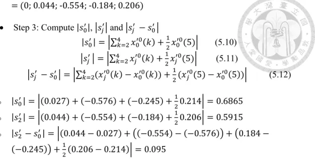
| | ∑ 4 (3.10)

∑ 4 (3.11)

∑ 4 4 (3.12)

 Compute the relative degree of incidence

| |

| | (3.13)

2. Compute the synthetic degree of incidence

ρ1j = θ ε1j + (1- θ)r1j (3.14) Whereas:

ρ1j: The synthetic degree of incidence ε1j: The absolute degree of incidence

r1j: The relative degree of incidence

With j = 2... n, (n = number of symptom. This research, n = 4) θ [0,1]

The synthetic degree of grey incidence is a numerical index that well describes the overall relationship of closeness between sequences. It reflects the similarity

(34)

26 between the zigzagged lines Xi and Xj , and also demonstrates the degree of closeness of the individual rates of change of Xi and Xj with respect to their initial points. In general, previous researchers usually take θ = 0.5. If we are more interested in the relationship between some absolute quantities, some greater value can be used as θ. In the case we are putting more emphasis on rates of change, some smaller value can be employed for θ. (Liu, S. and Lin, Y.). In the previous study scope, the researcher firstly proposed θ = 0.5 as fix value, so in this thesis scope, θ = 0.5 is chosen to compare with the same condition.

The synthetic degree of grey incidence is based on the absolute and relative degrees of grey incidence obtained earlier. The size of synthetic degree of grey incidence obtained: ρ12, ρ13… ρ1n, determine the degree in which each symptom influence the firm and conduct it to a bankrupt one. As the synthetic degree of grey incidence is higher, its corresponding variable (financial ratio) is more important.

The analysis was carried out at a single firm level then the same process with each of the consider firms will be taken into analysis. Combine the synthetic degree incidence with the sign (+/-) of each symptom, the hierarchy default probability of the sample firms are identified. About a variable j we are saying that it has a positive sign (greater is better) as it takes a higher value, the analyzed firm presents a better financial situation. Otherwise, the sign is negative (less is better). The hypothesis of variable sign will detail analyzed in the next chapter, chapter 4- Data collection). Once the default intensity of firms was determined, ROC curves (receiver operating characteristic curves) will be used to calculate the accuracy rate of prediction.

(35)

27

3.2 Over-sampling technique

3.2.1 Between-class Imbalance Problem in Date Set

Previous researches normally focused on “sample-matching” method to build the sample sets. In this method, each defaulted contractor was matched with one or two non-defaulted contractors at the year of default. However, Zmijewski (1984) pointed out that this sample-matching method led to choice-based biases and sample selection biases. If model is not built basing on entire population, the estimated coefficients will be biased. Additionally, the ultimate outcome predictions will not be guaranteed.

To avoid these biases, all available firm-quarters or firm-years for the sample period have been used in recent studies to construct the default prediction models. Hence, these models improve the accuracy of the coefficient estimates and increase the prediction power of the models compare to prior studies (Brockman and Turtle, 2003; Bharath and Shumway, 2004; Hillegeist et al., 2004; Gharghori et al. 2006;

Reisz and Perlich, 2007; Agarwal and Taffler, 2008, Tserng et al., 2011, Tsai et al., 2011, Tserng et al., 2012). Therefore, this thesis was also used all available firm- years data to develop the default prediction model.

After putting in all firm-years data, a new problem generated, that is, there was a huge discrepancy in sample size between defaulted and non-defaulted firms. It means that the number of non-defaulted samples greatly surpassed that of defaulted samples, which is referred to as between-class imbalance issue (He and Garcia, 2009). It might lead the model discriminate inaccurately healthy and non-healthy group (Chang, 2007).

In order to solve the imbalance problem, I used two over-sampling techniques in this study: replication (Japkowicz, 2000; Chawla et al., 2008) and

(36)

28 Synthetic Minority Over-sampling Technique (SMOTE) developed by Chawla et al.

(2002)

3.2.2 Replication

To tackle imbalance problem, He and Garcia (2009) put forward the idea that important information should be priority. The simple method is replication. In this research, great emphasis is put on the default samples. In other words, the default samples will be replicated several times.

In the experiment of my study, default samples in original training set were multiplied until they equal to non-default samples. It takes about 35 times replication in this research. However, to examine the models and see how good it is, I would like to replicate 1-70 times of default samples.

3.6.3 Synthetic Minority Over-sampling Technique (SMOTE)

Another way to increase number of default samples is Synthetic Minority Over- sampling Technique (SMOTE) method that was suggested by Chawla et al. (2002). The scholars proposed an over-sampling approach in which the minority class is over- sampled by creating “synthetic” examples rather than by over-sampling with replication.

This approach is inspired by a technique that proved successful in handwritten character recognition.

Firstly, the minority class is over-sampled by taking each minority class sample and introducing synthetic examples along the line segments joining any/all of the k minority class nearest neighbors. Secondly, depending upon the amount of over-sampling required, neighbors from the k nearest neighbors are randomly chosen. For example, if we use nine nearest neighbors and the amount of over-sampling needed is 200%. There are only two neighbors from the nine nearest neighbors are

(37)

29 chosen and one sample is generated in the direction of each. In this study, k is 25 for all group.

The synthetic samples are generated in following way: take the difference between the original minority sample and its nearest neighbor. Then, multiply this difference by a random number between 0 and 1, and add it to the original sample. This causes the selection of a random point along the line segment between two specific features. In this study, the minority class in the training set was over sampled at 100%, 200% until 5400% of its original size. The algorithm will be described in Figure 3.3 as follows:

Algorithm SMOTE (T; N; k)

Input: Number of minority class samples T ; Amount of SMOTE N%; Number of nearest neighbors k

Output: (N/100) * T synthetic minority class samples

1. ( If N is less than 100%, randomize the minority class samples as only a random percent of them will be SMOTEd. )

2. if N < 100

3. then Randomize the T minority class samples 4.T = (N/100) T

5.N = 100 6. End if

7. N = (int)(N/100) ( The amount of SMOTE is assumed to be in integral multiples of100. )

8. k = Number of nearest neighbors 9. numattrs = Number of attributes

10. Sample[ ][ ]: array for original minority class samples

(38)

30 11. newindex: keeps a count of number of synthetic samples generated, initialized to 0 12. Synthetic[ ][ ]: array for synthetic samples( Compute k nearest neighbors for each minority class sample only. )

13. for i ← 1 to T

14. Compute k nearest neighbors for i, and save the indices in the nnarray 15. Populate(N, i, nnarray)

16. End for Populate(N, i, nnarray) ( Function to generate the synthetic samples. ) 17. While N = 0

18. Choose a random number between 1 and k, call it nn. This step chooses one of the k nearest neighbors of i.

19. for attr ← 1 to numattrs

20. Compute: dif = Sample[nnarray[nn]][attr] − Sample[i][attr]

21. Compute: gap = random number between 0 and 1 22. Synthetic[newindex][attr] = Sample[i][attr] + gap dif 23. endfor

24. newindex++

25.N = N − 1 26. endwhile

27. return ( End of Populate. )

Figure 3.3 Synthetic Minority Over-sampling Technique

Chawla et al. (2002) argued that the outcome of SMOTE was better than the outcome of replication. In this research, I would like apply those methods in construction prediction model and compare the performance of each method.

(39)

31

3.3 ROC Curve

3.3.1 Concept and methodology of ROC curve

Assessment of predictive accuracy is an important aspect of evaluating and comparing models, algorithms or technologies that produce the predictions. Receiver operating characteristic (ROC) curves are common, widely applicable method which useful for assessing the accuracy of tests because they provide a comprehensive and visually attractive way to summarize the accuracy of predictions. So, in this research’s scope, the author proposes applying ROC curves to assess and compare the accuracy rate of default probability predictions which were applied by grey system analysis.

ROC curves, generalize contingency table analysis by providing information on the performance of a model at any cut-off that might be chosen (Green and Swets, 1966;

Hanley,1989; Pepe, 2002; Swets, 1988; Swets, 1996). In the simplest case, the model produces only two ratings (Bad/Good) which are shown along with the actual outcomes (default/no default) in tabular form. The cells in the table indicate the number of true positives (TP), true negatives (TN), false positives (FP) and false negatives (FN), respectively. FN represents a Type I error and FP represents Type II error. These fractions are presented in table 3.

 TP: a predicted default that actually occurs,

 TN: a predicted non-default that actually occurs

 FP: a predicted default that does not occur and,

 FN: is a predicted non-default where the company actually defaults.

(40)

T

P N

T

ident the f ROC decis distri sensi corne

Test

Positive Negative

Total

Figu The figu tified on a R false positiv C curve rep

sion thresh ibutions) h itivity, 100%

er, the highe

Present True Posi False Neg

ure 3.1: An ure3.1 show ROC curve ve rate (100 presents a hold. A te has a ROC

% specificit er the overa

Table 3-1

D

itive(TP) gative(NP)

n example ws how all . The true p 0-Specificity sensitivity est with pe C curve tha

ty). Therefo all accuracy

1: Types of

Default Prob

n A

a F

b T

N a + b

of ROC cu l four quan positive rate y) for differ y/specificity erfect disc at passes th

ore, the clo y of the test

error of R

bability Absent False Positiv True

Negative(TN

urve (Zweig ntities of a

e (Sensitivi rent cut-off y pair corr crimination hrough the ser the ROC is” (Zweig

OC

N ve(FP) C

N)

D

c +

g & Campbe contingenc ity) is plotte f points. “E responding (no overl e upper lef C curve is

& Campbel

Tota

a + c b + d

+ d

ell, 1993) cy table ca ed in functi

ach point o to a parti lap in the ft corner (

to the uppe ll, 1993).

32 al

c d

an be ion of on the icular two 100%

er left

(41)

33 Figure 3.2: Schematic of a ROC

3.3.2 Utilizing ROC curve to validate the model

One useful characteristic of the ROC curve is the area under the curve (AUC) clearly reflects how good the test is at distinguishing between firms with disease and those without disease. The AUC serves as a single measure, independent of prevalence that summarizes the discriminative ability of a prediction across the full range of cut-off points. The greater value of the AUC, the better the prediction is. A perfect discrimination test will have an AUC of 1.0, while a completely useless test (one whose curve falls on the diagonal line) has an AUC of 0.5. A test with an area greater than 0.9 has high accuracy, while 0.7–0.9 indicates moderate accuracy and 0.5–0.7 indicates low accuracy.

Corresponding to different circumstances of period of time (4 year data consequence) as well as X0 (sequence of characteristic data to describe the system’s behavior), the value of AUC will be calculated. And this value is the basis for evaluate and compare the accuracy of the Grey System Theory application with the different number of variables.

(42)

34

3.3 Summary

In this chapter, the author introduces the main methodology adopted in the research – grey system analysis and the way to apply this method to forecast a company default probability. By calculating synthetic degree incidence of considered firms and combine these values, the default probability of firms were identified. Beside, Over- sampling technique is used before applying Grey Theory, to address imbalance data problem. After different models are calculated, ROC curves are used to compare with the previous study.

(43)

35

CHAPTER 4: DATA COLLECTION

4.1 Data collection

4.1.1 Source and validity of data

Data in this research was gathered from COMPUSTAT Industrial File (Wharton Research Data Services) as well as the Center for Research in Securities Prices (CRSP) for construction companies of the U.S. My research concentrated on construction contractors with December fiscal year-ends by choosing firms with SIC codes between 1,500 and 1,799. Similar to the researches of Severson et al (1993) and Russell and Zhai (1996), the sample contractors include three construction categories:

 Major Group 15: Building construction, general contractors and operative builders. The construction of buildings subsection includes establishments involved in constructing residential, industrial, commercial, and institutional buildings

 Major Group 16: Heavy construction other than building construction contractors. The heavy and civil engineering subsection includes establishments involved in infrastructure projects.

 Major Group 17: Construction special trade contractors. The specialty trade contractors engaged in activities such as plumbing, electrical work, masonry, carpentry, and roofing that are generally needed in the construction of all building types.

4.1.2 Principles of collecting data

(44)

36 The selection of firm is confined in construction industry only. 92 companies were selected as participant of the research, among which 24 were defaulted. The observed period was 1972-2008. According to Chin (2009), Tserng et al. (2008), Tserng et al. (2009), there are two main criteria in data collection principle to select samples:

1. Companies which do not have financial statement for at least 5 years will be taken out of the sample.

2. Default firms are defined by CRSP delisting code of 400 and 550 to 585, which correspond to the delisting reason concerned with company failures such as bankruptcy, liquidation of poor performance.

The chosen firms must have at least five years’ data in Compustat Industrial File to ensure that all the unhealthy firms will be excluded in the population of study as well as to consider the impact of market factors to these companies in a long term.

4.1.3 Summary of the input data

This thesis have a total of 24 failed companies among 92 construction companies which were identified during the year of determination. These firm were chosen because they are suitable to two criteria above. The number of firm may be 50 but 92 firm is big enough to improve the exact of study. Besides, to find out exact number of firm, it is beyond the thesis’ limit.

Table 4.1 disclosed the name of failed firms.

(45)

37 Table 4-1: Information of the defaulted companies

ORD CODE COMPANY'S NAME DEFAULTED

YEAR

OBSERVED FIRM‐YEARS 1 60409 AMERICAN MEDICAL BLDGS INC 1989 1978 ‐1989 2 85607 ATKINSON (G F) CO/CA 1997 1985 ‐ 1997 3 63095 BANK BUILDING &EQUIP CORP AM 1989 1972 ‐ 1989

4 11901 ENTRX CORP 2004 1988 ‐ 2004

5 86933 COMSTOCK GROUP INC 1988 1984 ‐ 1988 6 22382 CERBCO INC ‐CL A 2000 1981 ‐ 2000 7 55079 MORRISON KNUDSEN CORP OLD 1995 1972 ‐ 1995 8 58641 CANISCO RESOURCES INC 1998 1982 ‐ 1998 9 10036 NEUROTECH DEVELOPMENT CORP 1990 1986 ‐ 1990 10 29621 DEVCON INTERNATIONAL CORP 2007 1987 ‐ 2007 11 11109 CEC INDUSTRIES CORP 1994 1987 ‐ 1994 12 80220 ABLE TELCOM HOLDING CORP 1999 1994 ‐ 1999 13 76432 RYAN MURPHY INC 1994 1990 ‐ 1994 14 76796 BUILDING MATERIALS HLDG CP 2007 1991 ‐ 2007 15 77334 SHOLODGE INC 2004 1992 ‐ 2004 16 77831 XXSYS TECHNOLOGIES INC 1998 1992 ‐ 1998 17 79017 TRANSCOR WASTE SERVICES INC 1997 1993 ‐ 1997 18 10227 KIMMINS CORP 1998 1986 ‐ 1998

19 79815 COFLEXIP SA 2000 1993 ‐ 2000

20 79958 DAW TECHNOLOGIES INC 2000 1993 ‐ 2000

21 82829 NESCO INC 2000 1996 ‐ 2000

22 82731 CHINA CONVERGENT CORP LTD 2000 1996 ‐ 2000 23 85606 ENCOMPASS SERVICES CORP 2001 1997 ‐ 2001

(46)

38 24 88642 DISTRIBUTED ENERGY SYS CORP 2007 2003 ‐ 2007

4.2 Data classification

4.1.4 4.2.1 Collection of Financial ratios data

Theodossiou (1991) claimed that the selection of the independent variables for a bankruptcy prediction model is the most toughing aspect of every bankruptcy because financial theory does not indicate which variables should be included in the. The forward stepwise statistical procedure has been recognized as the most popular method used in previous studies for the development of bankruptcy prediction models. Due to some specific properties of construction finance, this research’s financial ratios are collected following prior researches (Mason and Harris(1979) ; Abidali (1990); Russel and Jaselskis (1992); Cheng, J. et al (2009); Delcea, C. &Scarlat, E) which concerned to the prediction of the probability of construction firms. Besides, the selected financial ratios must involve all the aspects of a contractor finance situation and has to include the liquidity, profitability, leverage, activity of a firm and even refer to the market factor.

The last principle to select financial ratios is all of these ratios must have a predicted relationship with the default risk.

4.2.2 Clacification of selected financial ratios

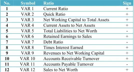
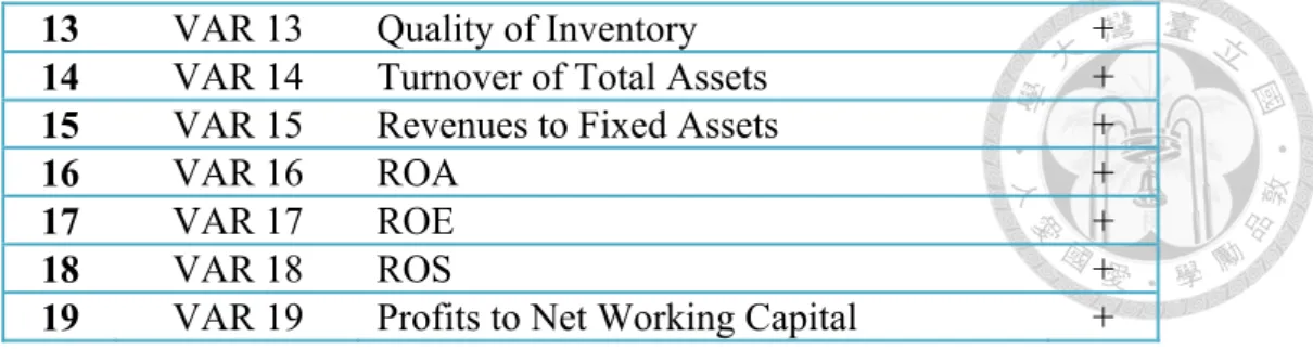
19 single financial ratios developed from financial data from 92 construction firms across a 37-year period (1972-2008) were taken into account. These ratios are classified into 4 categories of ratios (liquidity, leverage, profitability, activity) which are typically used in analyzing financial position:

(47)

39 Table 4-2: Selected ratios’ classification

1. Liquidity Ratios

No. Symbol Ratio

1 VAR1 Current Ratio

2 VAR2 Quick Ratio

3 VAR3 Net Working Capital to Total Assets 4 VAR4 Current Assets to Net Assets

2. Leverage Ratios

No. Symbol Ratio 5 VAR5 Total Liabilities to Net Worth 6 VAR6 Retained Earnings to Sales

7 VAR7 Debt Ratio

8 VAR8 Times Interest Earned

3. Activity Ratios

No. Symbol Ratio

9 VAR9 Revenues to Net Working Capital 10 VAR10 Accounts Receivable Turnover 11 VAR11 Accounts Payable Turnover

12 VAR12 Sales to Net Worth

13 VAR13 Quality of Inventory

14 VAR14 Turnover of Total Assets 15 VAR15 Revenues to Fixed Assets

4. Profitability Ratios

(48)

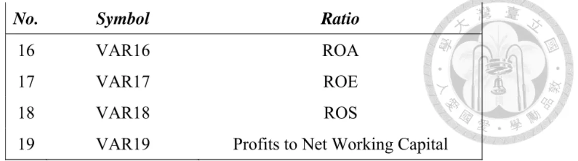
40 No. Symbol Ratio

16 VAR16 ROA

17 VAR17 ROE

18 VAR18 ROS

19 VAR19 Profits to Net Working Capital

4.3 Financial ratios’ definition

The definition and the sign of 19 major represented variables in table 4-3 below:

Table 4-3: Definition and usage ratios

Var. Ratio Definition Usage Sign

1 Current Ratio Current assets/

Current liabilities

A liquidity ratio that measures a company's ability to pay short-term obligations.

+

2 Quick Ratio (Current Assets - Inventory)/

Current liabilities

An indicator of a company's short-term liquidity measures a company's ability to meet its short-term obligations with its most liquid assets

+

3 Net Working Capital to Total Assets

(Current assets - Current

liabilities)/Total assets

Measures both a company's efficiency and its short - term financial health

+

4 Current Assets to Net Assets

Current assets/(Total assets -Current liabilities)

Indicates how effectively a company is using its assets to generate cash before contractual obligations must be paid

+

5 Total

Liabilities to Net Worth

Total liabilities /

Net worth Indicates the extent to which a company is utilizing its re-investment - 6 Retained

Earnings to Sales

Retained earnings/ Net Sales

Indicates how effectively reinvested into the company.

+

7 Debt Ratio Total liabilities / Total assets

Indicates what proportion of debt a company has relative to its assets.

-

8 Times Interest Earned

Earnings before interest and taxes / Interest charges

Measures a company’s ability to honor

its debt payments. +

灰色理論結合強化樣本技術應用於營建公司破產幾率預測之研究

National Taiwan University

Master Thesis

中華民國103年6月

June, 2014

ACKNOWLEDGEMENT

TABLE OF CONTENTS

ii

v

vii

iii

1

:

2

3.2 Over-Sampling technique………27

LIST OF FIGURES

LIST OF TABLES

CHAPTER 1: INTRODUCTION

1.1

1.3 Research objectives

1.4

1.5 T

Thesis str

ructure

CHAPTER 2: LITERATURE

2.1 Default prediction researches

2.2 Default prediction researches in construction industry

2.3 Grey system model in prediction bankruptcy probability

2.4 Summary

CHAPTER 3: METHODOLOGY

3.1 Grey system theory

3.1.1. Methods of Grey Numbers’ Generation Based on Average

3.1.2. Method of Grey Incidence Analysis

...

...

...

...

X X X X

X X X X

X X X X X

X X X X

 

 

 

  

 

 

...

...

...

...

   

   

    

   

 

 

 

  

 

 

3.2 Over-sampling technique

3.2.1 Between-class Imbalance Problem in Date Set

3.2.2 Replication

3.6.3 Synthetic Minority Over-sampling Technique (SMOTE)

3.3 ROC Curve

3.3 Summary

CHAPTER 4: DATA COLLECTION

4.1 Data collection

4.1.1 Source and validity of data

4.1.2 Principles of collecting data

4.1.3 Summary of the input data

4.2 Data classification

4.1.4 4.2.1 Collection of Financial ratios data

4.2.2 Clacification of selected financial ratios

4.3 Financial ratios’ definition