微陣列資料探勘---基因調控網路預測及基因表現與疾病關聯性分析

(1)

行政院國家科學委員會專題研究計畫成果報告

微陣列資料探勘--基因調控網路預測及基因表現與疾病關聯性分析

研究成果報告(精簡版)

計畫類別：個別型

計畫編號： NSC 99-2221-E-011-113-

執行期間： 99 年 08 月 01 日至 100 年 10 月 31 日執行單位：國立臺灣科技大學資訊管理系

計畫主持人：呂永和

計畫參與人員：碩士班研究生-兼任助理人員：邱紫怡碩士班研究生-兼任助理人員：宋政倫博士班研究生-兼任助理人員：吳宗諭博士班研究生-兼任助理人員：管金宏

報告附件：出席國際會議研究心得報告及發表論文

公開資訊：本計畫可公開查詢

中華民國 100 年 11 月 16 日

(2)

中文摘要：雖然已經有很多基因調控網路的預測方法被提出來，但這些方法都沒有考慮基因調控反應中的反應時間延遲問題。本研究提出使用動態時間校正(Dynamic time warping)為主的基因調控網路預測新方法。經由動態時間校正演算法，我們可以決定兩個基因之間的調控反應是否是延遲正相關、正相關、負相關或是不相關。我們使用基因演算法分析微陣列資料中的基因反應量的關係，建立多個候選基因調控網路；再根據’重要的基因調控關係，會出現在大多數的候選基因調控網路中’的假設，由候選基因調控網路，選出最常出現的兩基因調控關係，最後將之組合成整個基因調控網路。經由三個微陣列實驗資料組的實驗，證明我們的方法具有較高的預測敏感度及預測特異度。

中文關鍵詞：基因調控網路、基因演算法、粒子群最佳化、動態時間校正、微陣列資料分析

英文摘要： Recently, many methods have been proposed for constructing gene regulatory networks (GRNs).

However, most of the existing methods ignored the time delay regulatory relation in the GRN

predictions. In this paper, we propose a hybrid method, termed GA/PSO with DTW, to construct GRNs from microarray datasets. The proposed method uses test of correlation coefficient and the dynamic time warping (DTW) algorithm to determine the existence of a time delay relation between two genes. In addition, it uses the particle swarm optimization (PSO) to find thresholds for discretizing the microarray dataset.

Based on the discretized microarray dataset and the predicted types of regulatory relations among genes, the proposed method uses a genetic algorithm to generate a set of candidate GRNs from which the predicted GRN is constructed. Three real-life sub- networks of yeast are used to verify the performance of the proposed method. The experimental results show that the GA/PSO with DTW is better than the other existing methods in terms of predicting sensitivity and specificity.

英文關鍵詞： Gene regulatory networks； Genetic algorithms；

Particle swarm optimization； Dynamic time warping；

Microarray data analysis

(3)

微陣列資料探勘—基因調控網路預測及基因表現與疾病關聯性分析 計畫編號：NSC 99-2221-E-011-113

主持人：呂永和 {[email protected]} 國立台灣科技大學資訊管理系計畫參與人員：呂永和、吳宗諭、管金宏、邱紫怡、宋政倫

1. 中文摘要

關鍵詞：基因調控網路、基因演算法、粒子群最佳化、動態時間校正、微陣列資料分析

雖然已經有很多基因調控網路的預測方法被提出來，但這些方法都沒有考慮基因調控反應中的反應時間延遲問題。本研究提出使用動態時間校正(Dynamic time warping)為主的基因調控網路預測新方法。經由動態時間校正演算法，我們可以決定兩個基因之間的調控反應是否是延遲正相關、正相關、負相關或是不相關。我們使用基因演算法分析微陣列資料中的基因反應量的關係，建立多個候選基因調控網路；再根據"重要的基因調控關係，會出現在大多數的候選基因調控網路中"的假設，由候選基因調控網路，選出最常出現的兩基因調控關係，最後將之組合成整個基因調控網路。經由三個微陣列實驗資料組的實驗，證明我們的方法具有較高的預測敏感度及預測特異度。

2. 英文摘要

Keywords: Gene regulatory networks;

Genetic algorithms; Particle swarm optimization; Dynamic time warping;

Microarray data analysis

Recently, many methods have been proposed for constructing gene regulatory networks (GRNs). However, most of the existing methods ignored the time delay regulatory relation in the GRN predictions.

In this paper, we propose a hybrid method, termed GA/PSO with DTW, to construct GRNs from microarray datasets. The proposed method uses test of correlation coefficient and the dynamic time warping (DTW) algorithm to determine the existence of a time delay relation between two genes.

In addition, it uses the particle swarm optimization (PSO) to find thresholds for discretizing the microarray dataset. Based on the discretized microarray dataset and the predicted types of regulatory relations among genes, the proposed method uses a genetic algorithm to generate a set of candidate GRNs from which the predicted GRN is constructed. Three real-life sub-networks of yeast are used to verify the performance of the proposed method. The experimental results show that the GA/PSO with DTW is better than the other existing methods in terms of predicting sensitivity and specificity.

3. 前言

多年來，人類總是好奇究竟是哪些基因的反應或調控(gene regulatory)影響了生物的表現。微陣列技術的發明，讓生物學家減少了研究所需花費的時間，也增加研究人員了解生物基因反應的情形。以微陣列時間序列資料為例，生物學家常用它來分析基因之間彼此的互相反應(interaction)關

(4)

係，而這互相反應的關係則被稱為基因調控網路(gene regulatory networks, GRNs)。

基因之間的相互作用一般可分為，活化 (activation)( 或稱為正相關 ) 、抑制 (inhibition)(或稱為負相關)及無相關三種情形。若將一個基因視為一個節點 (node)，而兩基因之間若存在調控關係，

則可利用不循環有向圖 (directed acyclic graph)確認基因之間的調控方向。舉例來說，若 A 基因可調控 B 基因(可寫為 A→B)，而 B 基因可調控 C 基因(可寫為 B→C)，則此三基因之間可畫成一個簡單的調控圖，如圖 1。而圖 2 則為五個基因間較為複雜的調控網路圖。由圖可見，當基因數量很多時，其基因調控網路也將隨之複雜化，也大幅提高了預測其基因調控網路的難度。

圖 1. A, B, C 三基因之間的調控圖

圖 2. 五個基因之間的調控網路圖在過去的研究中，許多方法是以貝氏網路 (Bayesian networks)為基礎，預測基因的調控網路[5-7]。這些研究是將貝氏網路中的每一個節點視為一個基因，若任兩個基因被邊(edge)所連結，則代表兩基因之間有

調控關係，最後再利用因果相關(causal relationships)分析兩基因之間調控方向。

Friedman et al.[5] 就是以貝氏網路為基礎，配合統計方法中的拔靴法(bootstrap method) ，計算貝氏網路中的事後機率 (posterior probability)，以提高整體預測基因調控網路的準確度。Liu et al.[6]則是利用 semi-fixed Bayesian network 建立基因調控網路，之前許多預測基因調控網路的方法，都是藉由基因與基因之間的聯繫資訊，進而建立基因調控網路；但 Liu et al.

認為，只用基因與基因之間的聯繫資訊過於簡單，基因之間的調控應該存在其他的因素，因此利用貝氏網路配合隱藏變數 (hidden variables) 提出了 semi-fixed Bayesian network，此研究建立了 29 條酵母菌的基因調控網路，其中有 11 條關係和實際文獻所指出的調控相符。而 Li et al. [7]

則是利用基因演算法 (genetic algorithm, GA)，建立候選的貝氏網路，再以所提出的得點函數(score function)，作為基因演算法中挑選候選貝氏網路的依據，此研究正確預測了 43 條中的 31 條基因調控關係。

另外，也有許多研究以關聯規則 (association rules, AR)為基礎，進行建立基因調控網路之研究。 Creighton and Hanash[8]利用關聯規則有效的建立許多基因之間的調控關係，此方法是以關聯規則的左側(left hand side, LHS)作為調控基因，而右側(right hand side, RHS)作為被調控基因，例如：若 A 基因可調控 B 基因，

(5)

則以關聯規則表示為A→B；若 A 基因同時可以調控 B 基因與 C 基因，則可利用關聯規則表示為A→｛B, C｝。Mcinotosh and Chawla[9]提出了一個 high-confidence rule mining 的方法，此方法可有效地減少傳統列列舉(row enumeration)演算法用在微陣列資料中的計算複雜度，因此可以方便計算出基因之間的關聯規則。上述的方法大多用於預測少數基因之間的調控網路，因此 Huang et al.[10]提出 modified Bayesian network 與 modified association rule，針對大規模基因之間的調控網路進行預測；此研究發現，不管是修正過或未修正的貝氏網路，其表現皆比關聯規則還要好。

除了使用貝氏網路與關聯規則外，也有人使用其他資料探勘(data mining)方法來建立基因調控網路。例如， Linden and Bhaya[11]利用模糊規則(fuzzy rules)對基因進行模糊化，再以基因規劃 (genetic programming) 搜尋基因的調控關係。

本計劃提出一個新的混合型的方法 (hybrid method) ，利用動態時間校正 (dynamic time warping, DTW)[13] 演算法，判斷基因之時間的有無延遲反應的關係，再配合基因演算法、粒子群最佳化演算法(particle swarm optimization, PSO)[14]

及統計條件機率，建立基因調控網路，我們稱此方法為結合動態時間校正的基因/

粒子群最佳化演算法 (genetic algorithm/particle swarm optimization with dynamic time warping, 簡稱 GA/PSO with DTW)。

4. 研究方法

4.1 微陣列資料及其離散化

微陣列實驗資料可用圖 3 的矩陣表示，

11 12 1

21 22 2

1 2

m m

n n nm

m genes

M M M

n samples

M M M







圖 3. 以矩陣表示微陣列資料 其中 Mij 代表基因表現量與參考樣本的表 現量的關係，Mij>0 代表基因表現過量，

Mij<0 則表示基因表現量不足。為方便分析，我們以公式(1)將微陣列資料離散化，

而公式(1)中的門檻值 θ 則是以粒子群最佳 化演算法求得。所以 Xij=1 表示基因表現過量，餘此類推。

1, ,

0,

ij

ij ij

M

X M



 

   

 其它

(1)

4.2 建立基本基因調控組合

由於最小的基因調控網路就是兩個基因之間的調控關係；因此，我們藉由兩個基因之間的調控關係往外擴張，建立整個基因調控網路。藉由基因調控組合列表，我們可以列出所有兩個基因之間的基因調控組合。表(1)為 5 個基因的 10 種基因調控組合。

表 1. 基因調控組合表

Combination ID 1 2 3 4 5

Gene1 Gene1 Gene1 Gene1 Gene2 Gene2 Gene3 Gene4 Gene5 Gene3

Combination ID 6 7 8 9 10

Gene2 Gene2 Gene3 Gene3 Gene4 Gene4 Gene5 Gene4 Gene5 Gene5

4.3 判定基本基因組的調控型態

(6)

我們以動態時間校正及相關係數分析，判斷基本基因組之間的調控型態。其方法如圖(4)的流程圖所示。

圖 4. 基因組(G1, G2)的控制型態判斷流程圖

圖(4)中首先計算兩個基因的多時間點的表現量之間的相關係數；若其大於 0，

則判斷為正向調控；若小於 0 則以 DTW 演算法將兩個基因的多時間點表現量時間序列（向量）作轉換，找出相關係數最大的轉換後向量，再以相關係數判斷其為時間延遲正向調控、負調控或無調控。

4.3 以基因演算法產生多個候選調控網路 使用整數編碼代表候選基因調控網路，如圖(5)所示，位置代表基因組的編號，'1'代表選取，'0'代表不選取。參考表 (1)的編碼，可由左邊的染色體建立右邊的基因調控圖。

圖 5. 染色體編碼

基因演算法的以單點交配(single point crossover)及平均突變(uniform mutation)改變染色體。適應函數值(fitness value)是以代表基因控制可信度的一個稱為 R-value 的參數表示，R-value 的公式如公式(2)所示。

 1 2

1 2 1 2

1 2

1 1

1 2 1 2

1 1

,

( 1 1) ( 1 1)

, ( , ) belongs to or ,

( 1) ( 1)

( 1 1) ( 1 1)

, otherwise;

( 1) ( 1)

i i

i i i i

i i

i i i i

i i

R G G

P G G P G G

G G A TD

P G P G

P G G P G G

P G P G



       

 

   

        

 

   



(2)

 2 1

1 2 1 2

2 1

2 2

1 2 1 2

2 2

,

( 1 1) ( 1 1)

, ( , ) belongs to or ,

( 1) ( 1)

( 1 1) ( 1 1)

, otherwise.

( 1) ( 1)

i i

i i i i

i i

i i i i

i i

R G G

P G G P G G

G G A TD

P G P G

P G G P G G

P G P G



       

 

   

        

 

   



其中(G1,G2)順序組是將基因 G2 的表現向量向右位移一個時間單位，代表基因 G1 影響 G2，反之亦然。如圖(6)示意圖所示。

圖 6. 基因反應順序組

公式(2)中的 A 代表正向調控、TD 代表時間延遲調控、"其它"代表負調控。而一個候選調控網路的適應函數值是每組基本基因調控組的兩個 R-value 取大者，再對所有調控組取 R-value 的平均值。

4.4 合成調控網路

以基因演算法產生多個候選調控網路後，選取出現次數較多的基因組，建立最後的基因調控網路，此部分使用卡方同質性檢定，決定所選取基因組的個數。而最後基因的調控方向，則以基因組在不同的候選調控網路中的 R-value，以排列檢定 (Permutation Test)的方法決定。

5. 本方法的績效

我們以常用的敏感度(Sensitivity)及特異

(7)

度(Specificity) 為比較標準，以酵母菌調控子網路（yeast transcriptional cell cycle sub-network）為測試資料建立如圖(7)的調控網路，圖(7)的左邊(a)為實際文獻中所報告的調控網路，右邊(b)為本方法所預測的調控網路。實線代表正確預測、虛線代表錯誤預測。

圖 7. 所預測的調控網路

與現有方法比較如表(2)所示，

表 2. 效能比較表

Algorithms P C Sensitivity Specificity K2 12 1 1/18=0.0556 1/12=0.0833 SEM 16 4 4/18=0.2222 4/16=0.2500 k-DBN 27 5 5/18=0.2778 5/27=0.1852 SSEM 29 11 11/18=0.6111 11/29=0.3793 GA/PSO with

DTW

30 14

14/18=0.7778 14/30=0.4667

其中 sensitivity 代表所預測正確的調控個數與所發表的調控個數的比值，specificity 代表預測正確的調控個數與所有預測的所有調控個數的比值。由表(2)所示，我們的方法在兩個比較標準上，都比其它的方法好。

6. References

[1] M. Schena, D. Shalon, R.W. Davis, P.O. Brown, Quantitative Monitoring of Gene Expression Patterns with a Complementary DNA Microarray,

Science, 270 (1995) 467-470.

[2] C.-P. Lee, Y. Leu, A novel hybrid feature selection method for microarray data analysis, Appl. Soft.

Comput., 11 (2009) 208-213.

[3] X. Zhou, D.P. Tuck, MSVM-RFE: extensions of SVM-RFE for multiclass gene selection on DNA microarray data, Bioinformatics, 23 (2007) 1106-1114.

[4] Z.S.H. Chan, L. Collins, N. Kasabov, Bayesian learning of sparse gene regulatory networks, Biosystems, 87 (2007) 299-306.

[5] S.P. Li, J.J. Tseng, S.C. Wang, Reconstructing gene regulatory networks from time-series microarray data, Physica A, 350 (2005) 63-69.

[6] C. Creighton, S. Hanash, Mining gene expression databases for association rules, Bioinformatics, 19 (2003) 79-86.

[7] Z. Huang, J. Li, H. Su, G.S. Watts, H. Chen, Large-scale regulatory network analysis from microarray data: modified Bayesian network learning and association rule mining, Decis.

Support Syst., 43 (2007) 1207-1225.

[8] T. McIntosh, S. Chawla, High Confidence Rule Mining for Microarray Analysis, IEEE/ACM Trans.

Comput. Biol. Bioinform., 4 (2007) 611-623.

[9] H.-C. Wang, Y.-S. Lee, Gene Network Prediction from Microarray Data by Association Rule and Dynamic Bayesian Network, Lecture Notes in Computer Science, 3482 (2005) 309-317.

[10] N. Friedman, M. Linial, I. Nachman, D. Pe'er, Using Bayesian Networks to Analyze Expression Data, J. Comput. Biol., 7 (2000) 601-620.

[11] S. Kim, S. Imoto, S. Miyano, Dynamic Bayesian network and nonparametric regression for nonlinear modeling of gene networks from time series gene expression data, Biosystems, 75 (2004) 57-65.

[12] S.Y. Kim, S. Imoto, S. Miyano, Inferring gene networks from time series microarray data using

(8)

dynamic Bayesian networks, Brief. Bioinform., 4 (2003) 228-235.

[13] T.-F. Liu, W.-K. Sung, A. Mittal, Model gene network by semi-fixed Bayesian network, Expert Syst. Appl., 30 (2006) 42-49.

[14] M. Zou, S.D. Conzen, A new dynamic Bayesian network (DBN) approach for identifying gene regulatory networks from time course microarray data, Bioinformatics, 21 (2005) 71-79.

[15] Z.S.H. Chan, I. Havukkala, V. Jain, Y. Hu, N.

Kasabov, Soft computing methods to predict gene regulatory networks: An integrative approach on time-series gene expression data, Appl. Soft.

Comput., 8 (2008) 1189-1199.

[16] R. Eriksson, B. Olsson, Adapting genetic regulatory models by genetic programming, Biosystems, 76 (2004) 217-227.

[17] T. Tian, Stochastic models for inferring genetic regulation from microarray gene expression data, Biosystems, In Press, Corrected Proof (2009).

[18] R. Linden, A. Bhaya, Evolving fuzzy rules to model gene expression, Biosystems, 88 (2007) 76-91.

[19] M.S. Dasika, A. Gupta, C.D. Maranas, J.D. Varner, A Mixed Integer Linear Programming (MILP) Framework for Inferring Time Delay in Gene Regulatory Networks, Pac. Symp. Biocomput., 9 (2004) 474-485.

[20] R. Bellman, R. Kalaba, On adaptive control processes, Automatic Control, IRE Transactions on, 4 (1959) 1-9.

[21] C. Myers, L. Rabiner, A. Rosenberg, Performance tradeoffs in dynamic time warping algorithms for isolated word recognition, IEEE Trans. Acoustics, Speech, and. Signal Proc., 28 (1980) 623-635.

[22] R. Jayadevan, R.K. Satish, M.P. Pradeep, Dynamic Time Warping Based Static Hand Printed Signature Verification, Journal of Pattern Recognition Research, 4 (2009) 52-65.

[23] D.J. Burr, Designing a Handwriting Reader, IEEE

Trans. Pattern Analysis and Machine Intelligence, 5 (1983) 554-559.

[24] J. Kennedy, R. Eberhart, Particle swarm optimization, Proceedings of the 1995 IEEE International Conference on Neural Networks, 4 (1995) 1942-1948.

[25] M. Clerc, J. Kennedy, The particle swarm - explosion, stability, and convergence in a multidimensional complex space, IEEE Trans. Evol.

Comput., 6 (2002) 58-73.

[26] Y. Shi, R. Eberhart, A modified particle swarm optimizer, Proceedings of the 1998 IEEE International Conference on Evolutionary Computation, (1998) 69-73.

[27] P.T. Spellman, G. Sherlock, M.Q. Zhang, V.R. Iyer, K. Anders, M.B. Eisen, P.O. Brown, D. Botstein, B.

Futcher, Comprehensive Identification of Cell Cycle-regulated Genes of the Yeast Saccharomyces cerevisiae by Microarray Hybridization, Mol. Biol.

Cell, 9 (1998) 3273-3297.

[28] B. Futcher, Transcriptional regulatory networks and the yeast cell cycle, Curr. Opin. Cell Biol., 14 (2002) 676-683.

[29] E.N. Manderson, M. Malleshaiah, S.W. Michnick, A novel genetic screen implicates Elm1 in the inactivation of the yeast transcription factor SBF, PLoS One, 3 (2008) e1500.

[30] M.D. Petroski, R.J. Deshaies, Context of multiubiquitin chain attachment influences the rate of Sic1 degradation, Mol Cell., 11 (2003) 1435-1444.

7 計畫成果自評

(1) 研究內容與原計畫相符程度

由於原提計畫為兩年，但只通過一年，本研究內容與原提案計畫的第一年內容相符。

(2) 預計達成目標狀況

(9)

本計畫所提之研究目標，都能有效地達成。

(3) 研究成果的學術或應用價值

本研究成果具有學術及應用價值。

(4) 是否適合在期刊上發表

本研究的結果；；"Constructing gene regulatory networks from microarray data using GA/PSO with DTW"，已被 Applied Soft Computing, SCI: Impact Factor 2.10 所接受，另一結果："A Gene Selection Method for Microarray Data Based on Sampling"發表在

Computational Collective Intelligence 的國際會議上（Second international conference, ICCCI 2010, Kaohsiung, Taiwan, November 2010)，會議論文由 Springer 的 LNAI 6422 所收錄，具有不 錯的能見度。

(5) 本研究成果具有實用性，可以推廣使用。

(10)

An Effective Stock Portfolio trading Strategy using Genetic Algorithms

and Weighted Fuzzy Time Series

Yungho Leu*, Tzu-I Chiu

National Taiwan University of Science and Technology

[email protected], M9809116 @mail.ntust.edu.tw

Abstract

Investments in a stock market may incur risk. To reduce the risk of an investment, many portfolio selection methods have been proposed. By buying several stocks together, a portfolio selection method aims at maximizing the return of an investment given a predefined risk level. To build an optimal stock portfolio, one needs to select stocks and decide the proportion of the capital on each stock. Also, it is very important to decide when to buy or sell a stock portfolio.

.

In this paper, we present a genetic algorithm to build stock portfolios. The proposed method comprises a genetic algorithm and a weighted fuzzy time series. The genetic algorithm is used to construct an optimal portfolio while the weighted fuzzy time series is used to predict the return of the portfolio which in turn is used to formulate the fitness function of the genetic algorithm.

Furthermore, we propose the periodically checking and stop-loss point policies to decide selling and buying time points of the stock portfolio. The experiments on the stocks of Taiwan 50 show that the proposed method outperforms the Taiwan 50 index and the TAIEX index in terms of the 7-year average return rate.

Keywords: Genetic Algorithms, Weighted Fuzzy Time Series, Stock Portfolios, Selling and Buying Time Points

1. Introduction

One important problem in investment is to distribute the capital of the investment among different assets so as to reduce the investment risk. In 1952, Markowitz proposed a portfolio model [1] which uses the means and variances of the returns of assets to express the tradeoff between the return and risk of a portfolio. The model is expressed as an optimization problem with two conflicting goals. On one hand, the risk of a portfolio, represented by the variance on the returns of different assets, needs to be minimized, while on the other hand, the expected return of the portfolio needs to be maximized. Markowitz portfolio model has found wide applications in portfolio selection and asset allocation.

While it is powerful, it is a single trading point model

meaning that it concerns only on how to construct a portfolio but not on when to sell or buy a portfolio.

In this paper, we propose a method for not only constructing a portfolio but also trading the constructed portfolio. The proposed method comprises a genetic algorithm and a fuzzy time series model. The fuzzy time series model is used to predict the prices of the constituent stocks in a market, which in turn are used by the genetic algorithm to construct efficient portfolios.

We also set up policies to trade the portfolios. By setting a periodically checking and a stop-lose point policies, we try to find a proper trading time point for a portfolio.

A portfolio trading system to realize the proposed method is implemented in JAVA. Through experiments on the stock prices in Taiwan 50, we show that the return rate of the proposed method is significant higher than the market and the buy and hold method.

The rest of the paper is organized as follows. In Section 2, we discuss the related work. In Section 3, we give the details of the proposed algorithm. Section 4 presents the experimental result and Section 5 concludes this paper.

2. Related work

In this section, we will discuss the related work of this paper, which includes the research on stock portfolios, genetic algorithms and the fuzzy time series model.

2.1 Research on stock portfolios

Four important issues related to stock portfolios are stock selection, asset allocation, trading point and trading strategy. We will review the related works in the following.

Wen et. al. proposed to use support vector machine (SVM) and Box Theory to obtain the upper and the lower bounds of the price oscillation box of a stock with a SVM algorithm. If the current price of the stock is higher than the upper bound, a buying signal is given.

Conversely, if the price becomes lower than the lower bound of the box, a selling signal is given. Through

(11)

experiment, they showed their system is better than the buy and hold policy. However, their system focused on single stock trading.

Chen et. al. [4] formulated the traditional portfolio problem as an investment strategy portfolio problem.

They also proposed a combination genetic algorithm (CGA) to solve the investment strategy portfolio problem. Their experiments showed that the solution of CGA is better than uniform allocation.

2.2 Fuzzy Time Series

Based on fuzzy sets [5], fuzzy time series model was proposed by Song and Chissom in 1993 [6]. According to Zadeh’s definition, a fuzzy set can be defined in the following. Let U, denoted by U={u₁,u₂,…,u_n}, be the set of universe of discourse. A fuzzy set A on U can be defined as follows:

(1) where

, and

In Equation (1), f_A is the membership function of fuzzy set A, and f_A(u_i) denotes the membership value of element u_iin fuzzy set A.

According to [6], the following definitions of fuzzy time series are given.

Definition 1. Let Y(t) (t =…,0,1,2,…), a subset of R¹, be the universe of discourse in which fuzzy sets f_i(t) (i = 1,2...) are defined. If F(t) is a collection of f_i(t), F(t) is called a fuzzy time series defined on Y(t).

Definition 2. If for any f_j(t)F(t), there exists an f_i(t-1)F(t-1), such that there exists a fuzzy relation Rij(t, t-1) and f_j(t)=f_i(t-1)。R_ij(t, t-l) where ‘。’ is the max-min composition, F(t) is said to be caused by F(t-1) only, and it can be represented by F(t-1)→F(t).

Definition 3. If F(t) is caused by F(t-1), F(t-2),…,and F(t-n), F(t) is called a 1-factor n-order fuzzy time series, and it can be represented by:

F_t-n, …, F_t-2, F_t-1→F_{t .} (2) 2.3 Weighted Fuzzy Time Series

The weighted fuzzy time series model was proposed by Yu in 2005 [2]. Yu argued that recent fuzzy rules should play more important roles in prediction than the older fuzzy rules. Therefore, this model gives more weights to the recent fuzzy rules than the weights to the older rules.

2.4 Genetic algorithms

Genetic algorithms (GAs), proposed by John Holland in 1970, provide a learning method motivated by analogy to biological evolution [3]. To find the optimal

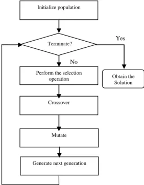
solution for a specific problem, a GA encodes the solutions to the problem into chromosomes. Each chromosome represents a feasible solution to the problem. A fitness function is devised to evaluate the goodness of the solutions to the problem. Better solutions will have higher fitness values. Through crossover and mutation operations, the GA generate a successor generation from the existing generation. With the selection operation, each successor generation contains solutions which are better than those of its predecessor generations. After evolving enough generations, GAs usually finds a good solution to the problem. Note that the solution found by GAs may not be the optimal solution. The flowchart of a prototypical genetic algorithm is shown in Fig. 1.

Figure 1. The flowchart of a prototypical genetic algorithm

3. The proposed Method

In this section, we give the details of the proposed method for trading stock portfolios.

3.1 Stock selection and investment allocation

We integrate the stock selection and investment allocation into the integer encoding method of the GA.

In the encoding method, we select at most five stocks in Taiwan 50 to construct a portfolio. For each selected stock, a weight for it in the investment is also selected.

In the following, we use examples to illustrate the encoding method, the crossover and the mutation operations.

3.1.1 Encoding

Yes s No

Initialize population

Generate next generation Perform the selection

operation

Crossover

Mutate

Obtain the Solution Terminate?

(12)

Table 1 shows a chromosome of the GA. In this encoding, we keep a table to track the mapping between the title of each stock in Taiwan 50 and an assigned integer ranging between 1 and 50. To generate a chromosome, a random number generator is called to generate five positive integers each between 1 and 50.

Along with each selected stock, the random number generator is called to generate an integer (allocation number) ranging between 1 and 100. As illustrated in Table 1, the allocation numbers are normalized to generate the weight for each stock in the portfolio.

Table 1. Encoding of the GA Stock

no. 7 30 24 15 5

Title of the stock

Chang Hwa Bank

Chung- hwa Telecom Co.

LiteOn Technol ogy Co.

China trust

China steel

Allocat

ion no. 10 25 15 30 35

proport

ion ^0.087 ^0.2174 ^0.1304 ^0.2609 ^0.3043 3.1.2. Crossover

Table 2 shows a single-point crossover operation of the GA. In table 2, a position, between 2 to 5, is chosen.

Then, the strings of the two parents, starting from the chosen position to the end of the strings, are swapped.

Table 2. The crossover operation parents

Stock no. 7 30 24 15 5

Alloc. no. 10 25 15 30 35

Stock no. 8 10 35 16 2

Alloc. no. 15 25 20 35 40 Offsprings

Stock no. 7 30 35 16 2

Alloc. no. 10 25 20 35 40

Stock no. 8 10 24 15 5

Alloc. no. 15 25 15 30 35

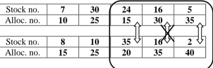
Note that in swapping the strings, no duplicate stocks are allowed. When duplicate stocks are found, they are not swapped. One example is shown in Table 3 in which stock number 16 is not swapped.

Table 3. An example of swapping conflict

Stock no. 7 30 24 16 5

Alloc. no. 10 25 15 30 35

Stock no. 8 10 35 16 2

Alloc. no. 15 25 20 35 40 3.1.3 Mutation

Single-point mutation is adopted in the GA. To perform a single-point mutation, first a position in the string is chosen. Then, the stock number and its allocation number are changed randomly. Note that the duplication in stock numbers needed to be checked to prevent duplicate stock numbers. Table 4 shows an example of mutation.

Table 4. Single-point mutation parent

Stock no. 7 30 35 16 2

Alloc. no. 10 25 20 35 40

offspring

Stock no. 7 30 5 16 2

Alloc. no. 10 25 15 35 40

3.2 Return rate prediction

The return rate of a portfolio can be calculated by knowing to price of each of its constituent stock. To predict the stock price, we use the weighted fuzzy time series model.

For each portfolio generated by the GA, the following procedure is followed to predict its expected return rate：

Step 1：Define the fuzzy set of each stock price

From the historical data of the stock prices, find the range of the universe of discourse U={ Dmax, Dmin}.

Then, partition U into n equal-length partitions, denoted by u₁,u₂,…,un, respectively. Afterwards, define n fuzzy sets as follows:

.

Step 2：Fuzzify the historical data

To fuzzify the historical data, we map the stock price of a stock at date t to its corresponding fuzzy set. The mapping rule is that if the closing price of the stock lies in the interval of u_k , then the closing price is mapped to A_k.

Step 3：Construct fuzzy logical relationships (FLRs) With the fuzzified historical data, we can construct the fuzzy logical relationships (FLRs) depending on the need of the prediction. Suppose that we want to predict the closing price of a stock based on its previous day’s closing price. If the fuzzified data of two consecutive dates t-1 and t are A_i and A_j, respectively. Then, the following FLR is constructed:

FLR：Ai →Aj

Step 4：Find the group of FLRs for the prediction Construct the left hand side of the FLR for the day of

prediction (i.e., the day to perform the prediction). With this FLR, search for matched FLRs from the FLR

(13)

historical database. Then, put them together into a set called fuzzy logical relationship group (FLRG). A matched FLR is an FLR whose left hand side matches the left hand side of the FLR of the prediction day.

Step 5：Predict the stock price

The predicted value is the weighted sum of the right hand side of the rules in FLRG. The following example illustrates this step. Assume that the FLR database is as follows:

(t=1) A₁ →A₁ , (t=2) A₁ →A₂ , (t=3) A2 →A1 , (t=4) A₁ →A₁ , (t=5) A₁ →A₁ .

Assume that the left hand side of the predicting day (t=6) is A₁. Then the defuzzified values of the matched FLRs and their weights are shown as follows:

(t=1) A1 →A1 weight 1, (t=2) A₁ →A₂ weight 2, (t=4) A₁ →A₁ weight 3, (t=5) A1 →A1 weight 4.

Finally the value of day 6 is calculated according to Equation (2) as follows:

Predicted value= A2 A1 (2)

Note that A₁ is the mid-point value of its corresponding interval u1.

3.3 Fitness function

The GA uses fitness function to select better chromosomes to survive in the evolution process. In this stock portfolio trading problem, the fitness function is the expected return rate of a portfolio. The expected return rate of a portfolio is the weighted sum of the returned rates of its constituent stocks, which is shown in Equation (3).

Fitness value = , (3) where F_i(t+5) is the predicted price of stock i at date t+5; N_i(t) is the price of stock i at date t; C_i is the proportion of the investment on stock i. Note that we assume that there are 5 stocks in each portfolio and the new portfolio is constructed at date t.

3.4 Stock portfolio trading Strategy

The trading strategy comprises two policies:

periodically checking and stop-lose point checking.

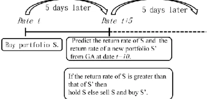
3.4.1 Periodically checking

Suppose that we buy a portfolio S at date t. Then five days later at date t+5, we generate a new portfolio S’

with the best expected return rate, and compute the

expected return rate of portfolio S. If the expected return rate of the new portfolio S’ is greater than that of S, we sell S and buy S’; otherwise, we hold S. The scenario is shown in Fig. 2.

Figure 2. Trading strategy at transaction time points 3.4.2 Stop-lose point checking

When the market plunges abruptly, the loss of a stock portfolio may be huge if it is not sold promptly. To cope with the volatility of the market, we set a stop-lose point which is the amount of return loss beyond which we sell the stock portfolio. Two stop-lose points are set for the proposed strategy. They are daily stop-lose point and accumulated stop-lose point. The former is for the loss in a day, after opening and before closing of the market, while the later is for the accumulated loss within five consecutive trading days. When a stop-lose point is reached, we sell the stock portfolio and buy another stock portfolio at the next trading day. The stop-lose point is set at -7% in the following experiment. The scenario of stop-lose point is shown in Fig. 3.

Figure 3. Trading strategy with stop-lose point

4. Experiments and Analysis

To show the viability of the proposed strategy, we implement a trading system in JAVA. The system is composed of a GA and a weighted fuzzy time series model. With the predicted return rates of portfolios by the weighted fuzzy time series, the GA select best stock portfolios for investments. In the following, we report the experimental data, benchmarking indices and the experimental results.

4.1Experimental data

(14)

The experimental data are the prices of stocks in Taiwan 50. Taiwan 50 comprises top-weighted 50 constituent stocks in TAIEX.

The selected data are the closing prices of the 50 stocks from January 2, 2004 to December 31, 2010.

The data contain 1743 stock prices. We use sliding window model to construct stock portfolios. The experiments are performed year by year. In each year, the first 3 months’ data are used only as historical data for constructing portfolios of the following 9 months.

Therefore, there is no investment for our strategy in the first 3 months. The experimental results are summarized annually.

4.2 Benchmarking indices

4.2.1 TAIEX

Taiwan Stock Exchange Capitalization Weighted Stock Index, abbreviated as TAIEX, is compiled by Taiwan Stock Exchange Co., Ltd. [8]. It is calculated by Equation (4):

Index = aggregate market value / Base value of the current day * 100, (4)

where the aggregate market value is the summation of the market values obtained by multiplying the traded price of each constituent stock by the issued shares of the current day. The initial base value of the market is the annual average market value of Taiwan stock market in 1966. The base value of the market is updated when new constituent stock is added or an existing constituent stock is deleted [8]. The performance of TAIEX gives the investors an idea about the performance the market as a whole and can be used as a benchmark for the performance of stock portfolios.

4.2.2 Taiwan 50 index

Taiwan 50 index is an index of the top-fifty capitalization stocks in TAIEX. Its constituent companies are usually stable and highly performing companies. Therefore, the return rate of Taiwan 50 index is usually higher than that of TAIEX.

4.3 Experimental environment and parameter setting

The experiment is performed on a PC with Microsoft Windows XP operating system. The algorithm is implemented in JAVA. The parameters of the GA are shown in Table 5. Note that the transaction cost in a portfolio transaction includes 1.425% fee for the seller and buyer each and 3% tax, which total to roughly 6%.

Table 5. Parameter setting

Population size 10

No. of iteration in GA 1000 Selection method Roulette wheel

Crossover Single-point crossover

Crossover rate 0.8

Mutation Single-point mutation

Mutation rate 0.1

Transaction cost 6 ‰ *

*: Transaction cost= 1.425 ‰ 2 3 ‰ 6 ‰.

4.4 The experimental results

To evaluate the performance of the proposed strategy, return rates are compared. To calculate the return rates, the following rules are followed:

1. The proposed strategy：Start trading on April 1, and calculate the accumulated return rate at the end of the year.

2. TAIEX: Subtract the index value on April 1 from the index value at the end of the year; divide the result by the index value on April 1.

3. Taiwan 50 index：Same as TAIEX except that Taiwan 50 index is substituted for TAIEX index.

4.4.1 Experimental results

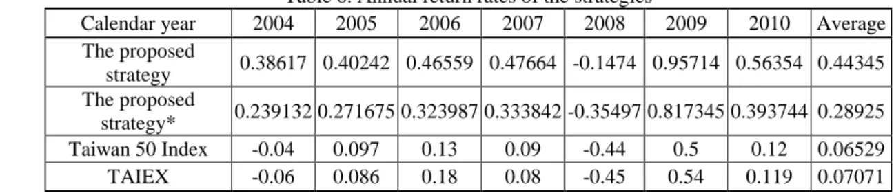
The comparisons are shown in Table 6 and are depicted in Fig. 4. From Table 6, it shows that the 7-year average return rate of the proposed strategy is 0.4434, which is much higher than those of TAIEX and Taiwan 50 index. From Fig. 4, we observe that in the year of 2008, when the global economic crisis occurred due to the subprime mortgage problem, the proposed strategy prevents big loss due to the stop-lose point checking policy. Also, the periodically checking policy attains better return rates with better portfolios in the years other than 2008. Note that in the experiment we have the following assumptions: