稠密顆粒材料在無邊界均勻剪力流之穩定分析

國立臺灣大學工學院土木工程學系 碩士論文

Department of Civil Engineering College of Engineering

National Taiwan University Master Thesis

稠密顆粒材料在無邊界均勻剪力流之穩定分析

Stability analysis of unbounded uniform dense granular shear flows

賴政佑 Jeng-You Lai

指導教授：楊德良 博士 Advisor: Der-Liang Young, Ph.D.

中華民國 98 年 7 月

July, 2009

Table of contents

誌謝 III

摘要 IV

Abstract V

Figure list VI

Table list IX

Symbols X

Chapter 1 Introduction 1

1.1 Motivation 1

1.2 Literature survey 2

1.3 Organization of thesis 7

Chapter 2 Mathematical model 11

2.1 Governing and constitutive equations 11

2.2 Basic-state derivation and non-dimensional process 14

2.2.1 Basic-state derivation 14

2.2.2 Non-dimensional process 15

2.3 Linear perturbation process 17

2.4 Fourier mode process 21

Chapter 3 Method of stability analysis 26

3.1 Criterion of asymptotic stability analysis 26 3.2 Criterion of transient stability analysis 27 3.3 Criterion of transient stability analysis for non-layering

modes

29

Chapter 4 Results and discussions 31

4.1 The spatially uniform mode for purely kinetic model 31

4.2 Layering modes for purely kinetic model 33

4.2.1 Results for asymptotic stability analysis 34 4.2.2 Results for transient stability analysis 36 4.3 Non-layering modes for purely kinetic model 42 4.3.1 Results for asymptotic stability analysis 42 4.3.2 Results for transient stability analysis 43

4.4 Results for frictional-kinetic model 47

Chapter 5 Conclusions and future works 74

5.1 Conclusions 74

5.2 Future works 76

References 77

Appendix A Elements of M(t) 79

Appendix B Theoretical proof of non-existence of the neutral stability

curve for layering modes 81

Personal information of author 85

誌 謝

終於將這一篇文章完成了，在此需要感謝的人實在是太多了。首先，我要感謝我最尊敬的 恩師－楊德良老師。在兩年的研究時光中，我看到楊老師對於研究學問上有著非常認真且嚴 格態度，這深深影響著我，使我明白做一件事情不單單只是完成而已，在好還要更好的要求 下使我自己還有更進步的空間。整個研究團隊在楊老師的耐心教導下，除了研究產量不斷地 提升精進外，整個團隊的向心力也緊密地凝聚在一起，使我這兩年來備受學長姐的溫暖關懷 與指導。

我也非常感謝我的博士後指導－陳文瑤博士。雖然一開始對於陳博士類似壓榨的指導方式 感到痛苦與不適，但是隨著時間過去，我才徹底體會他的苦心。在他的堅持下，我的潛能得 以逼迫出來，對於整體的研究工作除了具有一定份量外，品質更是受到嚴格的審核。另外，

我也特別感謝陳博士對我的包容與諒解，在這兩年的研究歲月中，有過迷惘與不知所措的時 刻，曾幾何時有懷著一走了之的逃避念頭，但是，由於陳博士細心的分析與開導，並且不斷 的激勵著我向前，使我重拾著信心繼續下去，感謝他的堅持，讓我有這樣的成就。

我也感謝口試委員－楊馥菱老師，在這碩士生涯中曾受過她的教導，楊馥菱老師曾對於我 做研究的態度給予一些建議，至今都讓我無法忘懷且受用無窮。我也非常感謝口試委員－廖 清標老師與古孟晃學長，對於論文的缺失加以糾正，使我的論文能夠像樣地拿出去。我也感 謝整個研究團隊，非常感謝沈立軒學長常貼心、耐心且不吝嗇地開導著迷網的我，也感謝古 孟晃學長、林英傑學長曾對我於研究過程的建議與幫助，還有感謝其他博班的學長姐們給予 我的幫忙與關懷。我也特別感謝同一間的兩位博士學長－陳壯弦學長與吳建廷學長，除了常 麻煩你們指導外，我真的在你們身上學到很多我所欠缺的事物。感謝曾港錫學弟對於我口試 期間的大力幫忙，還有兩位同時期進入碩班的同學－李建興同學與吳佳珊同學，感謝有你們 的陪伴與扶持，使我這兩年的研究生涯得以完整。

最後感謝爸、媽還有家人的全力支持使我無後顧之憂，也感謝女友雅瓊在我趕論文忙碌期 間，對我貼心的照顧與細心的幫忙，你們的支持是我最大的精神支柱。

摘要

本篇論文是利用線性穩定理論去分析稠密顆粒材料在均勻剪力下之無邊界的流況行為。

此分析是根據修正後的運動理論組成方程式去進行稠密狀態下之研究，這邊採用乾顆粒，每 一個顆粒都為等大小之光滑非彈性球體。在本篇主要進行的研究，乃利用漸進與暫態穩定理 論方法去分析完全運動模型在稠密狀態下的情形。暫態現象可以實用性地提供對於有限振幅 之發展是否藉由瞬間的觸發而產生的。此線性擾動系統可由凱文模式去得解，凱文模式的幾 何意義為擾動波向量會因均勻剪力流況而發生旋轉現象。在空間獨立模式下，整個系統將隨 著時間演進而呈現不穩定的現象。系統在沒有流向方向的擾動波情況下，會呈現漸進穩定的 現象，另外證明了邊界穩定曲線不可能存在此組成律所定義的範圍內。發現當固體體積比率 與恢復係數增加時，初始暫態成長率與最大的暫態成長將會隨之提高。但是在初始縱向擾動 波增加時，只有初始暫態成長率會跟著提升，而最大的暫態成長卻反之下降。當擾動波沒有 限定只能縱向傳遞時，暫態函數隨著時間的演進將會出現多重的高峰且最大的暫態成長值將 明顯地隨著初始縱向擾動波減少而跟著提高。這是由於本研究的系統矩陣乃為非正則矩陣，

此將造成初始暫態成長率在極短的瞬間有了正的值，因此可向上發展，且非正則矩陣也是造 成暫態成長函數有出現極大值與震盪發生的可能。另外，藉由初始條件下各分量隨時間之發 展，任何一個分量在不同時間下之主宰情形亦可被觀察出來。我們在最後將討論加入半線性 應力知結果。由於此結果呈現非常混亂的情形，我們依據此結果進而提出對於此修正後的組 成方程式之相關建議。

關鍵字：稠密顆粒流、完全運動模型、漸進穩定、暫態穩定、分層模式、非分層模式。

Abstract

This thesis presents a linear stability analysis of unbounded uniform dense granular shear flows.

The analysis is based on the revised constitutive equations of the kinetic theory (Savage 2008) for dry, identical spherical, smooth and inelastic particles in the dense state. In the present work, the purely kinetic model in dense state has been studied by asymptotic and transient stability analyses.

Transient phenomena can provide a viable way to trigger finite amplitude effects. The solution of the linear perturbed system is obtained by the Kelvin-mode which means that the wavenumber vector of the disturbances is turned by the mean shear flow. The result of spatially uniform mode is unstable when time proceeds. Disturbances of zero streamwise wavenumber are always stable by the asymptotic results and the marginal stability curve has proved that it does not exist. As the solids volume fraction and coefficient of restitution are increased, the initial transient growth rate and the maximum transient growth are both enhanced. As the initial transversal wavenumber is increased, the initial transient growth rate is also enhanced but the maximum transient growth is reduced.

Disturbances of nonzero streamwise wavenumber can produce multiple and significant peaks as the initial transversal wavenumber are small. Since the matrix of our linear system is the non-normality matrix, the initial growth rate can be a positive value at initial period. The transient growth function may cause a significant transient growth value and the oscillatory peaks. The temporal evolution of each component from the initial condition is presented in this thesis, the dominated component can be observed. The case of adding the quasi-static stresses is discussed in the end. Because the results are disorderly, we propose a suggestion to the model (Savage 2008).

Keywords: dense granular flows; purely kinetic model; asymptotic stability; transient stability;

layering modes; non-layering modes.

Figure list

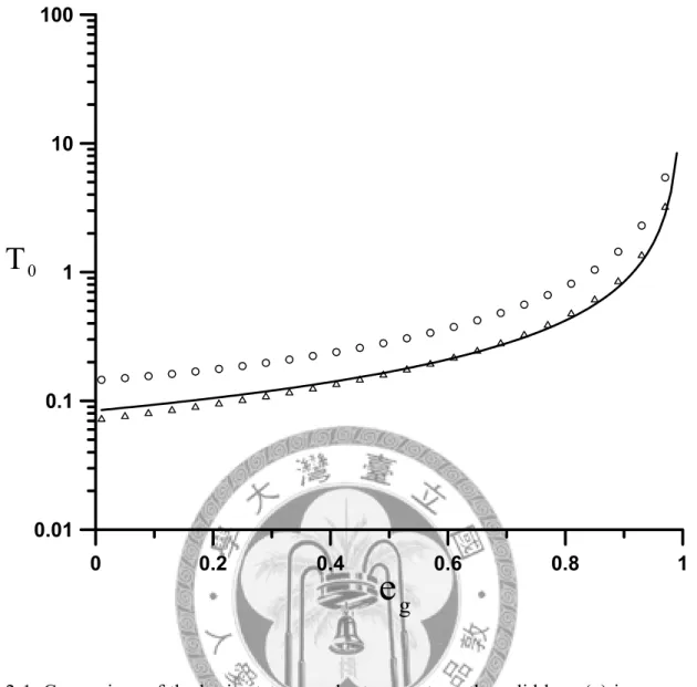
Figure 1-1: Figure 2 of the paper (the A&N 1997). 8 Figure 1-2: Figure 3 of the paper (the A&N 1997). 9 Figure 1-3: Figure 12 of the paper (the A&N 1997). 10 Figure 2-1: Comparison of the basic-state granular temperature, the solid lone

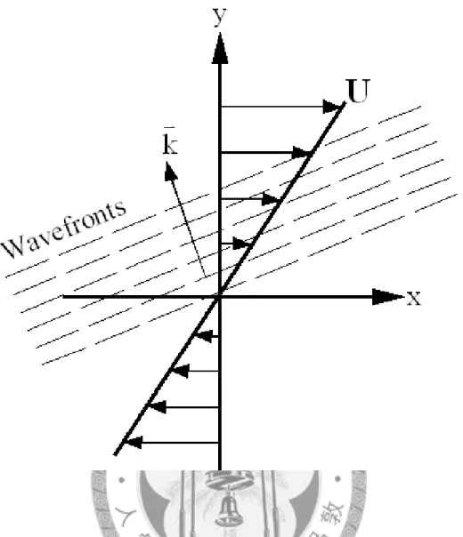
(–) is our result; the circle (○) is for ν₀ =0.2 by the A&N; the triangle (△) is for ν₀ =0.6 by the A&N. 24 Figure 2-2: The Schematic of flow geometry. It illustrates that the mean

velocity profile U(y) which can rotate the direction of disturbance wavenumber vector kv

and wave-fronts. 25

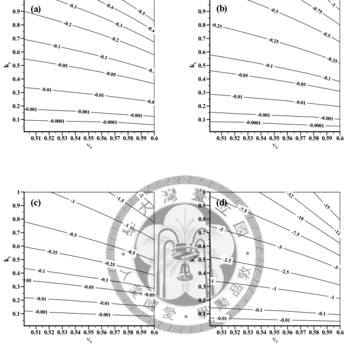
Figure 4-1: Contours of ω_r^l for 0.01≤k_y ≤1 and 0.501≤ν₀ ≤0.6 . The coefficient of restitution e is set as (a) 0.4, (b) 0.6, (c) 0.8 and (d) _g

0.99. 49 Figure 4-2: Contours of ω_r^l. Part (a) is for ν₀ =0.51; (b) for ν₀ =0.55; (c) for

6

0 =0.

ν . 50

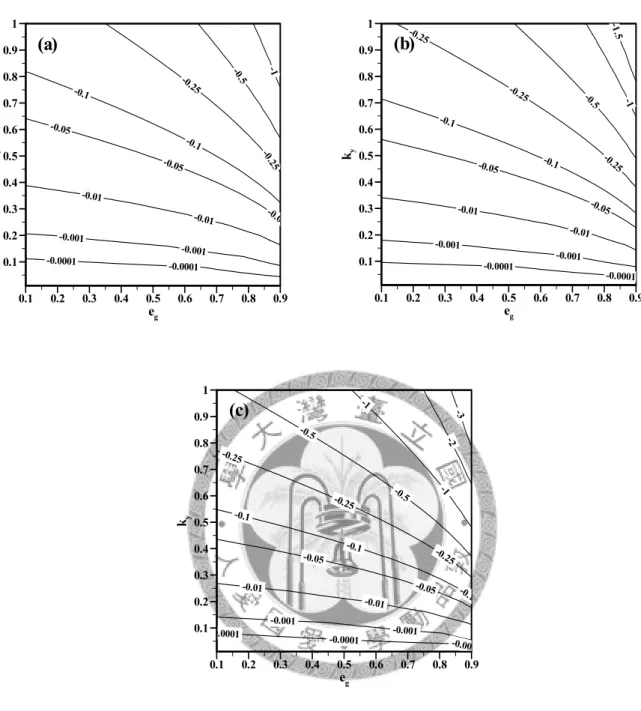
Figure 4-3: Contours of initial transient growth rate Ω_i in the

(

ν₀,ky

)

plane for four cases: (a) e_g =0.2; (b) e_g =0.5 ; (c) e_g =0.8 ; (d)

9 0.

e_g = . 51

Figure 4-4: Contours of initial transient growth rate Ω_i in the

(

eg,ky

)

plane for (a) ν₀ =0.51; (b) ν₀ =0.55; (c) ν₀ =0.6. 52 Figure 4-5: Temporal evolution of transient growth function G(t) for k_y =1,

8 0.

e_g = and ν₀ =0.55. 53

Figure 4-6: Temporal evolution of G(t) for k_y =0.05, where parts of (a) and (b) are decomposed for short-term and long-term scale, respectively.

Other parameters are set the same as those of Figure 4-5. 54 Figure 4-7: The temporal development of each component. Part (a) is for the

contribution of density; (b) for the contribution of kinetic energy;

(c) for the contribution of random fluctuation. Other parameters are

consistent with those of Figure 4-5. 55

Figure 4-8: The temporal development of each component for short-term. All the parameters are consistent with those of Figure 4-6. 56 Figure 4-9: The temporal development of each component for long-term of

Figure 4-8. 57

Figure 4-10: The temporal development of each component. Other parameters for (a)–(c) are the same as those of Figure 4-5. 58 Figure 4-11: The temporal development of each component. Other parameters

for (a)–(c) are specified as those of Figure 4-5. 59 Figure 4-12: Contours of maximum transient growth G_max in the

(

ν₀,ky

)

plane

for four cases: (a) e_g =0.2 ; (b) e_g =0.5 ; (c) e_g =0.8 ; (d) 9

0.

e_g = . 60

Figure 4-13: Contours of the time T in the _max

(

ν₀,ky

)

plane. Parts of (a)–(d) and other parameters are the same as those of Figure 4-12. 61 Figure 4-14: Contours of product by Ω_i and T_max in the

(

ν₀,ky

)

plane for

8 0.

e_g = . 62

Figure 4-15: Contours of initial transient growth rate Ω_i for non-layering modes in the

(

kx,ky

)

plane, where ν₀ =0.55. Part (a) is for

2 0.

e_g = ; (b) for e_g =0.5; (c) for e_g =0.8; (d) for e_g =0.9. 63 Figure 4-16: Contours of initial transient growth rate Ω_i for non-layering

modes in the

(

ν₀,ky

)

plane and the value of k is set to 0.5. Other _x parameters of (a)–(d) are specified as those of Figure 4-15. 64 Figure 4-17: Contours of initial transient growth rate Ω_i for non-layering

modes in the

(

ν₀,ky

)

plane and the value of k is set to 0.1. Other _x parameters for (a)–(d) are the same as those of Figure 4-15. 65 Figure 4-18: Temporal evolution of G(t) for (a) k_x =1 and (b) k_x =0.1. Other

parameters are set as k_y =1, 55ν₀ =0. and e_g =0.5. 66 Figure 4-19: Temporal evolution of G(t) for ν₀ =0.6. Other parameters are

consistent with those of Figure 4-18. 67

Figure 4-20: Temporal evolution of G(t) for e_g =0.8. Other parameters are

consistent with those of Figure 4-18. 68

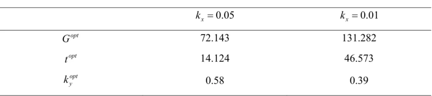
Figure 4-21: Variation of maximum transient growth G_max with k . The solid _y line is for k_x =0.01 and the dashed line for k_x =0.05, where the parameters are set as e_g =0.5 and ν₀ =0.55. 69 Figure 4-22: Temporal evolution of the optimal growth function G for (a) ^opt

05 0.

k_x = and (b) k_x =0.01. 70

Figure 4-23: The temporal evolution of each component from G^opt for 05

0.

k_x = . 71

Figure 4-24: The distribution of solids volume fraction disturbances for two cases: (a) t=0 and (b)t^opt =14.124. Parameters are set as k_x =0.05,

58 0.

k_y^opt = , 55ν₀ =0. and e_g =0.55. 72 Figure 4-25: Asymptotic contours of ω_r^l for the case of adding quasi-static

stresses. Parameters are set as N=0.001 and e_g =0.5. Most the values of ω_r^l are about to −10⁻¹⁴~−10⁻¹⁵. 73

Table list

Table 2-1: Constitutive parameters 12

Table 2-2: Non-dimensional functions 23

Table 4-1: Values of G_max and t for different parameters _0.1 e and _g ν₀ (k_y =1) 38 Table 4-2: Values of G , ^opt t and ^opt k^opt_y for two different 46

Symbols

11 1~ A

A Non-dimensional functions

C Velocity fluctuation

c Instantaneous velocity of single particle

d Diameter

e g Coefficient of restitution

( )

ν

g Radial distribution function

( )

t

G Transient growth function

Gmax Maximum transient growth

G opt Optimal transient growth

k x Streamwise wavenumber

k y Initial transversal wavenumber

opt

ky Optimal initial transversal wavenumber ]

[M System matrix

[ ]

M _L Matrix of layering modes

N Reference value of P_f

P Mean pressure

P c Collisional pressure

P f Frictional pressure

[Q(t)] Fundamental matrix

( )

t

R_ν Contribution of density

( )

t

R_KE Contribution of kinetic energy

( )

t

R_T Contribution of random fluctuation

t Time

1 .

t 0 Decayed time

tmax Maximum time

t opt Optimal time

T The granular temperature

u Streamwise mean velocity

v Transversal mean velocity

ν Solids volume fraction

νmin Minimum solids volume fraction

νmax Maximum solids volume fraction

ρ Bulk density

ρs Density of individual particle

σij Surface stress tensor

δij Kronecker delta

γ_& ij Rate of deformation tensor

μ Shear viscosity

λ Bulk viscosity

κ Conductivity

Φ Energy dissipation

qv Energy flux

−1

Γ Time scale

( )

t

χ^v Solution of disturbance amplitude

χv 0 Initial condition

ηv i Eigenvectors of

[ ]

^M _L

ωi Eigenvalue of

[ ]

M _L

l

ωr Real part of the least-stable eigenvalue

[Λ ] Diagonal matrix

εmax Maximum eigenvalue of

[ ] [ ]

Q^H Q Ωi Initial transient growth rate

⋅ Bulk average

( )

⋅ ^∗ Dimensional variable

( )

⋅ ₀ Basic-state variable

( )

⋅ ^′ Perturbation variable

( )

⋅~ Amplitude variable

⋅ 2-norm

Chapter 1 Introduction

1.1 Motivation

Granular materials have received significant attention to numerous scientific studies and industrial applications during the past two decades. Granular flows are the continuous deformation of granular medium which is composed of solid particles. The motion of one solid particle can be predicted precisely by Newton second law. However, when particles gather considerably, the behavior of particles become very difficult and complicated to explain. Consequently, various theories have been studied to explain the behavior of a granular flow. The gas like behavior of dilute or moderate granular flows has been studied by gas kinetic theory, which leads to current granular flow kinetic theory. Then the early granular kinetic theory was established by replacing gas molecules with grains. To correspond with practical granular matter, the grains have been considered as inelastic matter so that energy dissipation due to collisions of particles cannot be neglected. According to the gas kinetic theory, the granular flows were assumed to rapid deformation and lower density. At low solids volume fraction, numerous constitutive theories have been proposed to describe rapid granular flows. There are mainly two theories which have been widely applied to various dilute state problems. One is proposed by Lun et al. (1984) and by Jenkins

& Richman (1985). Both are based on the gas kinetic theory. The above two models deemed that granular particles interact through uncorrelated instantaneous binary collisions at low solids volume fraction. According to the above two models, considerable researches have predicted several physical features successfully. However, one special limiting case of granular flows is the quasi-static regime which represents the higher solids volume fraction and slower deformation.

Then the mechanism of a dense granular flow is very different from rapid granular flows. The stress

in the quasi-state regime should be considered not only due to repeated collisions but also frictional contacts among dense particles. Today, the theories of rapid granular flows have been developed.

Dense granular flows still lack a unified constitutive theory, because granular materials can behave like a solid, liquid, or gas. In the next subsection, we will introduce some significant constitutive models for dilute and dense granular flows.

1.2 Literature survey

Granular materials have been used for numerous scientific and industrial applications, which include mineral, powder, ceramic-process, rockfalls, avalanches, pack-ice, debris flows, and granular lubrication (Takahashi 1981; Campbell et al. 1995; Iverson 1997; Andreotti et al. 2002;

Bounhoure et al. 2002; Aranson & Tsimring 2006; Emmanuel et al. 2007). It is still a matter of debate of the effect of shear strain rates and solids volume fraction. According to the behavior of granular medium, granular flows can be divided into three regimes and two of them have achieved significant success in numerous studies and applications. One is the quasi-static regime which possesses the characteristics of slow deformation and high concentration. This regime has widely developed in the soil-mechanics. The other is the rapid flow regime which possesses the contrary characteristics － fast deformation and low concentration to those of the quasi-static regime. Both the quasi-static regime and rapid flow regime belong to dense and dilute state, respectively. The above two regimes are important, but the third occurs in an intermediate, transitional flow regime that lies between the above two regimes. Savage (1998 & 2008) has proposed revised constitutive equations which based on the theories (Lun et al. 1984; Jenkins & Richman 1985). Those two equations are kinetic-theory-based constitutive equations (KTBCE, thereinafter) describing dry monodisperse dense cohesionless granular flows in which the pressure is composed of strain-rate-independent frictional stress and rate-dependent collisional stresses.

We introduce the collisional stress firstly. As mentioned in the last subsection, the collisional stress is in analogy with gas pressure which is caused through the impacts among molecules. By the definition of granular material, there are two different points from the gas kinetic theory: (1) solid particles except instantaneous collisional effect, a force can be transmitted by long-term contract; (2) since the collision between naturally inelastic particles, certain energy will be lost during impact collisions. Thus, three important physical factors can influence collisions. They are solids volume fraction, the coefficient of restitution and the granular temperature. The range of the coefficient of restitution is from the nearly elastic (0.9) to the extremely dissipative value (0.1). The solids volume fraction is defined by the ratio of the occupied volume by particles to entire volume. The large magnitude of solids volume fraction can cause the collective behavior which a large number of inelastic collisions occur among particles. This inelastic property of granular collisions cause granular clustering within a granular flow. Granular clustering has first been proposed by Hopkins

& Louge (1991) and the effect of clustering has induced the distribution of stress and changed the behavior of granular rheology for any flow geometry. Therefore, the collisional stress can be defined by the combination of solids volume fraction and coefficient of restitution, and the effect of the random motion of the particles should be considered. According to the kinetic theory of gas, grains are continuous and fluctuating within a granular flow. Because the time of collisional contact approaches zero and only binary collisions occur, this chaotic random motion exists approximate to one at low or moderate concentration. The random fluctuation of grains can be characterized by means of a statistical velocity distribution function. Then the random velocity distribution function can be established by the Maxwell’s assumptions: (1) the distribution of granular velocities is independent of time at any spatial location; (2) the random velocity components are statistically independent after a large number of collisions; (3) the distribution does not have preferred direction and is independent of the orientation of the coordinate system; (4) when two spheres collide, the direction after collision is distributed with equal probability. In this thesis, we use the radial

distribution function g(ν) of the papers (Johnson & Jackson 1987; Nott & Jackson 1992; Alam &

Nott 1997), g(ν) is approximate to one at low concentration but increases with increasing concentration. This function describes the probability of finding two particles in close proximity and prevents over-compaction of granular matter between grains when they are close to each other.

The function g(ν) depends only on solids volume fraction and we will show g(ν) in the next chapter. In order to more precisely define the random fluctuating motion of grains in granular flows, a significant physical factor of the granular temperature is considered. From the view point of dynamic, the granular temperature is associated with ensemble concept of individual translational velocity fluctuation of individual particles. The velocity fluctuation is defined by C =c-u, where c is the instantaneous velocity of single particle and u= c is defined as the bulk average velocity of whole particles. The symbol of brackets denotes as an ensemble average. Then the velocity fluctuation C is also treated as the velocity of the fluctuation motion of grains. Therefore, the granular temperature is defined by T ≡ C² /3 which can be an index that measures the velocity of the random motion. The granular temperature can be viewed as a fluctuating energy per unit of mass of granular flows (3T 2). The granular temperature is caused by the granular shear work and decreases through the inelastic collision. Hence, the loss of granular energy due to inelastic collision is referred to as energy dissipation, which causes a transformation of granular temperature to conventional heat temperature. According to the above fundamental factors, the granular collisional stress can be established by combining those factors together.

At higher solids volume fraction, because grains experience long-term contracts during rubbing and rolling on each other, collisions should not be treated as instantaneous one. Because a kinetic theory model is not accurate to describe the stress at higher concentration, a frictional stress should be taken into consideration. To deal with the mechanics at dense state, the Mohr-Coulomb law has

which will be sheared when the shear stress reaches its critical value. This critical magnitude can be referred as the onset of yielding which asserts that a granular material will yield by shearing.

According to the Mohr-Coulomb law, the behavior of material will be rigid and does not experience any strain rate as the below line. When the shear stress increases to the yield line, this onset point means that the material will go into the plastic state. Because the Mohr-Coulomb law cannot accurately describe the behaviors of flowing and deforming above the yield line, therefore, the expression of stress should be considered the kinematics of granular motion after yielding. The plastic potential theory has been brought up, which can be allied with the Mohr-Coulomb law successfully and provide a way to predict the velocity distribution within the granular medium at yield. Then the plastic potential theory connects stress and velocity gradient. Since the shear viscosity and bulk viscosity are not constant coefficient parameters, they are elaborate functions of velocity gradient. Additional important phenomenon is that the density will change at initial plastic state. This phenomenon may be referred to as the dilatancy or consolidation by the decreasing or increasing density. Then the yielding behavior based on the Mohr-Coulomb law should be revised by considering for the above two phenomena. Hence, the yield locus is established and the critical state is defined as zero derivative of the yield locus curve. When the critical state occurs, the variation of bulk density cease and the granular materials deform without any change of its volume.

Thus, the plastic potential theory and the critical state model can be combined with the flow rule to establish the frictional stress.

According to the above introduction of collisional stress and frictional stress, the presented paper (Savage 1998; Savage 2008) in which the frictional stress is expressed by a log function of the solids volume fraction (Savage 1998) and by fractional form (Savage 2008). In this thesis, we use the latter form of frictional stress which can be increased by the larger solids volume fraction and diverge as the solids volume fraction attains to the maximum value. Hence, we can obtain both the

quasi-static and collisional stresses which are all dependent on solids volume fraction, and then the frictional stress is independent of shear strain rate. Recently, a visco-plastic model has been derived from the discrete simulation of dense plane-shear flows of disks. Visco-plastic model proposes that shear stress is composed of yielding stress and collisional stress. Following this model, the study (G.

D. R. Midi. 2004) presented that an onset shear stress is needed for overcoming the yielding stress in various configurations. Then Jop et al. (2006) proposed a new visco-plastic constitutive equation for dense granular flows and the constitutive equation is dependent on the experimental parameter (inertial number), where the effective friction coefficient is measured as function of the inertial number comparable to experimental data. Because the visco-plastic model is a phenomenological model, this model lacks of the physical parameters such as the coefficient of restitution and the granular temperature. Thus we do not use this model in this study. In this thesis, we use the same constitutive equations derived in the paper by Savage (2008) to compare the results with other constitutive equations (Alam & Nott 1997) for the unbounded uniform dense granular shear flows (UUDGSF, thereinafter) problem. Alam & Nott (1997) (A&N, thereinafter) proposed a different way from Savage to describe the frictional stress of a dense granular flow. The A&N considered that the frictional stress is added to the momentum equation but Savage (2008) included frictional stress into mean pressure. Because the paper (Hopkins & Louge 1991) observed that the effect of clustering of increased particle concentration, might cause that the initially uniform random distribution of particles were unstable under shear. The stability problem for the unbounded uniform granular shear flows has been researched in several papers (Savage 1992; Babic 1993; Schmid &

Kytomaa 1994; Wang et al. 1996). The method of stability analysis is based on the eigenvalue technique for asymptotic results, and the other way is to observe whether the system is stable by 2-norm operator for transient analysis. Those two methods will be introduced in the Chapter 3. Next, we will list the related equations and figures which are derived from the A&N (1997) and Savage (2008). First, we show Eq. (10) and (12) of Savage (2008) as follows

⎥⎦

⎢ ⎤

⎣

⎡ ⎟

⎠

⎜ ⎞

⎝⎛ + +

+

= π ρσ π

μ 1 ¹²

5 4 16 1 5 6

2

1 G

T G (1-1)

and

⎥⎦

⎢ ⎤

⎣

⎡ ⎟

⎠

⎜ ⎞

⎝⎛ + +

+

= π ρσ π

κ 9

1 32 5 6 24 1 5 16

15 ₁₂ G

T G , (1-2)

where all parameters of above two equations are defined in the paper (Savage 2008).

Then we show Eq. (5.7) – (5.10) of the A&N (1997) as follows )

0 ( )

( ν

ν′ t = ′ , (1-3)

( )

t u

( ) ( )

u t

u′ = ′ 0 −υ′ 0 ⁰_y , (1-4)

( )

υ

( )

0

υ′ t = ′ , (1-5)

and

( )

t T

( )

0e ^β2t ν (0)

(

1 e ^β2t

)

β1 β2

T′ = ′ ⁻ + ′ − ⁻ , (1-6)

where all parameters of above four equations are defined in the paper (the A&N 1997). Then we show three figures of the A&N (1997) in the following. These figures are often used to compare with our results. There are Figure 2, Figure 3 and Figure 12 of the A&N (1997).

1.3 Organization of thesis

This thesis applies the linear stability analysis for the dense unbounded granular shear flows in two dimensional problems. In Chapter 1, we describe the background of granular flow and the objects of this context. In Chapter 2, we derive a basic-state solution and two dimensional perturbation equations of the constitutive equations (Savage 2008). In Chapter 3, we firstly introduce the criterion of stability for different analyses in every subsection and then discuss the asymptotic and transient results for different wave structures. We will make conclusions and give some advices for future research in Chapter 4. Other information is presented in the appendix.

Figure 1-1. Figure 2 of the paper (the A&N 1997).

Figure 1-2. Figure 3 of the paper (the A&N 1997).

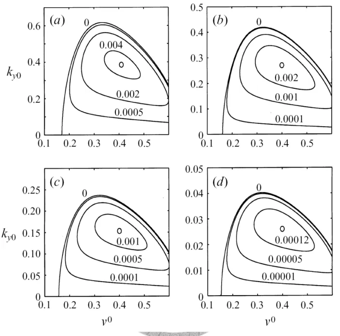
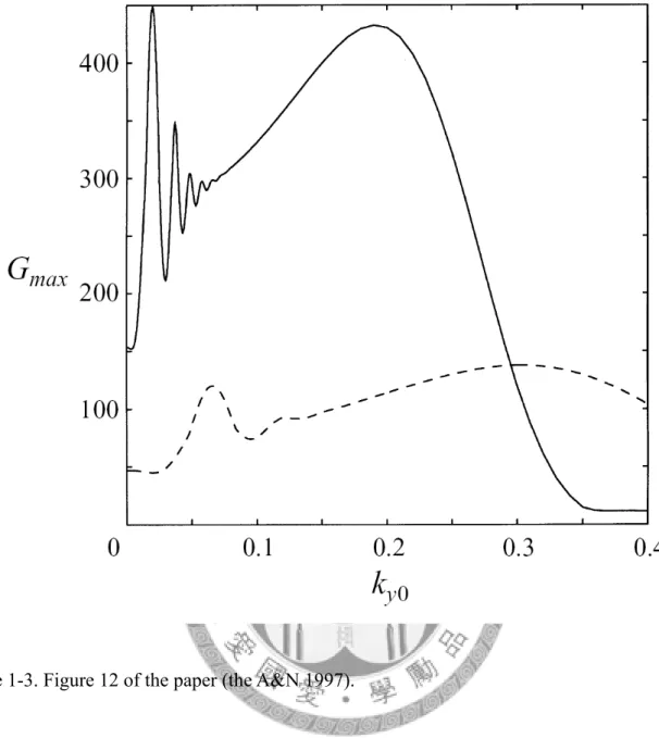
Figure 1-3. Figure 12 of the paper (the A&N 1997).

Chapter 2

Mathematical model

This thesis is to apply revised granular flows kinetic theory (Jenkins & Richman 1985) by Savage (2008) to study two dimensional stability analysis. The constitutive equations are modified by adding an additional term to the pressure. This additional term is referred to as the quasi-static contribution. However, the A&N (1997) directly added the frictional contribution to the momentum equation for dense granular flows. We examine the UUDGSF using inelastic identical spherical particles. The relative motion of two plates will generate a shear onto the entire dense particles to move in the x -direction. To simplify the problem, we neglect the effect of the body force term in ^∗ the momentum equation and focus on two dimensional granular flows problem.

2.1 Governing and constitutive equations

We begin by applying the results of governing and constitutive equations which were formulated by Savage (2008) for identical spherical smooth inelastic particles. The conservation of mass, momentum and fluctuation kinetic energy are given by

=0

∂ ρ +∂

∂ ρ +∂

∂ ρ

∂

∗

∗

∗

∗

∗

∗

∗

∗

y v x

u

t , (2-1)

∗ ∗

∗

∗

∗

∗

∗ ∗ ⎟⎟⎠=∇ ⋅

⎜⎜ ⎞

⎝

⎛ + ⋅∇

∂

∂ σ

ρ u u

t

uv v v

, (2-2)

and

∗

∗

∗

∗

∗ ∗

∗

∗ ∗

∗

∗ ∗

∗

∗ ∗ ⎟⎟= ⋅∇ −∇ ⋅ −

⎠

⎜⎜ ⎞

⎝

⎛

∂ + ∂

∂ + ∂

∂

∂ σ Φ

ρ u q

y v T x u T t

T v v

2

3 , (2-3)

where the superscript “∗ ”denotes dimensional lengths, time, mean velocities and stresses in Eq.

(2-1)–(2-3) and afterward. In the above Eq. (2-1)–(2-3), where ρ^∗ is the bulk density which

depends on the density of individual particle ρ_s^∗ and solids volume fraction ν , t the time, ^∗ uv ^∗ the mean velocity vector ^{uv∗ =}

(

^u∗,v∗

)

^{, σ∗} the symmetric surface stress tensor; T the granular ^∗ temperature, qv the flux of particle fluctuation energy vector and ^∗ Φ^∗ the rate of energy dissipation per unit volume. The symmetric surface stress tensor is given by

∗

∗

∗

∗

∗

∗

∗ = − + ∇ ⋅ _ij + _ij

ij P λ u δ μ γ

σ ( v ) _& . (2-4)

The first term of the right hand side of above equation is the mean pressure. In the Savage’s studies (1998 & 2008), he considered the normal stresses which are induced by collisional and quasi-static contributions simultaneously. Collisional stress occurs in the assumption of kinetic theory model － instantaneous binary particle collisions. Yet in the dense granular flows regime, particles exist long-term frictional and rubbing contact, this result is defined as the quasi-static stress. In this reason, we name the frictional term of mean pressure as P_f^∗ for the quasi-static contribution and

the collisional term of mean pressure as P for the collisional contribution. The mean pressure is _c^∗ composed of the summation of the above two contributions which are shown as

( )

( )

^{∗ ∗}

∗

∗

∗

∗ +

−

= − +

=P P N gT

P _{f c} ρν

ν ν

ν ν

β α

4

max

min , (2-5)

where N is the reference value of ^∗ P_f^∗ according to the paper (Savage 2008), ν_max the maximum solids volume fraction, ν_min the minimum solids volume fraction, α and β the integers which are widely used in the papers (Johnson et al. 1990 ; Nott & Jackson 1992). Above parameters are listed in Table 2-1.

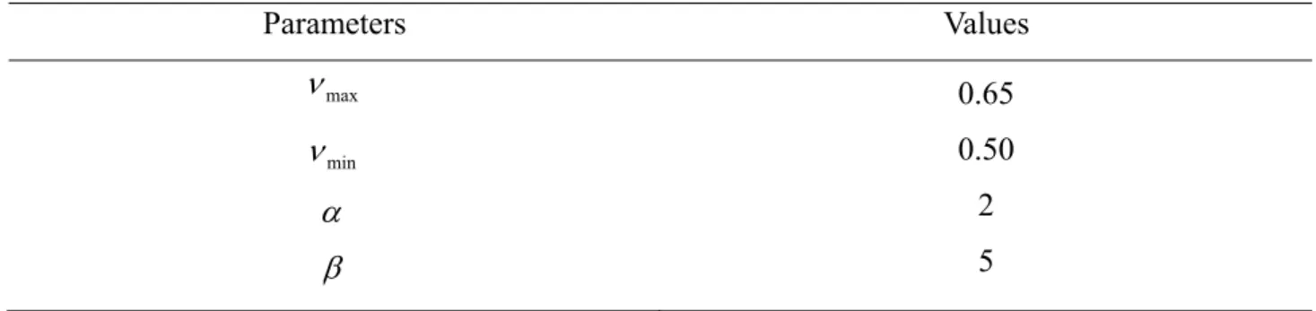
Table 2-1: Constitutive parameters

Parameters Values νmax

ν min

α β

0.65 0.50 2 5

The dimensionless function of g

( )

ν is the radial distribution function. The radial distribution function has been introduced in last chapter and this function expresses collisional stress which varies with the solid volume fraction. In this study, we use the same form of g

( )

ν of Savage (2008), it is given by

( )

1

(

_max

)

¹³

1 ν ν ν

= −

= g

g , (2-6)

The equation of Eq. (2-6) is limited solids volume fraction ν to less than a maximum value ν_max. It ensures that the stress will diverge as the solid fraction approaches to the closest state, thus preventing solid fraction from an unphysical large value. The second term of the right hand side of Eq. (2-4) is the bulk viscosity which is given by

( )

¹²

3 2

∗

∗

∗ = ∗

T P d

λ π . (2-7)

The third term of the right hand side of Eq. (2-4) is the shear viscosity and the shear strain rate tensor, respectively, which are shown as

( )

^{⎜⎝⎛ + ⎟⎠⎞}

= ∗

∗

∗ ∗

1 12 5

2

2 1

π μ π

T P

d (2-8)

and

∗

∗

∗

∗ ∗

∂ +∂

∂

= ∂

i j j ij i

x u x

γ_& u , (2-9)

where γ_&ij^∗ denotes the rate of deformation tensor of the velocity field.

And the energy flux vector is composed of conductivity and gradient of T which is given by ^∗

∗

∗

∗

∗ =− ∇T

q^v κ , (2-10)

where the conductivity is

( )

^{⎜⎝⎛ + ⎟⎠⎞}

= ^∗_∗ ^∗

∗

32 1 9

2 1

π κ π

T P

d . (2-11)

The collisional rate of energy dissipation per unit volume is

2

) 1

1 (

6 ⎟⎟⎠

⎜⎜ ⎞

⎝

− ⎛

= _∗ ^∗

∗

∗

Φ ^Tπ

d P e_g

, (2-12)

where e is the generalized coefficient of restitution for the spherical particles (cf. Savage 2008). _g As we can see, Eq. (2-8) and Eq. (2-11) are very different from the original forms Eq. (1-1) and Eq.

(1-2). In order to satisfy dense, high concentration granular flows, kinetic terms of Eq. (1-1) and (1-2) of Savage are negligible and these expressions can be transformed into approximate forms. To correspond with approximate results, we restrict the range of ν is about 0.5 ~ 0.6. The equations of Eq. (2-7), Eq. (2-8), Eq. (2-11) and Eq. (2-12) are the properties of granular flows. All of them are mainly composed of the mean pressure and the granular temperature. Because the mean pressure which possesses frictional and kinetic contributions in different concentration, these equations of Eq. (2-7), Eq. (2-8), Eq. (2-11) and Eq. (2-12) can be influenced by various density state.

2.2 Basic-state derivation and non-dimensional process

2.2.1 Basic-state derivation

Before obtaining the linear perturbation equations, we should establish the basic-state solutions.

We assume that the steady =0

∂

⋅

∂

t∗ and fully-developed =0

∂

⋅

∂

x∗ basic conditions are used to apply the unbounded uniform shear configuration in x -direction with constant velocity. The basic-state ^∗ solutions are obtained

0^∗ =0

v , (2-13)

∗

P is uniform, 0

∂ =

∂

∗

∗

y u₀

constant value, (2-14)

⎥⎥

⎥⎥

⎦

⎤

⎢⎢

⎢⎢

⎣

⎡

∂

∂

∂

∂

=

∗

∗

∗

∗

∗

0 0

0 0

0 ,

y u

y u γ_&ij ,

and

(2-15)

( )

2 0 2

0 151

1 12 ) (

⎟⎟⎠

⎜⎜ ⎞

⎝

⎛

∂

∂

−

⎟⎠

⎜ ⎞

⎝⎛ +

= _∗^∗

∗

∗

y u e

d T

g

π

, (2-16)

where the subscript “0” is applied throughout the thesis to denote a basic state variable thereafter.

Almost above equations are uniform values except the basic-state granular temperature which depends only on the coefficient of restitutione . _g

2.2.2 Non-dimensional process

We use the diameter of individual particle d as the length scale and the inverse of shear strain ^∗ rate Γ^∗−1 as time scale for the unbounded uniform shear problem. We list essential dimensionless variables as follows, they are lengths, time, velocity, pressure and granular temperature, respectively,

( )

⁼ _∗

(

^{x∗ y∗}

)

y d

x 1 ,

, ,

∗

= ∗t

t Γ ,

∗

∗

= ∗ u

uv d v

Γ

1 ,

(

^{∗ ∗}

)

^∗

= ∗ P

P d

s

2

1 Γ

ρ ^,

and

( )

^{Γ∗ ∗ ∗}

= T

T d1 ₂ .

Then the dimensionless conservation of mass, momentum and energy equations are shown in sequence as follows

( )

⁼⁰

⋅

∇

∂ +

∂ u

t

νv

ν , (2-17)

σ

ν ⎟=∇⋅

⎠

⎜ ⎞

⎝

⎛ + ⋅∇

∂

∂ u u

t

uv v v

, and

(2-18)

Φ σ

ν ⎟⎟⎠= ⋅∇ −∇⋅ −

⎜⎜ ⎞

⎝

⎛

∂ + ∂

∂ + ∂

∂

∂ u q

y v T x u T t

T v v

2

3 . (2-19)

After conducting the non-dimensional process, Eq. (2-4), Eq. (2-5), Eq. (2-7)–(2-12) are shown in the dimensionless form as follows

ij ij

ij P λ u δ μγ

σ =(− + ∇⋅^v) + _& , (2-20)

( )

( )

^gT

N P P

P _{f c} ²

max

min 4ν

ν ν

ν ν

β α +

−

= − +

= , (2-21)

( )

¹²

3 2

T P

λ = π , (2-22)

( )

^⎟⎠

⎜ ⎞

⎝⎛ +

= 1 12

5 2

2 1

π μ π

T

P (2-23)

i j j i

ij x

u x u

∂ +∂

∂

= ∂

γ_& , (2-24)

T

q^v=−κ∇ , (2-25)

( )

^⎟⎠

⎜ ⎞

⎝⎛ +

= 32

1 9

2 1

π κ π

T

P ,

and

(2-26)

(

^eg

)

^{T P}

2 1

1

6 ⎟

⎠

⎜ ⎞

⎝

− ⎛

= π

Φ . (2-27)

Basic-state variables Eq. (2-15) and Eq. (2-16) can also be set to the non-dimensional form, such that are given by

⎥⎦

⎢ ⎤

⎣

=⎡ 0 1

1 0

0 ,

γ_&ij _(2-28)

and

(

eg

)

T −

⎟⎠

⎜ ⎞

⎝⎛ +

=151 1 12

0

π .

(2-29) The equation of Eq. (2-29) is the dimensionless basic-state granular temperature which is only dependent on the coefficient of restitution. It is different result of the paper (cf. p.273 of the A&N 1997) and our Eq. (2-29), because the A&N presented that the basic-state granular temperature depends both on solids volume fraction and the coefficient of restitution. In spite of the fact that the granular temperature is dominated by different physical variables, the evidenced values of the granular temperature are drawn in Figure 2-1. Figure 2-1 indicates that the tendency of the granular temperature from different forms is obviously agreement. In this study, we restrict the range of e _g from 0.1 to 0.9 and the range of T will correspond to 0.093 ~ 0.841. ₀

2.3 Linear perturbation process

We apply the first-order perturbed variables to the original basic-state variables in the two dimensional problem. We list unknown variables which are solid volume fraction, velocity vector and granular temperature, respectively,

(

x ,,y t

)

0 ν

ν

ν = + ′ , (2-30)

( )

u v

(

u u

(

x y t

)

v v

(

x y t

) )

uv = , = ₀+ ′ , , , ₀+ ′ , , ,

and (2-31)

(

x y t

)

T T

T = ₀+ ′ , , , (2-32)

where the superscript symbol of primed quantities are applied throughout the thesis to denote the

infinitesimal disturbances. The disturbed variables depend on two-dimensional spatial and temporal variables. The radial distribution function Eq. (2-6) can be derived to the basic state and the perturbed state:

( ) ( ) ( )

( )

(

⁻

)

^{⎜⎜⎝⎛ ′ ⎟⎟⎠⎞}

− +

′ = +

= − + ′

=

0 3 2 1 max 0

3 1 max 0 3

1 max 0 3

1 max 0

0 1 1 3

1 1

1

ν ν ν

ν ν ν ν

ν ν

ν g ν

g

g . (2-33)

The first term of right hand side of above Eq. (2-33) is the basic-state radial distribution function

(

_{0 max}

)

¹³

0 1

1 ν ν

= −

g , (2-34)

and the second term is the disturbed radial distribution function

ν ν

ν ν

ν ν

ν

= ′

⎟⎟

⎠

⎞

⎜⎜

⎝

⎛

⎟⎟⎠

⎜⎜ ⎞

⎝

−⎛

⎟⎟⎠

⎜⎜ ⎞

⎝

⎟⎟ ⎛ ′

⎠

⎜⎜ ⎞

⎝

⎛

′= _{2 0}² ₁

3 1

max 0

0 3 1

max 0

1 3 1

A g

g ,

and A₁is applied to simplify the complicated disturbed form and shown as follows

(2-35)

3 2

0 3 1

max 1

1 1

3

1 ⎟⎟⎠

⎜⎜ ⎞

⎝

⎟⎟ ⎛

⎠

⎜⎜ ⎞

⎝

= ⎛

ν

A ν . (2-36)

The first part of mean pressure Eq. (2-21) is the frictional contribution, the basic state and perturbed state of frictional pressure P_f can be derived as follows

( )

( ) ( )

( ) ( )

(

^{νν νν}

)

^ν

ν β ν ν

ν ν α ν

ν ν ν

β α β

α β

α ′

− + −

− ′ + −

−

= − + ′

= ⁻ ₊₁

0 max

min 0 0

max

1 min 0 0

max min 0 0

, P N N N

P

P_{f f f} . (2-37)

According to the above equation of Eq. (2-37), we can obtain the basic state and disturbed state of frictional pressure, respectively,

( )

( )

^β

α

ν ν

ν ν

0 max

min 0 0

, −

= N −

P_f ,

and

(2-38)

( )

( ) ( )

(

ν ν

)

^{ν ν}

ν ν ν β

ν ν

ν ν α

β α β

α ′= ′

− + −

− ′

= −

′ ⁻ _{+1 ,0 2}

0 max

min 0 0

max

1 min

0 N P A

N

P_{f f} , (2-39)

where A₂is applied for the reason of brevity Eq. (2-39) and A₂ can be written as

0 max min 0

2 ν ν

β ν

ν α

+ −

= −

A . (2-40)

Then the other part of mean pressure Eq. (2-21) is the collisional contribution, the basic state and disturbed state of collisional pressure can also be derived as

T g g

T T

g T

g P

P

P_c = _c,0+ _c′=4ν₀² _{0 0}+8ν_{0 0 0}ν′+4ν₀² ₀ ′+4ν₀² ₀ ′. (2-41) The first part of right hand side of Eq. (2-41) is the basic-state collisional pressure

0 0 2 0 0

, 4 g T

P_c = ν (2-42)

and the others are the disturbed collisional pressure T

g T

A g T

g

P_c′=8ν_{0 0 0}ν′+4ν₀² ₀² _{1 0}ν′+4ν₀² ₀ ′. (2-43) Hence, we can include the above two parts into the mean pressure. We show the basic-state mean pressure firstly

0 0 2 0 0

max min 0 0

, 0 ,

0 P P N 4 g T

P _{f c} ν

ν ν

ν

ν ₊

⎟⎟⎠

⎜⎜ ⎞

⎝

⎛

−

= − +

= , (2-44)

and disturbed mean pressure

T g A

T g T

A g T

g A

P P P

P′= _f′ + _c′= _{f,0 2}ν′+8ν_{0 0 0}ν′+4ν₀² ₀² _{1 0}ν′+4ν₀² ₀ ′= ₃ν′+4ν₀² ₀ ′, (2-45) where A is composed of ₃ A₁ and A₂

0 0 0 0 1 2 0 2 0 2 0 ,

3 P A 4 g AT 8 g T

A = _f + ν + ν . (2-46)

Then we apply similar derived process to the rest variables and obtain the basic-state and disturbed variables individually. First, we list the basic-state variables as follows

( )

^⎟⎠

⎜ ⎞

⎝⎛ +

= 1 12

5 2

2 1 0

0 0

π μ π

T

P , (2-47)

( )

₀⁰¹²

0 3 T

2P

λ = π , (2-48)

( )

^⎟⎠

⎜ ⎞

⎝⎛ +

= 32

1 9 T

P

2 1 0

0 π

κ₀ π ,

(2-49)

( )

0

2 1

0 61 T0 P

e_g ⎟

⎠

⎜ ⎞

⎝

− ⎛

= π

Φ ,

and

(2-50)

⎥⎦

⎢ ⎤

⎣

⎡

−

= −

0 0

0 0

0 P

P μ

σ μ . (2-51)

And then the disturbed variables are listed as follows

⎥⎥

⎥⎥

⎦

⎤

⎢⎢

⎢⎢

⎣

⎡

∂

∂ ′

∂

∂ ′

∂ +

∂ ′ ∂

∂ ′

∂ +

∂ ′

∂

∂ ′

′ =

y v x

v y u

x v y u x

u

ij 2

2

γ_& ,

(2-52)

( ) ( ) ( )

T ^{A AT}

T P T

P ⎟= ′+ ′

⎠

⎜ ⎞

⎝⎛ +

− ′

⎟⎠

⎜ ⎞

⎝⎛ +

= ′

′ _{32 4 5}

0 2 1

0 2

1

0 1 12

12 5 5 1

2 π ν

π π

μ π ,

(2-53)

( )

3

( ) ( )

T ^{A AT}

T P T

3 P

7 2 6

3 0 2 1

0 2

1 0

+ ′

= ′

− ′

= ′

′ ν

π

λ π² ,

(2-54)

( ) ( ) ( )

T ^{1 932 A AT} T

P 32

1 9 T

P

9 0 8

2 1 0

+ ′

= ′

⎟⎠

⎜ ⎞

⎝⎛ +

− ′

⎟⎠

⎜ ⎞

⎝⎛ +

= ′

′ π ν

π π

κ π ₃₂

0 2

2 1 ,

(2-55)

( ) ( )

( )

T ^{T A A T} P

P e

e_g T − ^g ′= ₁₀ ′+ ₁₁ ′

′+

⎟⎠

⎜ ⎞

⎝

− ⎛

′= ν

π Φ π

0 0 2

1

0 31

1

6 ,

and

(2-56)

⎥⎥

⎥⎥

⎦

⎤

⎢⎢

⎢⎢

⎣

⎡

∂

∂ ′

⎟⎟+

⎠

⎜⎜ ⎞

⎝

⎛

∂

∂ ′

∂ +

∂ ′

′+

⎟⎟ −

⎠

⎜⎜ ⎞

⎝

⎛

∂

∂ ′

∂ +

∂ ′

′+

⎟⎟⎠

⎜⎜ ⎞

⎝

⎛

∂

∂ ′

∂ +

∂ ′

′+

∂

∂ ′

⎟⎟+

⎠

⎜⎜ ⎞

⎝

⎛

∂

∂ ′

∂ +

∂ ′

′+

−

′=

y v y

v x P u

x v y u

x v y u x

u y

v x P u

0 0

0

0 0

0

2 2

μ λ

μ μ

μ μ μ

λ

σ . (2-57)

Because the above disturbed variables are too complicate to read, we can use several dimensionless variables to simplify the original forms. All the parameters are listed in Table 2-2. In the last