福山地區維管束附生植物之物種組成及功能性狀在垂直方向的變化趨勢

(1)

doi: 10.6342/NTU201900489

國立臺灣大學生農學院森林環境暨資源學系碩士論文

School of Forestry and Resource Conservation College of Bioresources and Agriculture

National Taiwan University Master Thesis

福山地區維管束附生植物之物種組成及功能性狀在垂直方向的變化趨勢

Species Composition and Functional Traits of Vascular Epiphytes Show Vertical Trends in

Fushan Experimental Forest

李先祐 Hsien-Yu Lee

指導教授：李靜峯博士及丁宗蘇博士

Advisor: Ching-Feng Li, Ph.D. & Tzung-Su Ding, Ph.D.

中華民國 108 年 2 月 February, 2019

(2)

doi: 10.6342/NTU201900489

i

口試委員會審定書

(3)

doi: 10.6342/NTU201900489

ii

謝辭

兩年半的時間匆匆而過，不知不覺間這篇碩士論文也即將要完成了，回想起來還真覺得有些不可思議。以前看別人的論文謝辭，總會覺得何必列這麼多名字。但等到自己真正開始做研究，才知道需要感謝的人真的太多了！

首先要感謝丁宗蘇老師，在我對研究題目還完全沒有頭緒的時候就願意收留我，而且很有耐心地陪我摸索研究的方向。在換過好幾次題目，也嘗過幾次挫敗之後，終於能夠完成這個我覺得有趣的研究題目，真的非常感謝老師耐心的指導。感謝五木老師願意指導我植群研究的方法。當初決定要做附生植物之後，因為自己並沒有扎實的植群研究基礎，內心實在沒有把握，但得知五木老師願意指導後就安心許多。何其有幸能擁有兩位這麼好的指導老師，希望我沒有辜負你們的期望。

I have to thank Professor David Zelený for giving many suggestions about

sampling methods, statistical analyses (especially community weighted mean analysis) and thesis structure. I also need to thank you for sharing your laboratory and measuring instruments with me. Although your name is not on the cover of my thesis, you are just like an advisor to me. 感謝徐嘉君老師願意擔任我的口試委員並給予我很多建議。

徐老師是附生植物研究的翹楚，真的很榮幸這篇論文能通過您的審核。感謝建融學長，當我還在摸索研究方向時就願意帶著我在福山探索，給我很多想法上的啟發，之後也一直不辭辛勞協助我在福山的研究工作。野外研究有時難免會碰到一些危險，多虧有建融學長才讓我度過重重難關。真的非常感謝學長，抱歉給學長添了不少麻煩。

感謝 401 的大家，奕全學長在我初期嘗試做聲景研究時幫我很多忙。阿明學姊一直都很可靠，關於推甄、研究、寫論文和口試的事情都給我很多建議。立中和光平常常在 meeting 時提出一針見血的問題。芷怡、佳祈、芳伃也都有在 meeting 或口試的時候幫我忙。雖然我不常待在研究室，但我真的很喜歡 401 的

(4)

doi: 10.6342/NTU201900489

iii

氣氛，很高興這兩年半能在這裡度過。感謝植群研究室和生態復育研究室的各位，這裡的 meeting 讓我收穫很多。特別感謝宗儀，在我研究初期給我很多有用的建議，第一次調查時還特地騎車來福山一趟，在蕨類物種的辨識上也幫了很多忙。也要感謝信彥幫我辨識很多我認不出來的樣本。

感謝所有辛苦幫我做野外採樣以及室內量測工作的夥伴，煒杰、建匡、安雅、可風、聿筠、育任、智翔、亦欣、亭羽、彥喬、亮廷、毓蓉、是奎，沒有你們我應該很難撐過這些枯燥的工作。我在研究期間的運勢好像不太好，不但碰到強烈寒流，還有被虎頭蜂攻擊跟發生車禍，對於那些被我的厄運波及的夥伴我也要再說一次抱歉。感謝俊佑學長以及福山研究中心的各位給我很多幫助。感謝何傳愷老師願意出借葉綠素計和硬度計給我使用，也感謝欣怡學姐和正涵的幫忙。

最後要感謝我的家人，在密集收資料和寫論文的期間我真的很少回家，連跨年的連假和春假也都跑去收資料了，回家的次數甚至快要比在日本念書的姐姐還少，

真的感謝大家的體諒。

一篇論文的完成，除了需要一個研究生鍥而不捨的拚搏，還需要無數人從旁協助。感謝所有幫助我完成這篇論文的人。

(5)

doi: 10.6342/NTU201900489

iv

中文摘要

在森林中包括光度、相對濕度及溫度等環境因子都會隨高度改變，形成垂直的環境梯度。維管束附生植物因為生長在其他植物之上，面對從林下層到樹冠層的多樣微環境，因此適合用來研究垂直環境梯度對生物的影響。本研究針對在臺灣東北部福山試驗林的附生植物，以釐清附生植物的物種組成以及功能性狀是否會隨著高度改變。本研究選定 24 棵樣樹，在每棵樣樹上劃設 5-6 個垂直分區，並透過雙索攀樹技術，在各分區內設立樣區進行物種調查。除了記錄樣區內的物種及豐度，

亦採集個體量測功能性狀，包括葉厚度、比葉面積、葉乾物質重、單位葉面積葉含水率以及葉綠素含量 (單位葉面積及單位葉質量) 。

研究結果顯示，樣區的物種組成會隨離地高度而改變。各物種會佔據不同的高度範圍，形成垂直分層分布。此外，對於單葉的附生植物物種來說，葉厚度以及單位葉面積葉含水率會隨高度上升而增加，比葉面積和單位葉質量的葉綠素含量則會隨高度上升而減少。本研究指出離地高度確實對附生植物的分布以及功能性狀都具有顯著的影響。

【中文關鍵字】

維管束附生植物、垂直環境梯度、垂直分層分布、功能性狀、群落加權平均

(6)

doi: 10.6342/NTU201900489

v

Abstract

Vascular epiphytes grow on other plants, facing various micro-environments from dark and humid understory to bright and dry canopy. Therefore, it is quite suitable to use epiphytes to analyze the effects of vertical environmental gradients on organisms. I studied vascular epiphytes in Fushan Experimental Forest (located in northeastern Taiwan) in 2018 and aimed to determine whether species composition and several functional leaf traits of vascular epiphytes change along vertical environmental gradients. I used doubled rope techniques to climb up 24 sampled trees and surveyed the epiphytes on them. I set 5-6 vertical zones within each sampled tree based on height above ground, and set sampling plots within each zone, recorded all species that appeared in the plots and their abundance. I also collected some epiphyte individuals to measure functional traits including leaf thickness, specific leaf area, leaf dry matter content, leaf water content (per unit area) and leaf chlorophyll content (per unit area and per unit mass).

The results show that epiphyte species composition changed significantly with height, and epiphyte species differentiated in their height distribution. Angle differences between aspects of plots and the south direction were also suggested to have effects on epiphyte species composition. Besides, several functional leaf traits show vertical trends.

Leaf thickness and leaf water content (per unit area) of simple-leaved epiphytes significantly increased with height, while specific leaf area and chlorophyll content (per

(7)

doi: 10.6342/NTU201900489

vi

unit mass) decreased with height. This study reveals that height is an important factor which not only structures species composition but also creates vertical trends of several functional leaf traits.

Keywords

Vascular epiphytes, vertical environmental gradients, vertical stratification, functional traits, community weighted mean

(8)

doi: 10.6342/NTU201900489

vii

List of Figures

Figure 1. Common vertical environmental gradients in forests ... 6

Figure 2. Three types of filtering mechanisms ... 8

Figure 3. Filtering mechanisms, species composition and the niche concept ... 10

Figure 4. A trait-height relationship and underlining mechanisms ... 15

Figure 5. The location of Fushan Experimental Forest ... 19

Figure 6. A HOBO data logger hung on the trunk ... 21

Figure 7. Ambient temperature variations within a day of positions at different heights ... 22

Figure 8. Relative humidity variations within a day of positions at different heights ... 23

Figure 9. Daily mean values and standard deviation (SD) of ambient temperature and relative humidity (RH) at different heights ... 24

Figure 10. The locations of sampled trees ... 26

Figure 11. Vertical zones of a sampled tree ... 28

Figure 12. A sampling plot used to survey epiphytes ... 29

Figure 13. Positional variables recorded for each plot ... 30

Figure 14. Leaf-scanning procedures ... 35

Figure 15. Plots below and not below bird’s-nest ferns in DCA space ... 40

Figure 16. Number of plots in different vertical zones ... 41

Figure 17. Definition of two positional variables calculated from aspect ... 43

Figure 18. Negative correlation between height and diameter of substrate ... 44

Figure 19. Epiphytic types and taxonomy groups of abundant epiphyte species ... 46

Figure 20. Result of the PCA on mean trait values of 25 epiphyte species ... 50

Figure 21. Two approaches used to analyze relationships between functional traits and positional variables ... 54

(11)

doi: 10.6342/NTU201900489

x

Figure 22. DCA analysis on plots not below bird’s-nest ferns (showing plots) ... 57

Figure 23. DCA analysis on plots not below bird’s-nest ferns (showing species) ... 58

Figure 24. Optimal CCA model using two explanatory variables ... 60

Figure 25. Height distribution of the 23 abundant epiphyte species ... 62

Figure 26. Relative frequency in each vertical zone for four species ... 64

Figure 27. ADS distribution of the 23 abundant epiphyte species ... 65

Figure 28. Relationships between functional traits and all positional variables based on individual-based linear model ... 67

Figure 29. Scatterplots showing relationships between individual-based functional traits and height ... 68

Figure 30. Relationships between all positional variables and functional traits based on plot-based CWM analysis ... 70

Figure 31. Scatterplots showing relationships between CWM trait values and height .. 71

Figure 32. Johansson’s zoning scheme ... 78

(12)

doi: 10.6342/NTU201900489

xi

List of Tables

Table 1. Six functional traits used in data analyses ... 37 Table 2. Positional variables and the proportion of variation they explained alone in

CCA ... 59 Table 3. The synoptic table showing representative species in each vertical zone ... 63

(13)

doi: 10.6342/NTU201900489

1

Introduction

1. Vascular epiphytes and their importance

Epiphytes are those plants that germinate and grow on other plants (i.e., host plants) without taking nourishments from them (de Mirbel, 1815; Zotz, 2016). In other words, they are not parasitic and can survive on photosynthesis by their own. In a taxonomic perspective, epiphytes can be classified as vascular epiphytes and non-vascular epiphytes.

Vascular epiphytes include those epiphytic species belonging to ferns, fern allies, basal angiosperms, monocots and eudicots, while non-vascular epiphytes refer to epiphytic lichens, mosses and liverworts. Due to large differences between the morphology, physiology, life history characteristics and adaptive strategies of vascular and non- vascular epiphytes, these two types of epiphytes are usually studied separately (Affeld et al., 2008). In this study, only vascular epiphytes were considered. All of the terms

“epiphytes” used in this study refer to vascular epiphytes unless there is an additional

notation.

The definition of epiphytes mentioned in previous paragraph is quite simple, while it is difficult to apply this simple definition under some circumstances because the life history characteristics and the life forms of plants in real world are much more complicated. Those species of which all individuals are epiphytic and not connected to the ground during all stages of life history belong to epiphytes without question. Actually,

(14)

doi: 10.6342/NTU201900489

2

these species are also called “true epiphytes” or “holoepiphytes” (Kress, 1989; 徐嘉君, 2007). On the other hand, hemiepiphytes refer to those species which have connections to the ground at some of their life history stages, and can be further classified as primary hemiepiphytes and secondary hemiepiphytes (Kress, 1989). Primary hemiepiphytes grow on other plants during early stages but finally reach the ground and become terrestrial plants, such as some Ficus species. Secondary hemiepiphytes germinate from the soil, but they lose the connection to the ground sooner or later, such as Pothos chinensis (in Araceae). There are also some species of which some individuals are epiphytic while the

other individuals are terrestrial or lithophytic. These species are usually called

“facultative epiphytes” (Benzing, 2004; Burns, 2010).

True epiphytes, primary and secondary hemiepiphytes and facultative epiphytes were all viewed as epiphytes when Kress (1989) described the systematic distribution of vascular epiphytes in the world. When 徐嘉君 (2007) summarized the species list of vascular epiphytes in Taiwan, she also adopted this general definition. However, there are still some debates about the definition of epiphytes. For example, Zotz (2013) suggested that secondary hemiepiphytes should not be considered as epiphytes because they are quite similar to climbing plants (vines) physiologically. In this study, I used a more general definition of epiphytes like Kress (1989) and 徐嘉君 (2007), that including true

(15)

doi: 10.6342/NTU201900489

3

epiphytes, primary and secondary hemiepiphytes, and facultative epiphytes, while excluding accidental epiphytes and climbing plants.

According to Zotz (2013), there were 27614 species of vascular epiphytes in the

world, approximately equaling to 9% of all vascular plant species. At a local perspective, this proportion (also called “epiphyte quotient”) may be even higher. In some tropical

montane cloud forests, epiphytes may account for up to 30% of all vascular plant species (Küper et al., 2004). For such high proportions, it seems that epiphytes should not be ignored when studying regional or local plant communities. However, due to the paucity of efficient methods to reach forest canopies, not much emphasis were put on epiphytes in canopies until 1980s (Lowman et al., 2012), causing a research gap that should be filled.

Vegetation ecologists have observed and surveyed terrestrial plants for a long time.

However, it seems that the principles summarized from these studies cannot be applied to epiphyte assemblages directly (Zotz, 2016). For example, interspecific competition and herbivory are important factors shaping the structures and dynamics of tree communities, while their influences on epiphytes are much more subtle (Zotz and Hietz, 2001). The three-dimensional distribution patterns of epiphytes are also quite different from the planar distribution of terrestrial plants. Hence, there is a need to study the vegetation structure of epiphytes.

(16)

doi: 10.6342/NTU201900489

4

In Taiwan, the epiphyte quotient is about 8% (徐嘉君，2007), slightly less than epiphyte quotient in the world (9%). Although there are many studies on epiphytes in tropical regions, especially in Central and South America, epiphytes in subtropical and temperate regions get less attention (Zotz, 2016). Studies on epiphytes of Taiwan can fill this research gap.

2. Environmental gradients that epiphytes experience

Large scale environmental gradients such as latitudinal or elevational gradients may have some effects on the distribution or diversity of epiphytes. For example, species richness of epiphytic ferns declines from tropical to temperate regions, and the trend is much sharper than terrestrial ferns (Zotz, 2016). It is also suggested that the abundance and species richness of epiphytes are hump-shaped distributed along elevational gradient, reaching maximum values in cloud forest zone which is typically at intermediate elevation (e.g., Krömer et al., 2005).

At a local scale, epiphytes may also experience various microenvironments.

Growing on other plants, epiphytes are actually distributed in a three-dimensional space, and the microenvironments may change a lot in both horizontal and vertical directions.

In horizontal direction, there are many factors that may influence microenvironments, causing complicated structures. For example, the distance to forest edge (Davies-Colley

(17)

doi: 10.6342/NTU201900489

5

et al., 2000), the distance to water source (Chilpa-Galván et al., 2013), the position along

the slope (Werner et al., 2012) all have effects on microenvironments and may hence influence epiphyte assemblages.

On the other hand, the environmental gradients along vertical direction are much more stable and predictable. Solar radiation is suggested to decline dramatically from outer canopy to understory (Petter et al., 2016). In a lowland forest in Panama, the mean daily illuminance at 20 m high was about 22% of the illuminance in outer canopy, and the ratio dropped to only 6% in understory layer (Wagner et al., 2013). In other tropical forests, the ratio of illuminance in understory relative to that in outer canopy may be even lower (Richards, 1996). Air humidity also changes along vertical direction, which becomes higher and more stable from outer canopy to understory (Wagner et al., 2013).

It should be noticed that both vertical light and humidity gradients only exist during daytime. Illuminance and air humidity have been suggested to have nearly no difference between understory and canopy during night (Wagner et al., 2013; Zotz, 2016). There is also a pronounced vertical temperature gradient, but this gradient is more complicated.

Temperature may increase, decrease or nearly not change from understory to canopy, depending on season or time in a day (Christy, 1952). However, daily temperature fluctuation is typically larger in higher places (Wagner et al., 2013). Besides, wind speed usually increases from understory to outer canopy (Oliver, 1971), and diameter, stability

(18)

doi: 10.6342/NTU201900489

6

and longevity of growing substrates (trunks, branches and twigs) also change along vertical direction (Cabral et al., 2015).

In summary, many environmental variables, including solar radiation, air humidity, temperature fluctuation and wind speed, all change along vertical direction (Figure 1).

What effects these vertical environmental gradients have on vascular epiphyte assemblages is the main question that this study was aimed to answer.

Figure 1. Common vertical environmental gradients in forests

Light intensity, temperature fluctuation and wind speed typically increase with height, while air humidity and diameter of growing substrates (trunks or branches) decrease with height. (modified from Petter et al., 2016)

(19)

doi: 10.6342/NTU201900489

7

3. Effects of vertical environmental gradients on species composition

Explaining species composition of local communities is a central theme in ecology

(Weiher and Keddy, 1995). A set of species which may potentially colonize a site is usually called the “species pool” of that site (Pärtel et al., 2011), and several mechanisms

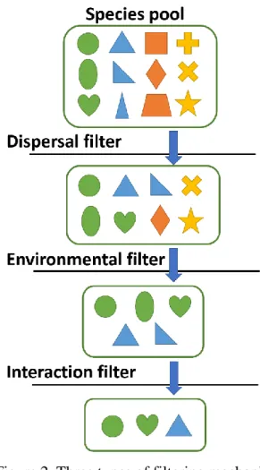
have been proposed to filter a species pool into observed species composition of a local community. Three types of filtering mechanisms are usually mentioned, including dispersal filter, abiotic environmental filter and biotic interaction filter (Cadotte and Tucker, 2017) (Figure 2). Dispersal filter first excludes those species unable to arrive at the site due to limitations of dispersal abilities. Environmental filter excludes those species not capable of establishing and persisting in such environmental conditions (Bazzaz, 1991), and biotic interactions such as competition and predation may furthermore filter out some species (Hardy et al., 2012). Although these three types of filtering mechanisms are usually described as sequential and discrete processes, they actually interact with each other in complex ways in reality (Cadotte and Tucker, 2017).

(20)

doi: 10.6342/NTU201900489

8

Figure 2. Three types of filtering mechanisms

These three types of filtering mechanisms were proposed to explain species composition of a local community. Each symbol in this figure represents a species within species pool of the community. Dispersal filter excludes those species cannot disperse to the site, environmental filter excludes those species cannot persist in that abiotic environment, and interaction filter excludes those species cannot persist because of biotic interactions like competition. (modified from Cadotte and Tucker, 2017)

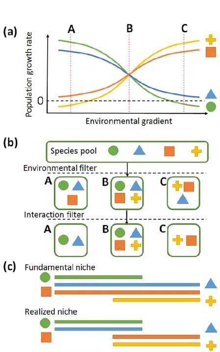
These filtering mechanisms can also be applied to several local communities distributed along an environmental gradient. In this case, environmental filter is usually considered most influential (Kraft et al., 2015). For gradual change of environmental conditions, the set of species which can pass environmental filter also changes. As a result,

(21)

doi: 10.6342/NTU201900489

9

a sequential change of species composition along the environmental gradient is expected (Laliberté et al., 2014). Besides directly filtering out those species not able to persist, the environmental gradient may also indirectly influence species composition by their effects on biotic interactions. For example, competition ability of a species usually change along the environmental gradient, and a species may be absent in a local community not because of failure to survive in that abiotic environmental condition but because of lower competition ability relative to other coexisting species (Cadotte and Tucker, 2017) (Figure 3a & 3b).

The concept of these filtering mechanisms were proposed to explain species composition of local communities, while they can be linked to the niche concept of species. Hutchinson (1957) described the fundamental niche of a species as a state of

abiotic environment which permits that species to exist, and can be viewed as an “n- dimensional hypervolume” of which each dimension represent one environmental

variable. However, he also pointed out that a species usually only utilize a subset of its

fundamental niche because of biotic interactions, and this subset was called “realized niche”. From this point of view, environmental filter actually filter out those species

whose fundamental niche do not encompass the environmental condition of the site, so environmental filter is also called a “niche-based” process (Püttker et al., 2015). The other way around, the distribution range of a species after considering the effects of

(22)

doi: 10.6342/NTU201900489

10

environmental filter reflects its fundamental niche, and the distribution range reflects its realized niche after considering the effects of both environmental and biotic interaction filter (Figure 3c).

Figure 3. Filtering mechanisms, species composition and the niche concept

(a) Population growth rate of a species can reflect its fitness or competition ability, and usually change along environmental gradients. Four symbols showed in the right

(23)

doi: 10.6342/NTU201900489

11

represent four different species. A, B and C represent three communities located along this environmental gradient. If population growth rate is less than 0 (below black dash line), that species cannot persist in that environment even if there is no competitor. (b) Species composition in three communities (A,B and C) are determined by both environmental and interaction filters. The environmental filter excludes those species with population growth rate less than 0 (e.g. yellow cross species in community A), while the interaction filter excludes those species with population growth rate larger than 0 but not large enough to compete with other species (e.g. orange square species in community A). (c) Distribution range of a species after considering environmental filter reflects its fundamental niche, while the range after considering both environmental and interaction filters reflect its realized niche. (partly modified from Cadotte and Tucker, 2017)

As mentioned in previous section, solar radiation, air humidity, temperature fluctuation and wind speed all change along vertical direction in a forest. All of these environmental variables are influential to physiology of plants. For example, net primary productivity of a leaf usually increases with the amount of photosynthetically active radiation (PAR) received until reaching saturation (Ö gren and Evans, 1993). Air humidity directly influences vapor pressure deficit between a leaf and the air, and hence has strong effects on transpiration rate (Lambers, 2008). A moderate increase in temperature usually causes an increase in primary productivity (Sage and Kubien, 2007), while usually accompanied by increasing vapor pressure deficit and transpiration rate (Lambers, 2008).

Therefore, these vertical environmental gradients are expected to have strong direct or

(24)

doi: 10.6342/NTU201900489

12

indirect effects on species composition. A sequential change of species composition along these gradients as well as a differentiation of niches occupied by each species are expected as a result.

Many previous studies have reported that different epiphyte species occupied

different height ranges on host trees just as the expectation above, and this phenomenon was called “vertical stratification” (Johansson, 1974; Nieder et al., 2000; Krömer et al.,

2007; Zotz, 2007; Parra et al., 2009). However, most of these studies were done in tropical forests, especially in Central and South America. Whether vertical stratification of epiphyte species also exists in subtropical forest in Taiwan is one of the questions that this study was aimed to answer.

4. Effects of vertical environmental gradients on functional traits

Functional traits are measurable attributes of an organism, which strongly influence its performance or fitness (McGill et al., 2006). These attributes may be morphological, physiological, biochemical, phenological or behavioral (Violle et al., 2007). Functional traits usually reflect how organisms respond to environments, that is, their adaptive strategies (Nock et al., 2016).

Analyzing the relationships between functional traits and environmental gradients can be helpful to better understand the mechanisms structuring communities (Ackerly and

(25)

doi: 10.6342/NTU201900489

13

Cornwell, 2007; Petter et al., 2016). As mentioned in previous section, environmental gradients may cause a change in species composition by direct or indirect effects.

However, competition alone or even stochastic process may also lead to similar patterns even if environmental gradients have no effect on performances of species (Kraft et al., 2015). Hence, it is difficult to infer the influences of environmental gradients simply by observed patterns of species composition. Functional traits, on the other hand, can reveal more information about how organisms respond to environments. Therefore, if a change in species composition is accompanied by strong relationships between functional traits and environmental gradients, it is suggested with more confidence that this change was caused, at least partly, by environmental gradients (Cadotte and Tucker, 2017). Besides, analysis of functional traits can also reveal potential trade-offs when organisms adapt to environments (Wright et al., 2004; Gotsch et al., 2015).

For vascular epiphytes, the ratio of leaf mass to whole plant mass are usually high (Zotz and Asshoff, 2010), so leaf traits received more attention in previous studies (Petter et al., 2016). Several functional leaf traits are suggested to reflect how plants adapt to

environments with different levels of solar radiation or moisture, and hence are expected to change along vertical environmental gradients in forests. For example, specific leaf area (SLA), defined as leaf area divided by leaf dry mass, is related to light-capturing efficiency, and tends to be larger in shaded understory environment (Wright et al., 2004).

(26)

doi: 10.6342/NTU201900489

14

Leaf thickness (LT), on the other hand, is predicted to be larger in sunnier and drier environments to reduce water loss by transpiration and prevent overheating (Pérez- Harguindeguy et al., 2016). Other leaf traits such as leaf dry matter content, leaf water content (per unit area) and leaf chlorophyll content (per unit area or per unit mass) are also expected to change along vertical environmental gradients (Petter et al., 2016).

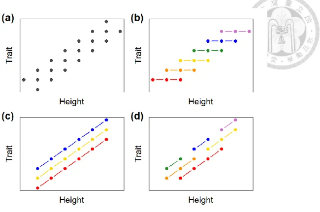
If a functional trait of all epiphyte individuals in a site is observed to change along vertical direction, this changing pattern may come from two different mechanisms. The first one is species turnover along vertical gradients, and the other is change in functional trait value along vertical gradients within each species (i.e., intraspecific trait variation) (Cornwell and Ackerly, 2009). These two mechanisms may work alone or work together, and give rise to very similar patterns (Figure 4). In order to determine what mechanism causes observed pattern, a further analysis of intraspecific trait variation is necessary.

Although vertical stratification of epiphytes were frequently reported, few studies have analyzed functional traits of epiphytes (see Cavaleri et al., 2010 and Petter et al., 2016). This study was aimed to analyze the relationships between several leaf functional traits of all epiphytes and vertical environmental gradients, and also tried to figure out whether these relationships exist within each species.

(27)

doi: 10.6342/NTU201900489

15

Figure 4. A trait-height relationship and underlining mechanisms

(a) Trait values of individuals are observed to change with height. (b) This pattern may be caused by species turnover alone. (Each color in the figure represents one species.) (c) This pattern may be caused by intraspecific trait variation alone. (d) This pattern may also be caused by both species turnover and intraspecific trait variation.

(28)

doi: 10.6342/NTU201900489

16

5. Purposes of this study

From the introduction in previous sections, there are obvious vertical environmental gradients within forests, and these gradients are expected to have effects on both species composition and functional traits of vascular epiphytes. Therefore, this study was aimed to:

(1) determine whether height is an important factor that influences epiphyte species composition, and identify other significant factors;

(2) describe the vertical distribution patterns of different epiphyte species in the study area;

(3) examine the trends of functional leaf traits of all epiphytes with height and other factors;

(4) determine whether functional leaf traits of individuals of the same epiphyte species change significantly with height.

(29)

doi: 10.6342/NTU201900489

17

Methods

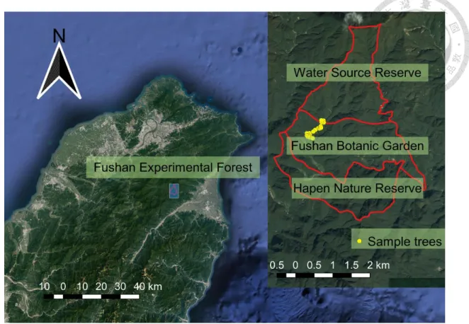
1. Study site

This study was conducted in Fushan Experimental Forest which is located in northeastern Taiwan, just at the border between New Taipei City and Yilan County (Figure 5). Fushan Experimental Forest belongs to the north part of Snow Mountain Range geographically. The altitude range is from 400 m to 1400 m. It belongs to Northeastern Inland Climate Zone defined by 蘇鴻傑 (1985) or Montane Subtropical Wet-Hot-Summered Climate Zone defined by 梁玉琦 (2004). This type of climate zone is characterized by high precipitation during the whole year, with nearly no dry season.

According to weather data collected by two weather stations (Fushan Nursery Weather Station and Hapen Weather Station) located within the study site during 1988 to 2011, the mean annual temperature was about 18.4 °C, and annual precipitation was 3787.3 mm.

There were 206 rainy days per year on average, and mean annual relative humidity could be as high as 93.3 %, supporting that this area is rainy and humid all year round (陸象豫及黃惠雪，2013) and hence providing ideal weather for epiphytes to grow.

The natural vegetation in Fushan Experimental Forest belongs to Machilus- Castanopsis belt defined by 蘇鴻傑 (1984) or Machilus-Castanopsis type defined by

林建融 (2009). Dominant tree species in this vegetation type include species of

Lauraceae, Fagaceae and Theaceae. Based on previous surveys, there are more than 200

(30)

doi: 10.6342/NTU201900489

18

species of vascular epiphytes in Fushan Experimental Forest, account for more than half of the vascular epiphyte species in Taiwan (徐嘉君，2013). However, a strong cold air mass passed through Fushan Experimental Forest in January 2016, and several vascular epiphyte species, especially epiphytic orchids, were killed by cold weather (林建融，

personal communication).

Fushan Experimental Forest was divided into three districts—Water Source Reserve, Fushan Botanic Garden and Hapen Nature Reserve from north to south (Figure 5). Most of the sampled trees surveyed in this study were located in Fushan Botanic Garden, while the others were within Water Source Reserve. However, all of them were within the same watershed (Hapen Creek Watershed).

(31)

doi: 10.6342/NTU201900489

19

Figure 5. The location of Fushan Experimental Forest

Fushan Experimental Forest was located in northeastern Taiwan, and it was divided into three districts—Water Source Reserve, Fushan Botanic Garden and Hapen Nature Reserve. Most of the sampled trees surveyed in this study were within Fushan Botanic Garden, while the others were within Water Source Reserve. (The background images of this figure were obtained from Google, 2018)

(32)

doi: 10.6342/NTU201900489

20

2. Vertical environmental gradients within the study site

As mentioned in the introduction, many environmental variables including are suggested to change along vertical direction. In order to confirm vertical environmental gradients in the study site, I used HOBO MX2301 data loggers (Onset Computer Corporation, Bourne, MA, USA) to measure temperature and relative humidity at different height in the forest.

One erect big tree (sampled tree T010) with closed surrounding canopy was selected to hang the HOBO data loggers. I considered canopy closure because measured data may be biased if the logger is directly exposed to sunlight. Five HOBO data loggers were hung and fixed on the trunk at 1, 3, 5, 7 and 9 m height separately. All of the data loggers were hung at similar aspect of the trunk, with aspect range from 220° to 260°, and they were hung at positions where were seldom directly illuminated by sunlight. I also used a white plastic box to shield each HOBO data logger to prevent strong impact by sunlight, rain or falling debris (Figure 6). From August 22 to September 10 in 2018 (20 days in sum), ambient temperature and relative humidity were measured and recorded every 10 minutes for each HOBO data logger.

(33)

doi: 10.6342/NTU201900489

21

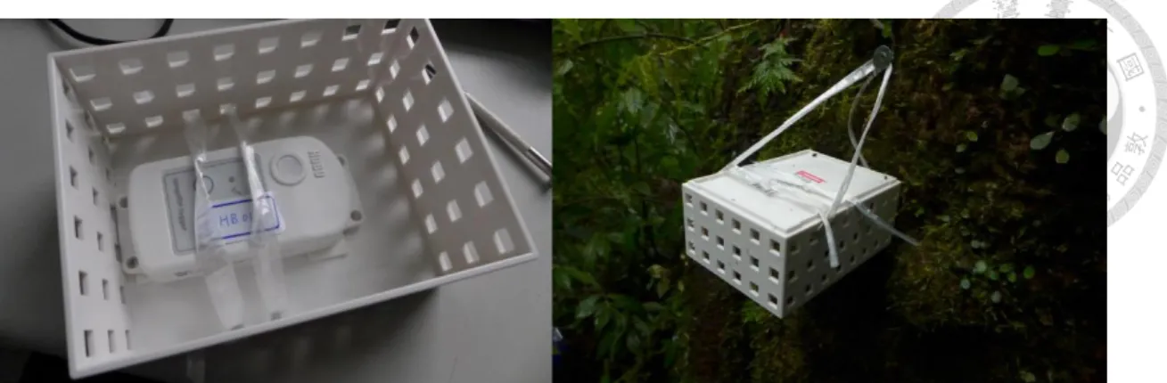
Figure 6. A HOBO data logger hung on the trunk

HOBO MX2301 data loggers were used to measure ambient temperature and relative humidity at different height in this study. The device showed in the left is a HOBO MX2301 data logger. The logger was attached to a white plastic box using double-sided tape and nylon rope, and then was hung on the trunk using screws. The plastic box could protect the logger from direct impact by sunlight, rain or falling debris.

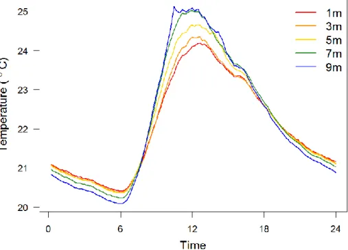
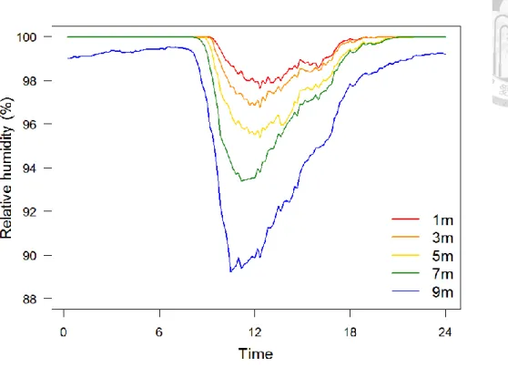
Ambient temperature and relative humidity measurements of the 20 days recording period were averaged and plotted against time of day (Figure 7 and Figure 8). Ambient temperature variation fluctuated widely during the day, lowest around 6 AM and peaked between 12 AM and 1 PM (Figure 7). However, ambient temperature of higher positions was higher than that of lower positions during daytime, especially around noon; but this trend reversed after sunset, temperature of higher positions became lower (Figure 7). This means ambient temperature of higher positions had greater variation within a day, while lower positions had relatively stable ambient temperature. On the other hand, relative humidity showed different patterns (Figure 8). During nights, all positions were quite humid, with relative humidity close to 100%. After sunrise, RH dropped and had obvious

(34)

doi: 10.6342/NTU201900489

22

differences between positions. Higher positions were drier than lower ones during daytime.

Figure 7. Ambient temperature variations within a day of positions at different heights Ambient temperature values showed in the figure are mean values of 20 days. Daily ambient temperature variations of higher positions were larger.

(35)

doi: 10.6342/NTU201900489

23

Figure 8. Relative humidity variations within a day of positions at different heights Relative humidity values showed in the figure are mean values of 20 days. During night, all positions were quite humid, with relative humidity close to 100%, while relative humidity of higher positions became obviously lower during daytime.

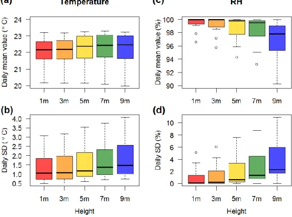
Daily mean values and daily standard deviation (SD) of ambient temperature and relative humidity of each position were calculated, and a nonparametric Friedman test was used to test the differences between positions (setting position as an explanatory variable and date as a block factor). There were no large differences between daily mean temperature values of different positions (Figure 9a). Nonetheless, daily SD of temperature increased significantly with height (Friedman test, p < 0.001) (Figure 9b).

For relative humidity, daily mean values decreased significantly with height (Friedman

(36)

doi: 10.6342/NTU201900489

24

test, p < 0.001) while the SD increased with height (Friedman test, p < 0.001) (Figure 9c

& 9d). The results confirm vertical environmental gradients of ambient temperature and relative humidity existed in the study site. Higher on a tree, environment became drier, and fluctuations of both temperature and relative humidity became more dramatic. This pattern is also consistent to previous studies (Richards, 1996; Wagner et al., 2013).

Figure 9. Daily mean values and standard deviation (SD) of ambient temperature and relative humidity (RH) at different heights

The box plots were drawn based on measurements of a 20-day period. (a) Daily mean ambient temperature didn’t increase or decrease with height. (b) Daily SD of ambient temperature increased with height (Friedman test, p<0.001), indicating larger temperature fluctuations in higher positions. (c) Daily mean relative humidity decreased with height

(37)

doi: 10.6342/NTU201900489

25

(Friedman test, p < 0.001). (d) Daily SD of relative humidity increased with height (Friedman test, p < 0.001), indicating larger relative humidity fluctuations in higher positions.

3. Plot survey for recording epiphyte species

Plot survey method was used in this study to investigate species composition at different microenvironments, as well as the distribution pattern of each species. The first step of survey was choosing sampled trees. Afterwards, I divided each sampled tree into different vertical zones, then set one or more plot(s) within each vertical zone. For each plot, I recorded all plant species appearing inside the plot and their abundance.

There were some considerations when choosing sampled trees. This study mainly focused on the effects of different microenvironments within trees, not the effects of large-scale environmental variables such as elevation or topography. Hence, I selected 24 sampled trees in similar environments. All of them were located in Fushan Botanic Garden and Water Source Reserve, and besides Hapen Creek (Figure 10). The geographic positions and altitudes of these sampled trees were similar. The altitudes of all sampled trees ranged from 600 m to 700 m. The sizes and architectures of trees were also under consideration. Only big canopy trees with heights over 14 m and diameters at breast height (DBH) over 50 cm were chosen (except for sampled tree T003). Besides, all the sampled trees did not incline too much. The inclination angles at breast height were all

(38)

doi: 10.6342/NTU201900489

26

smaller than 20° (inclination angle is 0° if trunk is absolutely erect). To avoid the influences of some tree attributes that related to tree species, only evergreen broad-leaved tree species were chosen. All of the 24 sampled trees belong to Lauraceae except for T023, which belongs to Fagaceae. The detailed information of all sampled trees is shown in Appendix 1.

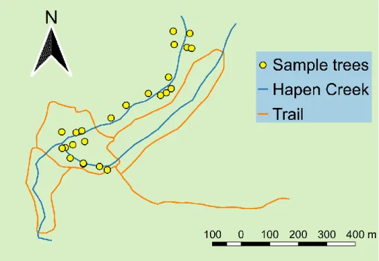
Figure 10. The locations of sampled trees

There were 24 sampled trees in total. All of them were located besides Hapen Creek.

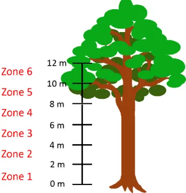
Each sampled tree was divided into several vertical zones based on height above ground, and each vertical zone was 2 m high. Therefore, zone 1 was from the ground to 2 m high, zone 2 was from 2 to 4 m high, and so on (Figure 11). For those vertical zones

(39)

doi: 10.6342/NTU201900489

27

higher than human height, I used doubled rope technique (DdRT) to climb up the tree and survey. The number of vertical zones that could be surveyed depended on accessibility of sampled trees. Therefore, only five vertical zones were surveyed for 18 sampled trees, and only six sampled trees had six vertical zones surveyed.

Within each vertical zone, one or two plot(s) was set to survey epiphytes species composition. When setting a plot, I chose a position where epiphytes species richness was high and the species composition was as representative as possible for that vertical zone.

Each plot was 40×50 cm surface area on trunk or a branch of the sampling tree, and it was further divided into 20 10×10 cm grids. When surveying a plot, all vascular plant species within the plot were recorded as well as the number of grids that each species occupied. The latter was an estimation of species abundance (Figure 12). For all species recorded in the plot, one individual was collected as a voucher which could be used for species identification. Considering accessibility, all of the plots were set on the trunk or erect main branches, not on those branches or twigs growing outward. Some positional variables of each plot were recorded, including the height of plot center, the inclination angle of plot surface, the aspect of the plot relative to the trunk and the dimeter of the growing substrate (the trunk or the branch) (Figure 13). The inclination angle was 0° if the plot was absolutely perpendicular to ground surface. The inclination angle was positive if the plot surface inclined toward the sky, and was negative if inclined toward

(40)

doi: 10.6342/NTU201900489

28

the ground. The aspect of the plot was 0° if the plot set on the north face of the trunk, and ranged from 0° to 359°. These positional variables were used in further analyses.

Figure 11. Vertical zones of a sampled tree

Each vertical zone was 2 m high. Five to six vertical zones were surveyed for each sampled tree.

(41)

doi: 10.6342/NTU201900489

29

Figure 12. A sampling plot used to survey epiphytes

Each plot was 40×50 cm, and it was divided into 20 grids which was 10×10 cm. All vascular plant species within the plot and the number of grids they occupied were recorded. For the case shown here, it is recorded that species A occupies seven grids and species B occupies three grids.

(42)

doi: 10.6342/NTU201900489

30

Figure 13. Positional variables recorded for each plot

Four positional variables were recorded for each plot, including height, inclination angle, aspect and diameter of the growing substrate (the trunk or the branch). Height was the distance between plot center and the ground. Inclination angle was the angle difference between plot surface and vertical direction. Inclination angle was 0° if the plot was absolutely perpendicular to the ground. It was positive if the plot inclined toward the sky, while was negative if the plot inclined toward the ground. Aspect was the angle difference between the direction plot facing and the north direction, ranging from 0° to 359°.

There were some large bird’s-nest ferns growing on trees in the study area. They

actually belonged to two different species, Asplenium antiquum and Asplenium nidus, but sharing quite similar morphology. These bird’s-nest ferns may have some influences on

other epiphytes species, and the species compositions of the places below bird’s-nest ferns were usually different from other places based on observation. Hence, I avoided setting

(43)

doi: 10.6342/NTU201900489

31

plots below bird’s-nest ferns if possible. However, in some vertical zones it was difficult to find a place not influenced by bird’s-nest ferns. For that case, I still set a plot below the bird’s-nest fern, but a special note was taken. There were nine plots below bird’s-nest

ferns in total.

All of the plot surveys in this study were done during January to April, 2018. In total, 24 sampled trees and 139 plots on them were surveyed. There were 52 vascular plant species recorded in these plots, and 39 of them were epiphytes. This study used a general definition of epiphytes, which includes true epiphytes, hemiepiphytes and facultative epiphytes, and life forms of recorded species were determined basically based on the epiphyte species list summarized by 徐嘉君 (2007). The information of all recorded species is shown in Appendix 2.

.

4. Measurements of functional traits

In order to analyze variation of functional traits along micro-environmental gradients, I collected some epiphyte individuals for measurements. There were some criteria when collecting these individuals. First, only mature individuals were collected. Whether an individual was mature or not was judged based on morphology and appearance. For fern species, the existence of reproductive structures (e.g., sori) could be used to judge. The leaves of these individuals should be healthy, not wilted or rolled, and without any spot,

(44)

doi: 10.6342/NTU201900489

32

wound, gall or other signs indicating disease or herbivory. All of the individuals used to measure functional traits were collected from those 24 sampled trees. However, due to the limitation of tree-climbing method, small twigs located away from tree trunks were difficult to access. Therefore, only those individuals growing on trunks or vertical main branches were collected. During collecting, dominant species within each vertical zones were collected if its individuals met the criteria of collection mentioned above. To prevent bias in analyses, number of collected individuals of each species was roughly proportional to their relative abundance in each vertical zone. In a way similar to plot surveys, the positional variables of all collected individuals were recorded for further analyses. These variables included height above ground, inclination angle and aspect of the growing surface and diameter of the substrate.

One mature and healthy leaf was chosen from each collected individual to undergo the measuring procedures below:

(1) Measurement of leaf thickness (LT)

Leaves collected from the field may dehydrate to some degree. Hence, I put each leave in a hermetic plastic bag, sprayed some water inside and made the bag close tightly.

Then the plastic bag was placed in cool and shaded place for at least 12 hours to make the leaf rehydrate. After rehydration, the leaf thickness of each leaf was measured using a

(45)

doi: 10.6342/NTU201900489

33

digital thickness gauge (precision = 0.001 mm) (Digital Micrometers Ltd, Sheffield, UK).

Each leaf was measured four times at different positions, typically at the top left, top right, bottom left and bottom right part separately. Measuring thickness at midrib, primary veins or leaf border was avoided. The thickness values of four positions were averaged to represent the thickness of the whole leaf.

(2) Measurement of chlorophyll content

A SPAD-502 chlorophyll meter (Konica Minolta, Osaka, Japan) was used to measure leaf chlorophyll content. This is a non-destructive method, and the procedure is easier and quicker than leaf extraction approach. Each leaf was measured six times at different positions, typically three times at the left part and other three times at the right part. It was ensured that the sensor of the meter was fully covered by leaf lamina when measuring.

Measuring at midrib, veins, spots or sori was avoided. The number read from SPAD-502 chlorophyll meter is called SPAD value. However, SPAD value is a relative index without unit and not easy to interpret from ecological or physiological perspectives. Hence, SPAD values were converted to chlorophyll content per unit area and chlorophyll content per unit mass based on the formula presented by Coste et al. (2010).

(46)

doi: 10.6342/NTU201900489

34

(3) Scanning the leaf and calculating leaf area

After measuring thickness and SPAD value, the leaf was scanned using a scanner (Epson America, Long Beach, CA, USA). Before scanning, the petiole was cut off. The leaf was expanded and flattened when scanning. A length scale and a note that indicated the ID and species of the leaf was scanned along with the leaf. For those species with small simple leaves, two to three leaves were scanned simultaneously. On the other hand, each leaf was divided into several parts and those parts were scanned separately for those species with large leaves or compound leaves (Figure 14). In this way, overlap or extension outside the range of scanner were prevented. The axes and leaflets (parts with green expanded lamina) of compound leaves were divided and then scanned separately.

For those compound leaves difficult to separate all axes and leaflets (e.g., tripinnate leaves), at least the main axis (rachis) and secondary axes were separate from other parts.

The images produced by scanner were then analyzed with Adobe Photoshop CS6 software (Adobe, San Jose, CA, USA). The conversion ratio was first set based on the length scale. After that, the leaf was selected using selection tool, and the area was calculated by image-analyzing tool. For compound leaves, only the leaflets were selected to calculate leaf area. Area of axes were not viewed as part of leaf area in this study.

(47)

doi: 10.6342/NTU201900489

35

Figure 14. Leaf-scanning procedures

A length scale and a note indicating ID and species were scanned along with the leaf. Two to three small simple leaves were scanned simultaneously (left), while compound leaves had to be divided into several parts (right). For a compound leave, at least the main axis and secondary axes were separate from other parts, and these axes were excluded when calculating leaf area.

(4) Measurement of fresh mass

Fresh mass of the leaf was measured using an electronic balance (precision = 0.0001 g) (Ohaus, Parsippany, NJ, USA). It was ensured that the leaf underwent rehydration procedure mentioned above before measuring. For those large leaves or compound leaves which were divided into several parts when scanning, different parts were weighted separately and their fresh mass were summed up to compute total leaf fresh mass. To be

(48)

doi: 10.6342/NTU201900489

36

consistent with leaf area, only the leaflets were used to compute total fresh mass for compound leaves.

(5) Measurement of dry mass

After measuring fresh mass, the leaf was wrapped with a paper envelope and put into oven, then was toasted at 70°C for 72 hours (Pérez-Harguindeguy et al., 2016), and the dry mass was measured afterwards. Once taken out from the oven, the dried leaf would quickly absorb water from the air, so it was put into a hermetic plastic bag as soon as possible before weighting. The leaf was put into a paper envelope again and kept in safe place afterwards so that it could be examined if necessary.

After undergoing all the procedures above, the leaf thickness, SPAD value, leaf area, fresh mass and dry mass were determined for each leaf. These values were further used to calculate other important functional traits. The calculation formulas of different traits are listed below. Six functional traits were used in data analyses (listed in Table 1).

Specific leaf area (SLA) = Leaf area / Leaf dry mass

Leaf dry matter content (LDMC) = Leaf dry mass / Leaf fresh mass

(49)

doi: 10.6342/NTU201900489

37

Leaf water content per unit area (LWC_area)

= (Leaf fresh mass – Leaf dry mass) / Leaf area Chlorophyll content per unit area (Chl_area)

= (117.1 × SPAD value) / (148.84 – SPAD value) (Coste et al., 2010)

Chlorophyll content per unit mass (Chl_mass)

= Chl_area × SLA

Table 1. Six functional traits used in data analyses

Functional traits Abbreviation Unit

Leaf thickness LT mm

Specific leaf area SLA cm²/g

Leaf dry matter content LDMC g/g

Leaf water content (per unit area) LWC_area g/m² Chlorophyll content (per unit area) Chl_area μg/cm² Chlorophyll content (per unit mass) Chl_mass mg/g

(50)

doi: 10.6342/NTU201900489

38

5. Data analyses

(1) Variation of species composition

Ordination methods were used to analyze variation of species composition.

Ordination is a kind of multivariate analysis. There are two types of ordination—

unconstrained ordination and constrained ordination. In this study, unconstrained ordination was first used to show the differences between species composition of plots, as well as the differences between distribution patterns of species. Then constrained ordination was used to find out those factors that could explain significant proportion of species composition variations of plots.

There are several different ordination methods which can be used in different situations. For example, principal component analysis (PCA) is a linear method, and it is suitable to analyze data whose plots are located in homogeneous environment. In contrast, correspondence analysis (CA) and detrended correspondence analysis (DCA) are unimodal methods, more proper to analyze data with highly heterogeneous plots. Lepš and Šmilauer (2003) suggested that a DCA can be done in advance to decide which method is more suitable. If the length of first DCA axis is shorter than 3 SD, a linear method is suggested. In contrast, if the length of first DCA axis is longer than 4 SD, a unimodal method would be more proper.

(51)

doi: 10.6342/NTU201900489

39

There were 139 plots surveyed in this study, while nine of them were below bird’s-

nest ferns. I conducted a DCA to analyze all 139 plots, and found that those plots below bird’s-nest ferns located away from most of the other plots in DCA space (Figure 15).

This result suggests that there were differences in species composition between plots below and not below bird’s-nest ferns. Some epiphytes species, such as Vittaria

zosterifolia, Asplenium neolaserpitiifolium and Ophioglossum pendulum, were observed

to prefer to grow below bird’s-nest ferns. These species were located close to those plots below bird’s-nest ferns in DCA space (Figure 15). Some previous studies also indicated that bird’s-nest ferns may have some positive effects on other epiphytes (簡珮瑜，2011).

Therefore, only those plots that are not below bird’s-nest ferns were used in further analyses.

(52)

doi: 10.6342/NTU201900489

40

Figure 15. Plots below and not below bird’s-nest ferns in DCA space

Red dots represent plots below bird’s-nest ferns, while black dots represent the others.

Most of red dots are located near the left end of first DCA axis, away from most of black dots. This indicates differences between species composition of these two types of plots.

Three species that preferred to grow below bird’s-nest ferns are labeled with text, including Asne (Asplenium neolaserpitiifolium), Vizo (Vittaria zosterifolia) and Oppe (Ophioglossum pendulum). Other species are only shown as blue crosses.

After excluding those plots below bird’s-nest ferns, there were 130 plots remained.

The number of plots from zone 1 to zone 5 was similar, while number of plots in zone 6 was much less than others (Figure 16). This was due to limitation of the survey method.

(53)

doi: 10.6342/NTU201900489

41

For most of the sampled trees, it was difficult to climb up to zone 6. I conducted a DCA on species abundance data of these 130 plots (abundance was transformed using natural logarithm in advance). The length of first DCA axis was 4.85 SD, so unimodal methods (CA or DCA) were suggested. I finally chose DCA, not CA, to analyze and present data because the result of CA showed strong artefacts. Besides, these plots were set basically along one environmental gradients (height above ground), and this type of data was suitable for DCA.

Figure 16. Number of plots in different vertical zones

Number of plots in zone 1 is more than the others due to high accessibility. There were not large differences from zone 2 to zone 5. Number of plots was the least in zone 6 because it was difficult to climb up.

(54)

doi: 10.6342/NTU201900489

42

After using DCA to quantify and visualize the variation of species composition, it was tested whether some positional variables could explain the variation using a constrained ordination method—canonical correspondence analysis (CCA). As mentioned in previous part, positional variables including height, inclination angle, aspect and diameter of the substrate were recorded for each plot. However, there would be some problems if these variables were directly used to explain variations of species composition.

Aspect, for example, was a value ranging from 0° to 359°, but the meaning of this value was difficult to interpret. Therefore, aspect was converted to two more meaningful variables—angle difference for sunlight and angle difference for water. Angle difference for sunlight (ADS) is the angle difference between the aspect of the plot and the south direction (180°), ranging from 0° to 180° (Figure 17). Because the study site was located north of Tropic of Cancer, the south face of the trunk received most sunlight. Hence, ADS could indicate how much sunlight the plot received. The larger its value, the less sunlight received by the plot. Angle difference for water (ADW) is the angle difference between the aspect of the plot and the aspect facing nearest water source (Figure 17). This value could indicate the amount of moisture the plot received to some degree. Besides, there was a strong negative correlation between height above ground and diameter of the substrate (Pearson correlation coefficient (r) = -0.68, p < 0.001) (Figure 18). Therefore, diameter of the substrate was excluded in further analyses to avoid strong collinearity

(55)

doi: 10.6342/NTU201900489

43

among explanatory variables. Finally, four positional variables were used as explanatory variables in CCA, including height, inclination angle, ADS and ADW. These four variables were first used in CCA separately to calculate proportion of variation explained and test the significance. Then a forward selection using permutation test was conducted to determine the optimal CCA model. All the ordination analyses were conducted using R 3.5.0 (R Core Team, 2018) and the vegan (v2.5-2.; Oksanen et al., 2018) package.

Figure 17. Definition of two positional variables calculated from aspect

Angle difference for sunlight (ADS) is the angle difference between the aspect of the plot and the south direction. ADS could indicate the amount of sunlight that the plot received.

On the other hand, angle difference for water (ADW) is the angle difference between the aspect of the plot and the aspect facing nearest water source, which could reflect the

(56)

doi: 10.6342/NTU201900489

44

amount of moisture around the plot. These two variables were used in further analyses instead of aspect.

Figure 18. Negative correlation between height and diameter of substrate

The Pearson correlation coefficient of height and diameter of the substrate was -0.68 (p

< 0.001), indicating strong negative correlation. The red line shown in the figure was the regression line based on a simple linear model.

(2) Distribution patterns of different species

There were 52 plant species in total recorded during plot survey. This study mainly focused on epiphytes, so only those species belonging to epiphytes (39 species) in a general definition were considered when describing distribution patterns. Besides, some epiphyte species were quite rare, only recorded in few plots. There was no sufficient

(57)

doi: 10.6342/NTU201900489

45

information to describe the distribution patterns of these rare species. Hence, I defined those epiphyte species that recorded in five or more plots as “abundant epiphyte species”

and only the distribution patterns of these abundant epiphyte species were described.

Based on the definition above, there were 23 abundant epiphyte species in this study.

Most of them (19 species) were true epiphytes, while there were three secondary hemiepiphyte species and one facultative epiphyte species (Figure 19a). Eleven species were pteridophytes (ferns and fern allies), including species in Polypodiaceae,

Vittariaceae, Aspleniaceae and others. Seven species were eudicots, including species in Gesneriaceae, Apocynaceae and others. Besides, there were three species belonging to monocots (Orchidaceae and Araceae) and two species belonging to basal angiosperms (Piperaceae) (Figure 19b). More details about the information of recorded species are shown in Appendix 2 and Appendix 3.

(58)

doi: 10.6342/NTU201900489

46

Figure 19. Epiphytic types and taxonomy groups of abundant epiphyte species

(a) There were 23 abundant epiphyte species which were recorded in five or more plots.

Most of them (19 species) were true epiphytes, while three species were secondary hemiepiphytes (Hemi-S) and one species was facultative epiphyte (FacuE). (b) Eleven species were pteridophytes (ferns and fern allies), seven species were eudicots, three species were monocots and two species belonged to basal angiosperms.

Height above ground was assumed as an important variable that shape species distributions, so I first tried to describe the distribution patterns associated with height (i.e., vertical distribution patterns). A box plot was drawn to show the height distribution of each abundant epiphyte species, and this could help to judge whether vertical stratification existed. Then I calculated the Φ (phi) coefficient of each abundant epiphyte species in each vertical zone. Φ coefficient is an index that can reflect the fidelity of a species to a group of plots, and it is calculated from the formula below.

(59)

doi: 10.6342/NTU201900489

47

Setting

a = the number of plots within the group and containing the species b = the number of plots out of the group and containing the species c = the number of plots within the group and not containing the species d = the number of plots out of the group and not containing the species

Then,

Φ = (𝑎𝑑 − 𝑏𝑐)

√(𝑎 + 𝑏)(𝑐 + 𝑑)(𝑎 + 𝑐)(𝑏 + 𝑑)

(Tichý and Chytrý, 2006) Φ coefficient ranges from -1 to 1. The higher the value is, the higher fidelity a species

shows to that group of plots, and the significance of Φ coefficient can be test by Fisher’s exact test. In this study, I viewed those species with a Φ coefficient which was significant and higher than 0.2 to a vertical zone as a representative species of that zone. A synoptic table was made to show those representative species of each vertical zone. Furthermore, I also calculated the relative frequency, which is the proportion of plots containing the species in a certain vertical zone, of each abundant epiphyte species in each zone. Φ coefficients and relative frequency were calculated using JUICE software (v7.0.102;

Tichý, 2002). Bar plots were made to show the differences of relative frequency between vertical zones for some species, which could tell more information about the distribution patterns.