國立臺灣大學生物資源暨農學院森林環境暨資源學系 碩士論文
School of Forestry and Resource Conservation College of Bioresources and Agriculture
National Taiwan University Master Thesis
資料探勘技術應用於 Maxent 物種分布模式之變數篩選
─以台灣鐵杉為例
Applying data mining approach to variable selection for Maxent: Taiwan Hemlock case study
研究生:姚強 By:Yao, Chiang
指導教授:邱祈榮 博士 Advisor: Chiou, Chyi-Rong, Ph.D.
中華民國 97 年 6 月
June, 2008
Acknowledgement
終於到了寫謝誌這一天,除了摘要之外不用再寫英文了,想當初在剛開始著 手論文寫作時,一心想往著寫到這一頁,現在的心情還算平靜,只是離論文繳交 日期也不遠矣,在我進入研究所的期間,承蒙邱老師祈榮的熱情與細心的灌溉、
學術領域市場分析、小組討論與論文指導,惠我良多,使我從大學時代的提問題 世代轉變成研究所教育後的具有發現和解決問題的本事,邱老師除了在學術上的 指導外,在日常生活中的生活態度更是值得我學習的待人接物處事良方,這本論 文我想信只是我這一年半年所學到東西的一小部分,在此特別感謝邱老師。另外 要感謝在我論文寫作其間,邱老師旗下的六人植群小組也是讓我有機會和大家分 享、報告、討論激盪的夥伴,學習到以不同的方式來分系資料,包括帶頭的宋叔
叔、建融、政道、睿涵和世鐸,尤其是政道在我跑30 次重複取樣的機率抽取上幫
了大忙,雖然很不幸的那些結果最後沒有放到論文上,但是那些學習過程仍是值
得的。另外還要感謝我們邊遠地帶的204 同學們珍汝、小花、莉坪、昱光、麻吉、
依霖,讓我在電腦前面並不感覺孤單,因為不式只有我一個人在趕報告。感謝我 父母的養育之恩才使得我有今天的論文產出,感謝台大拳修社讓我在寫作不順時 有地方休閒。最後,好酒藏甕底,因為怕寫在前面會讓人無法堅持看到最後啦,
我要感謝我最心愛的女友美瑤,她在我論文寫作期間容忍我不修邊幅的外貌,情 緒低落時的脾氣和種種細數不盡的抱怨或白目行為,並且為被論文占去陪妳的時 間而感到抱歉,雖然我這段期間好像心中只有論文似的,少了些甜言蜜語和浪漫
氣氛,成天只有與R 和統計為伍,每個禮拜固定要 meeting,準備報告資料,讓妳
好不是滋味,但是我始終把你放在心裡的第一位,在我心中你永遠是我最美好的 瑤兒,沒有你的陪伴我也無法也無因走到這一段,在這論文即將完成之際,感謝 妳也委屈妳這段日子,我終於要解脫回到你身邊啦!瑤兒,我愛你!
此論文由衷的獻給關心我愛護我祝福我的人們
姚強 2008/7/28
i
摘要
由於人為活動增加過量的溫室氣體,導致氣候變遷下環境也可能發生改變,
在未知的變動下植群社會要如何面對氣候變遷所造成的衝擊,了解植物社會是如 何適應自然環境,將是首要的任務。近年來物種分布模式(Species Distribution Models, SDM)被廣泛的使用在了解物種與環境之間的關係,並且應用在生物多樣 性保育與經營上。本研究的目標物種為台灣鐵杉(Tsuga chinensis var. formosana Li and Keng)出現樣點,以 16 個環境因子(包括大尺度的氣候因子與中尺度的地形因 子)為 Maxent 物種分布預測模式的輸入,並測試三種不同的輸入各是如何影響預測 模式的表現:(1)以種成分分析法(principal component analysis, PCA)與分類樹 (classification and regression tree, CART)和條件推論樹(conditional inference tree, CIT)分析種環境因子與台灣鐵杉的關係當作預測模式環境因子選擇的依據,(2)比 較所有台灣鐵杉出現的樣點數與以矩陣群團分析法分類之台灣鐵杉次植群型單位 的樣點數,(3)不同的環境因子解析度。並分析植群與優勢物種分布和環境因子對
模式的貢獻程度,進一步以Maxent 物種分布模式預測出機率分布圖,預測之結果
以受試者工作特徵曲線面積(AUC)值來評估台灣鐵杉植群型分布模式的準確性。應
用 2 種合併模式的方法結合機率模式的結果與門檻值的篩選產生台灣鐵杉的潛在
植群圖(potential vegetation map)並以誤差矩陣(confusion matrix)來評估潛在植群圖 的準確性。植群分析結果產生四群台灣鐵杉次植群型,環境分析和模式預測結果 顯示影響台灣鐵杉的空間分布為主要的環境因子為海拔,次之為雨量,都屬於氣 候因子;地形因子及對預測模式沒有主要的貢獻,但是仍然使預測模式更加精確。
樣點數較小較且均質的植群型單位模式有著比樣點數較多的物種單位模式還高的 模式預測能力。本研究中環境圖層的解析度對模式的預測能力沒有特別顯著的影 響,預測的區域因為受到樣本數跟著改變的影響來無法突顯預測範圍的大小是否 影響模式的表現,潛在植群圖的合成有助於應用的決策和考量,使得物種分布模 式的應用更具有彈性。最後預測植群圖的可適用性能需要進一步的實驗預測的環 境條件是否真的是和目標物種的生存來加以支持預測物種的空間分布。
關鍵字:台灣鐵杉、分類樹、條件推論樹、Maxent、AUC、誤差矩陣、潛在植群。
ii
Abstract
To know the adaptation of plant society under climate change impacts is based on knowledge of the potential distribution of vegetation distributions. Vegetation is a society of plant species. Applying combination of species distribution models (SDMs) results to establish potential vegetation maps (PVMs) need determination strategies.
This article firstly analyzes the relationship between Taiwan Hemlock (Tsuga chinensis var. formosana Li and Keng) and 16 topographical and climatic variables and then to generate a probability map by Maxent to test how 3 different situations of model input affects the model performance: (i) selection and analysis of suitable environmental variables by principal component analysis (PCA), classification and regression tree (CART) and conditional inference tree (CIT) method, (ii) sample size and homogeneity of species and vegetation sub-unit occurrence data (iii) resolution for environmental layers. Model evaluated by area under receiver-operating characteristic (ROC) curve (AUC) and Kappa statistic. 2 model combination approaches is also applied in this study to aid to generate the potential vegetation map (PVM) of Taiwan Hemlock. PVM is evaluated by error matrix and its derived indices. The result of vegetation analysis by cluster analysis classified Taiwan Hemlock into 4 sub-unit vegetation type. The result of environmental analysis and modeling revealed that the environmental variable that is affecting spatial distribution of Taiwan Hemlock most is majorly elevation gradient and the secondary is precipitation and both are climatic variables. Topographical showed minor contribution to the model. Sample size test showed more accurately when input the smaller size and more homogeneous samples. Resolution of environmental layers showed no sigibificant effect on model performance in this case. Overlaying Taiwan Hemlock vegetation sub-unit probability maps with 2 deterministic combination approaches synthesizes a potential vegetation map of Taiwan Hemlock. Modification of strategy for predicting PVMs is according to local ecological theory and further study on testing the potential ability from the environmental variable is really suitable for the target species.
Keywords: Tsuga chinensis, CART, CIT, Maxent, AUC, confusion matrix, PVM.
iii
Table of Content
摘要 ... i
Abstract ... ii
Table of Content... iii
Table of Figures ... vi
Chapter 1: Introduction ... 1
1.1 Background ... 1
1.2 Objective ... 4
Chapter 2: Literature review ... 6
2.1 Climatic Factor and Vegetation Distribution in Taiwan ... 6
2.2 Data Mining Approach in Environmental Factor Analysis ... 8
2.2.1 CART ... 8
2.2.2 CIT ... 9
2.3 Ecological Niche and Species Distribution Model ... 11
2.3.1 Predicted Vegetation Modeling ... 11
2.3.2 SDM/ENM ... 16
2.3.3 SDMs and Ecological Theory ... 19
2.3.4 MAXENT ... 21
2.4 Model Performance Evaluation ... 23
2.4.1 Confusion Matrix for Measuring Discrimination Performance ... 25
2.4.2 Threshold Independence AUC ... 27
2.5 Model Comparison and Combination ... 31
Chapter 3: Materials and Methods ... 34
3.1 Study Area ... 34
3.2 Target Species ... 34
3.3 Data Preparation and Preprocessing ... 35
3.3.1 Occurrence Data ... 38
3.3.2 Environmental Layers... 41
3.3.3 Vegetation Analysis ... 44
iv
3.4 Environmental Factor Analysis for SDMs Performance ... 45
3.4.1 Avoidance of Multicollinearity ... 45
3.4.2 Attributes of Environmental variables ... 45
3.4.4 PCA Approach ... 47
3.4.5 Data Mining Approach ... 47
3.5 Predicting Species Distribution ... 48
3.5.1 Model Building ... 48
3.5.2 How Map Resolution and Environmental Variables Affect Model Performance ... 50
3.5.3 Vegetation and Species Units for Model Input ... 50
3.6 Model Evaluation ... 51
3.6.1 Threshold Independent AUC ... 51
3.6.2 Threshold Dependent Confusion Matrix ... 52
3.6.3 Null Model for Significant test ... 53
3.7 Potential Nature Vegetation Mapping ... 54
3.7.1 Specific Threshold to Presence... 54
3.7.2 Model Combination and PNV Mapping Criteria ... 55
Chapter 4: Results ... 57
4.1 Vegetation Classification of Taiwan Hemlock Presence ... 57
4.2 Environmental Layers Analysis... 72
4.2.1 Correlation Analysis of Environmental Variables ... 72
4.2.2 Attributes of Environmental Variables ... 75
4.2.3 PCA Approaches ... 80
4.2.4 Data Mining Approach: CART ... 83
4.2.5 Data Mining Approach: CIT ... 88
4.3 SDM Outputs and AUC ... 92
4.3.1 Resolution, Presence Unit, Environmental Variable Selection and AUC ... 92
4.4 SDM Assessment with Threshold and Null Model ... 103
4.4.1 Threshold to Presence ... 103
4.4.2 Threshold Dependent Indices ... 104
v
4.4.3 Null Model for Significant test ... 105
4.5 PNV Mapping Criteria and PVM for Taiwan Hemlock ... 106
Chapter 5: Discussion ... 111
5.1 Vegetation Analysis ... 111
5.2 Analysis of Species-Environment Relationship ... 112
5.3 Environmental Variables to Taiwan Hemlock and Model Assessment ... 113
5.4 Vegetation and Species Based Units and Map Resolution ... 115
5.5 Combination of Models for Predicting Vegetation Map ... 116
Chapter 6: Conclusion ... 119
References ... 122
vi
Table of Figures
Figure 1. Conceptual model showing relationships and processes between climatic determinants, direct gradients, potential natural vegetation and actual vegetation12 Figure 2. Frequency table of observation χ and predictive value π from model for each
evaluated site. ... 24 Figure 3. ROC analysis by PresenceAbsence package in R. where Y-axis is sensitivity
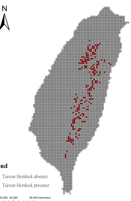
of Table 3, which is calculated by A/(A+C) , and X-axis is 1-specificity, which is calculated by B/(B+C). ... 30 Figure 4. Flowchart of methodology in this study ... 37 Figure 5. 212 occurrence and 3784 absence samples of Taiwan Hemlock from Third
Forest Resource and Land-Use Inventory (TFRLUI) ... 39 Figure 6. 408 occurrence of Taiwan Hemlock from National Vegetation Diversity
Inventory and Mapping Project (NVDIMP) ... 40 Figure 7. DCA odination of 6 sub groups of Taiwan Hemlock. ... 58 Figure 8. Cluster analysis dendrogram of 6 sub groups of Taiwan Hemlock. ... 61 Figure 9. PCA ordination of Taiwan Hemlock with 4 surveyed environtment variables
including ASP, CUR, ELE, PLA, PRCSP, PRCSR, PRCAU, PRCWT, PRCME, PRCSU, PRO, SLP, STH, SVF, WI, and WST. ... 65 Figure 10. PCA ordination of Taiwan Hemlock with 16 extracted environtment
variables including ASP, CUR, ELE, PLA, PRCSP, PRCSR, PRCAU, PRCWT, PRCME, PRCSU, PRO, SLP, STH, SVF, WI, and WST. ... 69 Figure 11.Normal Q-Q plot of 8 extracted environmental variables ... 76 Figure 12. Histogram of 8 extracted environemtal variable between absence and
presence localities. Y axis represents the relative frequency of counts of sample.
... 78 Figure 13. PCA ordination of Taiwan Hemlock and 8 extracted environtment variables
including CUR, PRCSU, PRCWT, SLP, STH, SVF, ELE and WST…………...80 Figure 14. Tree plot of classification and regression tree (CART) analysis with 6
groups of 196 Taiwan Hemlock presence localities and 16 extracted
environmental variables from RIAL. ... 84
vii
Figure 15. Prune tree of CART analysis from Figure 13 shows how each split affects the deviance. ... 85 Figure 16. Missclassification of tree plot from Figure 13 shows how each split reduces
misclassification number. ... 85 Figure 17. Tree plot of classification and regression tree (CART) analysis with 5
groups (combining V1 and V6 into V1) of 196 Taiwan Hemlock presence localities 16 extracted environmental variables from RIAL. ... 87 Figure 18. Tree plot of CTT analysis with 6 groups of 196 Taiwan Hemlock presence
localities 16 extracted environmental variables from RIAL. ... 89 Figure 19. Differences on AUC among 7 environmental variable combinations,ALL,
CA, CART, CIT, PC1, PC2, PC3, and 5 type of occurrence localies, V1, V2, V3, V5, and Vall at 3 different kinds of map resulotion ... 93 Figure 20. Probability pictures of Maxent model which uses environmental variable
combination by CART method. ... 96 Figure 21. 11 Responese Curves of environmental variables for Maxent prediction of
All occurrences data Vall vegetation type. X-axis is the range of environmental variable value and Y-axis is the logistic output of probability of presence (40 × 40 m in resolution). ... 102 Figure 22. Null model test for Vall data set. The black dot on the bottom-right is the
AUC value generated by the predictied model Maxent. ... 106 Figure 23. Potential vegetation map of Taiwan Hemlock with threshold equals to
MaxKappa and 4 sub-units of Taiwan Hemlock vegetation types (V1, V2, V3, and V5). ... 110
viii
Table of Tables
Table 1. Predicted vegetation modeling (PVM) techniques with continuous and
categorical data ... 14
Table 2. Some application of SDMs in ecology fields ... 18
Table 3. 2 × 2 classification table (confusion matrix) ... 25
Table 4. Indices derived from confusion matrix of Table 3 ... 26
Table 5. Elevation range of Taiwan Hemlock from National Vegetation Diversity Inventory and Mapping Project (NVDIMP) and Third Forest Resource and Land-Use Inventory (TFRLUI) data sets ... 41
Table 6. List of environmental variables ... 42
Table 7. Data format of SDM ... 48
Table 8. Pearson and Kendall correlation between surveyed environmental gradients and DCA and PCA axes. (N= 196) ... 62
Table 9. Pearson and Kendall correlation between 16 extracted environmental gradients and DCA and PCA axes. (N= 196) ... 62
Table 10. Variance extracted first 10 axes of PCA from 4 surveyed environmental variables. ... 64
Table 11. Variance extracted first 10 components of PCA from 16 extracted environmental variables. ... 68
Table 12. Correlation analysis for extracted environmental variable of 196 localities of Taiwan Hemlock. ... 74
Table 13. Basic and descriptive statistic of presence localities (N = 196) ... 75
Table 14. Basic and descriptive statistic of absence localities (N = 3770) ... 75
Table 15. t-test of absence and presence localities ... 77
Table 16. Percentage of variance and cumulative percentage of variance from extracted 8 components of PCA. ... 82
Table 17. First 6 eigenvectors each scaled to its standard deviation of PCA. ... 83
Table 18. Summary of CART analysis with 6 groups of 196 Taiwan Hemlock Presence localities 16 extracted environmental variables from RIAL. ... 88
Table 19. Summary of CIT analysis with 6 groups of 196 Taiwan Hemlock Presence localities 16 extracted environmental variables from RIAL. ... 90
ix
Table 20. Summary of all approaches selecting influential environmental variables to distribution of Taiwan Hemlock. Character “V” means the variable is selected by the method. ... 91 Table 21. Results of the multiple Behrens-Fisher tests for 4 vegetation types, V1, V2, V3,
V5, and Vall Taiwan Hemlock localities Vall by 2-sided p-value. ... 95 Table 22. Contributions of the environmental variables to the Maxent model with Vall,
V1, V2 and V3 ... 103 Table 23. The 8 methods of threshold selection produced by PresenceAbsence package of R ... 104 Table 24. Threshold dependent indices for each occurrence unit in threshold = 0.5 .. 105 Table 25. Threshold dependent indices for each occurrence unit in threshold =
MaxKappa ... 105 Table 26. Confusion matrix of potential natural vegetation map of Taiwan Hemlock by
Vall with threshold equals to MaxKappa. ... 108 Table 27. Confusion matrix of potential natural vegetation map of Taiwan Hemlock by
V1 with threshold equals to MaxKappa. ... 108 Table 28. Confusion matrix of potential natural vegetation map of Taiwan Hemlock by
V2 with threshold equals to MaxKappa. ... 108 Table 29. Confusion matrix of potential natural vegetation map of Taiwan Hemlock by
V3 with threshold equals to MaxKappa. ... 108 Table 30. Confusion matrix of potential natural vegetation map of Taiwan Hemlock by
V5 with threshold equals to MaxKappa. ... 109 Table 31. Indices derived from confusion matrix of potential natural vegetation map of
Taiwan Hemlock with threshold equals to MaxKappa. ... 109
1
Chapter 1: Introduction
1.1 Background
The question about plants and animals’ current distribution is discussed for a long history and makes many ecologists find the explanation. Many modelers root in species-environment relationships to establish many modeling approaches for solving this question (Guisan and Thuiller, 2005). Analysis of the species’ geographic distribution has always been an important issue in vegetation science, and is currently focused by other sub-disciplines such as biogeography and landscape ecology. The relationship between environmental gradients and vegetation distribution is one of the most important issues examined in vegetation science (Miller et al., 2007). The ability to quantify the relationship leads to predict potential distribution of vegetation and is applicable for predicting spatial distribution under changing environmental conditions, such as climate change occurring (Miller et al., 2007).
The purpose of potential vegetation field survey is to understand plant ecology and apply to ecological conservation, landscape restoration, and landscape planting (Yang, 1997). Survey data for estimating or predicting potential vegetation according to plant ecology, or plant geography, explain forest composition, structure, and function, further more, the relationship with environmental variables and its succession stage. Those data information allow us to predict the next succession, current or future distribution of species and vegetation and are useful for forest ecosystem management, biological conservation, and landscape restoration. On the contrary to traditional survey analysis,
2
Chiou et al. (2006) introduced GIS technique and several models are rapidly developed in recent years. Combining vegetation mapping and analysis of satellite images with GIS generate predictive vegetation model, a new approach for analysis species/vegetation and environmental variables (such as Gu et al., 2006; Tsao, 2007;
Yen, 2007) (Franklin, 1995; Guisan and Zimmermann, 2000; Scott et al., 2002) and this study is also based on the new approach.
Climate change has become an important focused issue in recent years, as a basis for assessing whether anthropogenic greenhouse effect has enhanced climate change and how the continuingly growing greenhouse gas concentration will lead to an unknown future climate. According to the IPCC’s Third Assessment Reports (TAR, IPCC, 2001), the average temperature of global surface has increased by about 0.6 °C in the past century, and to the IPCC’s Forth Assessment Report (AR4), warming in the last 100 years has increased by 0.74 °C in global average temperature. This is above the 0.6
°C increase in the 20th century prior to the Third Assessment Report (IPCC, 2007).
Taiwan has been moving toward a warmer and drier climate. Enhanced precipitation is observed in the limited areas in the limited times, however, a systematic trend (or change) is not observed (Hsu, 2002). In general, under constant climate change and global warming conditions possibly forces the distribution area of current vegetation diminishing, and increases the risk of species extinction. To predict the change of distribution of species under different climate scenarios is essential to assess the risk of species extinction under climate change (Thomas et al., 2004). Thus, the first mission is to establish predictable models for species potential distribution range (Tsao, 2007).
3
Previous ecologist in Taiwan mainly focused on classifying the plant communities and identifying the relationships between plant societies and environmental variables (i.e. Su, 1984a; 1984b). Island of Taiwan has a great diversity of fauna and flora due to a high degree of topographical complexity and an about 4000 m variation in altitude (elevation). A large proportion of Taiwan is not easy to access for field survey due to its hilly topography. Available field data might not be completely enough to support decision making of conservational or environmental policies (Song et al., 2007).
Species distribution models provide a possible way to fill up the gap of incomplete vegetation data (Franklin, 1998).
Projections of species distribution under climate and environmental change are of great scientific and social relevance, and basing on species distribution models (SDMs) make some assumptions such as species not adopt to global dispersal in evolution and consistency of limiting factors (Dormann, 2007). Although some of the assumptions are ecologically untenable, the predictions of the SDMs are still a useful reference to policy maker for climate change impact assessment and conservation management. This study examines the relationships between distributions of dominant species, Taiwan Hemlock (Tsuga chinensis (Franch.) Pritz. ex Diels var. formosana (Hayata) Li and Keng) of alpine forest in Taiwan, and climatic and topographical environmental variables. Not only traditional statistical approaches, but importance of new direction of data mining approaches in analyzing relationships between species and environmental factors will lead more precise insight and performance on SDMs prediction.
4
1.2 Objective
Although SDM are widely spread in many fields, the analysis of relationship in species-environment is still methodologically not well organized. This study will focus on comparing statistical and data mining methods to find the suitable environmental layers for building the spatial distribution of Taiwan Hemlock vegetation. Additionally, some studies of SDM application can be found in Taiwan (Gu et al., 2006; Tsao, 2007;
Yen, 2007) but fewer studies in Taiwan considers the comparison of difference model setting (like Song, 2007). Smaller grid size of the predicted background can reflect the more detail of topographical variables than climatic variables but is time consuming due to a very large data size for model estimation. Contrarily, larger grid size of background is much faster when calculating but lacks of or reduces detail information of the meso-environmental variables. Thus, this study also takes grid size, predicted area, locality units, and environmental selection of the model input into account.
Pervious studies for SDMs (mentioned later in Ch. 2 literature review) were using multiple model combination to improve the predictive accuracy for each species’ spatial distribution, however, combining different hierarchy units of species and vegetation to increase the predictive accuracy are seldom seen in resent researches. Therefore, comparing model techniques combination and species-vegetation unit combination is to compare and combine different SDMs to synthesize potential vegetation map of Taiwan Hemlock another goal of this study. The combination criteria are utilized to determine the binomial potential distribution area that Taiwan Hemlock may occur. There are 4 main objectives listed as follow:
5
1. Using data mining approach (classification and regression tree, CART and conditional inference tree, CIT) compared to statistical approaches (detrened correspondence analysis, DCA, principal component analysis, PCA and correlation analysis, CA) for analysis of relationship between species distributions and environmental variables.
2. Assess how localities inputs of different vegetation and species based sub-units on distribution modeling relate to environmental variables.
3. Evaluate how difference grid resolution affects the model performance and relationship between target species and environmental variables.
4. Model combination and synthesis of potential nature vegetation maps.
6
Chapter 2: Literature review
2.1 Climatic Factor and Vegetation Distribution in Taiwan
Alpine ecosystem’s unique characteristic environment, such as strongly wind blowing, shallow soil, low temperature, snow cover, is unsuitable for growing and is sensitive to climate change (Luckman, 1990; Walther, 2004). Therefore, monitoring alpine ecosystem for climate change impact assessment on alpine forest is a very important approach worldwide (Luckman, 1990).
Vegetation Zone differentiation in Taiwan changes along with altitude gradient and variation of vegetation in Taiwan is specified by vegetation zones or vegetation biomes divided by different elevation (Liu, 1962; Su, 1984b; Su, 1992). Su (1984a; 1984b) described the relationships between vegetation zones and climate factors and tried to divide the range of vegetation distribution by temperature factor. Su (1984b) investigated vegetation of Chou-Shui river basin in mid-Taiwan and established the relationships between elevation and temperature by regression analysis and determined the up and low limits of elevation for every vegetation zone. Su’s vegetation zone (1984b) is a high hierarchy classification unit and each zone may contain different forest types due to differentiation of topography, soil, or succession stage.
Many ecologists considered latitude and elevation are the main factor to species distribution (Kellman, 1980; Su, 1985; Su, 1987; Guissan et al., 1998, Liang, 2004; Yen
et al., 2007). Previous studies on vegetation science in Taiwan restricted to financial
7
support and thus most vegetation survey sites limited within local area like boundary of watershed, naturally conserved area, or administrative area, such as Su’s (1988) study site in Single-seed Juniper conserved area, Su (1984b) in Chou-shui river basin, Liu et
al. (1999) in Sha Li Shian watershed, and Fu (2002) in Dan-Da area. Those local studies
with varied purposes, methods, and location, which boundary doesn’t represent the real boundary of species’ distribution, hardly integrate the vegetation distribution in Taiwan (Chiou et al., 2006).Chiou et al. (2006) analyzed the distribution characteristic of Taiwan Hemlock community in Taiwan using cluster analysis and compared with environmental conditions, altitude, latitude, and warmth index. Two methods of the comparison are order and inter-specific association. Yen et al. (2007) and Tsao (2007) firstly introduced the model techniques for modeling species distribution over the whole Taiwan Island.
Yen et al. (2007) used second-order logistic regression in generalized linear model (GLM) to estimate the probabilistic distribution of Taiwan Hemlock in Taiwan by two of the most important environmental variables, latitude and altitude. Tsao (2007) used generalized additive model (GAM) to establish the relationships between distribution ranges and environmental variables for six conifer species, Chamaecyparis obtusa var.
formosana, Chamaecyparis formosensis, Abies kawakamii, Tsuga chinensis, Picea morrisonicola, and Pinus taiwanensis, of Taiwan. Tsao’s result shows all of the six
GAM models select the variable of mean annual temperature for building model, in other words, distribution of six plant species is affected by mean annual temperature.Annual precipitation, however, is not selected by any of the six models. Therefore, the probable explanation may be Taiwan Island receives abundant precipitation all year
8
round, so precipitation is not a limiting factor for vegetation distribution in Taiwan (Kuo, 1978; Yen, 2007).
2.2 Data Mining Approach in Environmental Factor Analysis
2.2.1 CART
Classification and regression tree (CART) is a kind of decision tree. Breiman et
al.’s (1984) CART is a common basis for some ensemble procedures such as bagging
(Breiman, 1996), random forest (Breiman, 2001), and stochastic gradient boosting (Friedman, 2001a). Kriegler (2007) mentioned four key aspects of CART are (i) Splitting criteria for regression tree, (ii) Pruning and knowing when to stop making splits, (iii) Costs and the relation to priors, and (iv) Obtaining fitted values. CART can handle both numeric (regression tree) and categorical (classification tree) predictor and response variable.De’Ath and Fabricius (2000) described CART is ideally suitable for analyzing the complex ecological data, which is usually strongly non-linear, involving higher order iteration, unbalanced, and containing missing values. Because CART is flexible and robust analytical methods and can handle for such complex data. Furthermore, CART results are simple to understand and easily interpretable by its graphical representation with root (undivided data) at the top and branches and leaves (final groups) underneath.
The explanation for variation of a single response variable for trees is using one or more explanatory variables (continuous/categorical) to repeatedly split the data into more
9
homogeneous groups, which is defined by a single rule based on single explanatory variable, but to remain the tree reasonably small. Splitting is continued until an overlarge tree is grown and then pruning reshapes it back to the desired size. Each group/leaf is characterized by a typical value of the response variable (mean value for numeric response and distribution for categorical response), the number of observations in the group, and the values of the explanatory variables that define it. The tree is represented graphically, and this aids exploration and understanding.
Trees are interactive exploration and both descriptive and predictive for patterns and processes. De’Ath and Fabricius (2000) stated advantages of CART including: (i) the flexibility to handle different types of response variables, numeric, categorical, ratings, and survival data; (ii) invariance to monotonic transformations of the explanatory variables; (iii) the capacity for interactive exploration, description, and prediction; (iv) ease and robustness of construction; (v) ease of interpretation by graphical representation; and (vi) the ability to handle missing values in both response and explanatory variables. Therefore, CART is an alternative to many traditional statistical techniques, such as multiple regression, analysis of variance, logistic regression, log-linear models, linear discriminant analysis, and survival models for complement or representation (De’Ath and Fabricius, 2000).
2.2.2 CIT
CIT is an abbreviation of conditional inference tree, which can deal with recursive partitioning for continuous, censored, ordered, nominal and multivariate response variables and the implementation utilizes a unified framework for conditional inference
10
developed by Strasser and Weber (1999). Hothorn et al. (2006) described conditional inference framework for recursive binary partitioning can be solve two fundamental problems of exhaustive search procedures, (i) over fitting and (ii) a selection bias towards covariates with many possible splits or missing values, by (i) pruning procedures and (ii) embedding tree-structured regression models into a well defined theory of conditional inference procedures, based on invariant p-value.
Roughly, the algorithm of CIT works as follow steps: (i) Test the global null hypothesis of independence between any of the explanatory and the response variables and stop if this hypothesis cannot be rejected (i.e. the explanatory and response variables in a specific splitting node are not independent to each other). Otherwise select the explanatory variable with strongest association to the response variable with measuring a p-value corresponding to a test for the partial null hypothesis of a single explanatory variable and the response variable. (ii) Split binaurally in the selected explanatory variable. (iii) Recursively repeat steps (i) and (ii).
The stop criterion in step (i) is either based on multiplicity adjusted or univariate p-values and it is shown that the predictive performance of the resulting trees is as good as the performance of established exhaustive search procedures (Hothorn et al., 2006).
This statistical test ensures that the right side of the tree is grown and no form of pruning or cross-validation. The selection of the explanatory variable to split in is based on the univariate p-values preventing a variable selection bias from explanatory variables with too many possible splitting points. Moreover, the prediction accuracy of trees with early stopping is equivalent to the prediction accuracy of pruned trees with unbiased variable selection.
11
2.3 Ecological Niche and Species Distribution Model
2.3.1 Predicted Vegetation Modeling
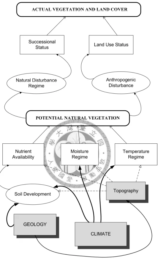
Maps of vegetation composition have traditionally been produced by field survey and photo interpretation, but these methods are costly and inefficient. Predictive vegetation modeling (PVM) can be defined as predicting the distribution of vegetation across a landscape based on the relationship between the spatial distribution of vegetation and relevant environmental variables (Franklin, 1995). Fraklin (1995) provided the relationship between environmental variables and their process affecting distribution of potential natural and actual vegetation (Figure 1).
12
Figure 1. Conceptual model showing relationships and processes between climatic determinants, direct gradients, potential natural vegetation and actual vegetation (revised from Franklin, 1995)
13
PNV is determined by environmental determinants (climatic, geographic, and topographic factors) which changes local soil nutrients, moisture, and temperature.
After natural and/or anthropogenic disturbance, like competition, succession, land-use, actual vegetation and land-use type form as mosaics on landscape.
To evaluate potential vegetation, predicting vegetation mapping (PVM) is firstly considered. Three steps described by Franklin (1995) and Chen (1997) for PVM are (i) Traditional approach: explanation by aerial photos or numeric vegetation map from geographic mapping combines with geographic information system (GIS) for decision making. (ii) Numeric approach: establishment of mathematical relationship between environmental variables (such as temperature, precipitation, soil type) and traditional field survey records helps to understand the distribution of vegetation. (iii) Predicting vegetation mapping. Step 1 actually not real analyze the data as step 2 does, in the other words, the spatial pattern of species is not only simply digitizing the survey data, but also establishes the statistically or mechanistically mathematical relationship with environmental variables.
Development methodology of PVM traced to Kessell’s (1976) series studies on connecting real spatial object with abstract spatial model by gradient modeling with GIS in Glacier National Park, USA; Box (1981) used empirical model to generate distribution of global vegetation with global plant communities and macro-scaled climatic variables. After this point plenty of relevant studies followed. Table 1 integrates the methods of recent 20 years studies for PVM.
14
Climate-Vegetation classification model, one of PVM, assumes that major vegetation of any site is the result of environmental factors and considers climatic variables playing an important role on it (Tuhkanen, 1980). Köppen (1931) and Holdridge (1967) established the classification of global vegetation and its life zone, Walter (2002) divided 9 zonal biomes in macro-scale mapping of vegetation, Chiu et al.
(2005) mapped Holdridge’s life zones at Taiwan. Ecologists also consider the dominant vegetation type is response by reaction of climatic variables and every climatic zone should have its vegetation type (Whittaker, 1975).
Table 1. Predicted vegetation modeling (PVM) techniques with continuous and categorical data (revised from Franklin, 1995; Chen, 1997)
Dependent variable
Independent variable
Continuous Mixed Categorical
Continuous
RM ANCOVA ANCOVA
RT MANCOVA MANCOVA
GLM RT RT
GLM) GLM
Categorical
MLC MLC with priors Contingency Table
Logit (GLM) Logit (GLM) Logit (GLM)
DA GAM GAM
GAM CART CART
CART NN NN
GA GA ES ES
Notes: ANCOVA: Analysis of Co-Variance; CART: Classification and Regression Tree; DA:
Discriminant analysis; ES: Expert System; GA: Genetic Algorithms; GAM: Generalized Additive Models;
GLM: Generalized Linear Models; MANCOVA: Multivariate Analysis of Co-Variance; MLC: Maximum Likehood Classification; NN: Neural Network; RM: Regression Tree; RT: Regression Tree.
Chen (1997) described two scales for studying PVM. (i) Regional scale and (ii) Local scale. Study range of regional scale is considering global and continental area and
15
the environmental variable is mainly climatic variable. In this scale the climate-vegetation model belongs to static model (Lowell, 1991) and is based on assumption of the equilibrium between distribution of vegetation and environmental variables. (Leniha and Neilson, 1993),and this assumption is acceptable for larger area and loner time (Cramer and Leemans, 1993). Study range of local scale is smaller than regional scale such as a watershed and the environmental variables are selected for this scale such like topographic variable, slope, aspect, and soil type. In this scale, predicting of PVM is not only the static model, but also considers the topographic and micro-climate variables to project the active procedures of species’ birth, growth, and death (Urban et al., 1991). However, the complex background knowledge about climate-vegetation interaction is needed for the dynamic models (Brovkin, 2002).
Unfortunately, few dynamic mechanisms of interaction of vegetation and ecosystem are well developed (Foley et al., 1998).
Chen (1997) introduced three stage of model building in GIS: (i) establish spatial database, digitalizing the survey records and environmental variables for spatial analysis and further application in GIS. (ii) Set up the mathematical relationship between species and environmental variables. (iii) Combine the mathematical model and GIS tool and database to output and display the results.
Potential natural vegetation maps are applied to communicate the natural baseline conditions for assessing ecosystem health, predictions of vegetation distribution which is caused by responding to environmental factors to management, and determination of potential resource value (Jansen et al., 2002). Danijela (2003) applied predictive vegetation model to manage and conserve the developed area based on the PNV
16
conception. PNV concept is not only for vegetation mapping, but also for land-use development and as a potential and basic reference for describing and integrating ecosystems (Hardtle, 1995; Seibert and Conrad-Brauner, 1995). For example, PNV represents the climax stage of vegetation under the stable environmental condition and can be used as a guide for ecosystem restoration (Danijela, 2003). In Japan, many cities have their own actual and potential vegetation maps for land-use planning and integrate the PNV studies concluding which native species is better for planting on the area.
(Miyawaki et al., 1987; Miyawaki and Fujiwara, 1988; Miyawaki, 1988). PNV is also applied in simulating global and local climate change impacts, such as Cha (1998) estimated potential change of forest area under 2 times CO2 concentration.
2.3.2 SDM/ENM
Species distribution models (SDMs) or ecological niche-based models (ENMs) are two kinds of the PVM techniques and are empirical models relating field survey observations to environmental predictor variables, which is based on statistically or theoretically derived response layers (Guisan and Zimmermann, 2000). SDMs describes the spatial distribution of a species or species groups, as a function of environmental predictor variable such as latitude, longitude, altitude, climate, topography, land-use type, vegetation type, soil conditions, and so on. Species presence-only and presence-absence data are two major formats of the SDMs’ explanatory variables and the former data type is usually easier to obtain by historical records such as museum specimens, private collections, or field surveys. In other words, the potential species distribution model (PSDM) is developed from a set of environmental variables for a set of rasters, together with a set of data localities where the species are observed and
17
predicts the suitability for the target species as functions of environmental variables.
(Phillips et al., 2006; Prates-Clark et al., 2008).
Guisan and Thuiller (2005) describe three phases of SDMs by author’s personal communication to S. Ferrier:
(i) Non-spatial statistical quantification of species–environment relationship based on empirical data,
(ii) expert-based (non-statistical, non-empirical) spatial modeling of species distribution.
(iii) Spatially explicit statistical and empirical modeling of species distribution.
Species distribution models (SDMs) of plants and animals are interested widely in the last two decades and applied many issues in ecology, biogeography, evolution and, in conservation biology and climate change research(Guisan and Thuiller, 2005), such as predicting species distributions from museum and herbarium records (Elith and Leathwick, 2007), predicting future range of species distributions under climate change impacts (Thomas et al., 2004), mapping species ranges and species richness (Graham and Hijmans, 2006), predicting the invasive spread of a cactus species in Australia (Johnson, 1989) (quoted in Pearson and Dawson, 2003), assessing the climatic determinants of the distribution of several European species (Hengeveld, 1990) (quoted in Pearson and Dawson, 2003), enhancing a regional vegetation map (Franklin, 2002), biodiversity conservation (Rodríguez et al., 2007) …etc. Table 2 shows the application of SDMs in ecology fields.
18
Table 2. Some application of SDMs in ecology fields (revised from Guisan and Thuiller, 2005)
Type of use References
Quantifying the ecological niche of species
Austin et al. (1990), Peterson et al.
(2002), Vetaas (2002), Sattler et al.
(2007), Rissler and Apodaca (2007), Raxworthy et al. (2008) Testing biogeographical, ecological and
evolutionary hypotheses
Leathwick (1998), Anderson et al.
(2002), Graham et al. (2004b)
Assessing species invasion and proliferation
Beerling et al. (1995), Peterson (2003), Sanchez-Flores (2007), Wang et al. (2007)
Assessing the impact of climate, land use and other environmental impacts on species distributions
Thomas et al. (2004), Thuiller (2004), Early et al. (2007), Dormann (2007)
Suggesting unsurveyed sites of high potential of occurrence for rare, endemic, threatened species
Elith and Burgman (2002),
Raxworthy et al. (2003), Engler et
al. (2004), Zimmermann et al.
(2007) Supporting appropriate management plans for
species recovery and mapping suitable sites for species reintroduction
Pearce and Lindenmayer (1998)
Supporting conservation planning and reserve selection
Ferrier (2002), Arau´jo et al.
(2004), Pape and Gaubert (2007
Modeling species assemblages (biodiversity, composition)/vegetation from individual species predictions
Guisan and Theurillat (2000), Cairns (2001), Ferrier et al. (2002), Graham and Hijmans (2006), Rodrguez (2007), Saatchi et al.
(2008)
Predicting distribution of high value trees Prates-Clark et al. (2008)
Vegetation mapping support
Scott et al. (2001), Franklin (2002), Cawsey et al. (2002), Tatsuhara and Antatsu (2007)
19
ENM is slightly difference in the definition to SDM. Models of ecological niches are designed to estimate the potential niche’s area of the target species, and thus ENM predicts broader range than actual distribution (Phillips et al., 2006; Peterson et al., 2008).
James and McCulloch (1990) stated all parametric statistical models face to the problem with highly non-Gaussian distribution data such as most environmental variables. Stocktwell (2006) described:
“The ideal ENM method will (1) be capable of modeling a wide range of responses, (2) allow critical examination of assumptions, (3) be a simple approach that will not fit inappropriate functions, but (4) will handle extremely non-linear data, and (5) will efficiently turn an increasing flood of data from satellites, geographic information systems and climate model outputs into simple, scalable ENMs.”
2.3.3 SDMs and Ecological Theory
Niche based models like some of SDM or ENM (Maxent, GARP, GAM …etc) representing the approximation of species’ ecological niche in the examined environmental layers (Phillips et al., 2006). ENM is based on the idea of ecological niches defined as the set of conditions under which a species is able to maintain populations without immigration (Grinnell, 1917; 1924; Hutchinson, 1957; Hutchinson, 1978; and Austin et al., 1990). The ecological niche includes the fundamental niche, which consists of a set of conditions for species’ long-term survival, and realized niche, which is subset of fundamental niche for species’ actual occupation (Hutchinson, 1957).
20
Therefore the realized niche of a species may be smaller than its fundamental niche due to disturbances from human influence, biotic interaction (such as competition), geographic barriers, and/or natural disasters, and such factors are influential to its survival range and prevent the species from fully spreading its ecologically potential niche (Pulliam, 2000; Anderson and Mart´ınez-Meyer, 2004; Phillips et al., 2006). Thus niche based models estimate the approximation of species’ realized niche in environmental layers considered, however, the departure between realized and fundamental niche remains unknown in practice (Phillips et al., 2006). Realized niche can be estimated by removing areas that species is known or inferred not to inhabit from the predictive distribution such as areas suitable for the target species without colonized due to geographic barriers (Peterson et al., 1999; Anderson, 2003), biotic interactions (Anderson et al., 2002), and human influences (Anderson and Mart´ınez-Meyer, 2004).
Phillips et al. (2006) described the ecological assumption of environmental variables used for modeling are (i) temporal correspondence, (ii) scale, (iii) space and time. Temporal correspondence will be existed when using locality record that investigated very long time age for current land-cover classification (Anderson and Mart´ınez-Meyer, 2004). Mackey and Lindenmayer (2001) defined environmental variables for different scale: (i) global and meso-scales: climatic variables such as temperature and precipitation, (ii) meso- and topo-scales: topographic variables such as elevation and aspect, and (iii) micro-scales: land-cover variables such as forest canopy.
Su (1983) also introduced the classification of factors affecting species habitat: (i) direct/indirect factors, (ii) scales, (iii) affection, and (iv) sources. For source classification environmental variables influence habitat divided into 4 categories:
21
(i) Climatic factors: such as radiation, air temperature, precipitation, wetness.
(ii) Edaphic factors: also called soil factors, such as soil type, soil temperature.
(iii) Physiographic factors: also called topographic factors, such as aspect, altitude, slope, curvature.
(iv) Biotic factors: such as anthropogenic or biotic interactions or disturbances.
SDM has applied in Taiwan vegetation science for just a few years. Song et al.
(2007) compared the model performance of three SDM techniques, Maxent, GARP, and GAM, by evaluating sensitivity, specificity, and area under receiver operating characteristic (ROC) curve. Tsao (2007) used GAM to establish the relationships between distribution ranges and environmental variables for six conifer species,
Chamaecyparis obtusa var. formosana, Chamaecyparis formosensis, Abies kawakamii, Tsuga chinensis, Picea morrisonicola, and Pinus taiwanensis, of Taiwan.
2.3.4 MAXENT
Maxent program for maximum entropy based machine-learning modeling technique predicts species geographical distributions and is firstly introduced by Phillips et al. (2005). Maxent model’s estimation is based on a decision theoretic perspective as robust Bayes estimation (Phillips and Dudı´k, 2008) and simulates predictions from data with incomplete information to estimate a probability distribution by finding the probability distribution of maximum entropy (Della Pietra et al., 1997) (i.e. the Maxent approach assumes that the occurrence data of incomplete empirical probability distribution can be approximated with a probability distribution of maximum entropy subject to environmental layer’s constraints, and use this
22
approximated distribution for predicting a species potential geographic distribution (Phillips et al., 2005). Phillips and Dudı´k (2008) described the Maxent model uses the species’ occurrence data to define the region of probability with maximum entropy. The probability distribution π over the set X of plots is non-negative value and the sum of π(x) is one, where the x is the sample of the population X. The π is displayed in terms of
“gain”—the log (the number of rasters) - the log (loss) (i.e. the average of the negative log (probabilities of the sample locations) (Prates-Clark et al., 2008) and coincides with the potential distribution stated by biologists (Phillips et al., 2004). The simple function of environmental variables are a set of real-valued variables and called features, and the constraints are the mean of predictive features required to be near the empirical average over the occurrence sites (Phillips et al., 2006).
Initially, each environmental variable is treated as potentially an important predictor variable to develop the model. Jackknife test re-sampling method (Peterson and Cohoon, 1999) of Maxent’s internal procedures reduces the bias of correlated environmental variables and to diagnose which environmental variables were the most important variables for building models. The environmental variables with the highest gain means higher the relative importance of variables that potentially, contribute to generating the SDM (Phillips et al., 2004).
Maxent displays the influence of each environmental variable in response curve diagrams. As the Maxent model is an exponential model (Della Pietra et al., 1997), the probability of prediction is proportional to the exponential contribution of each environmental variable (Phillips et al., 2006). The response curves in version 3.2.1 are in logistic (probability) space, rather than exponent (linear) space, so they're easier to
23
interpret. Statistical approaches for evaluating model performance such as dependent omission rate and independent AUC of ROC analysis are also including the internal procedures of the Maxent. Some other features of Maxent 3.2.1 can visit Maxent website (http://www.cs.princeton.edu/~schapire/maxent/) for more information. Maxent with pros and cons were reviewed by some study. The advantages of Maxent include the usage of both categorical and continuous environmental data (Prates-Clark et al., 2008).
2.4 Model Performance Evaluation
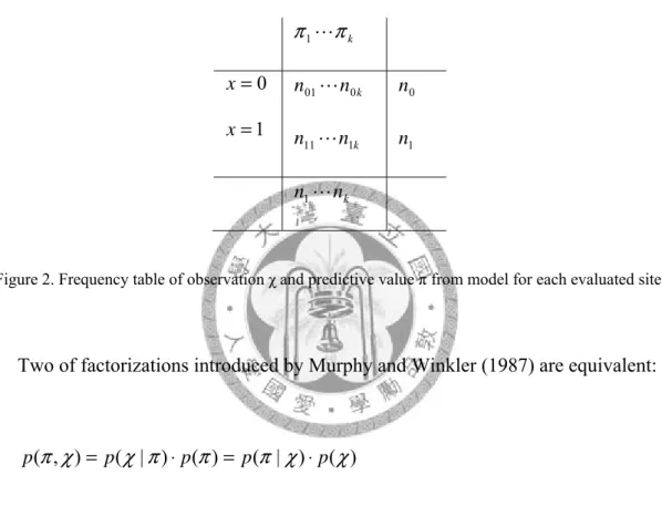
Model performance can be evaluated by the accuracy of model predictions, the interpretability and rationality of the explanatory variables, and the validity of predicted shape of response curves (Pearce and Ferrier, 2000). A good prediction includes both reliable and discriminatory prediction. Reliable prediction means the accurate estimation of probability for a species’ occurrence site and discriminatory prediction means the ability to discriminate the species occupied or unoccupied site in the study area. The model predicts each site from the study area with a probability π for species occurrence and the observation from each site consists of presence or absence of the target species χ. Murphy and Winkler (1987; 1992) factorized the joint distribution of π and χ into a conditional distribution (
p
(χ
|π
) orp
(π
|χ
))and a marginal distribution (p
(π
) orp
(χ
)) as shown in Figure 2, wherep
(χ
|π
) andp
(π
) reflect model calibration and refinement respectively;p
(π
|χ
) andp
(χ
) represent the ability to discriminate and base rate (prevalence) respectively. If the model is well calibrated then the points should lie along a 45° line of the scatter plot for predicted probabilities24
comparing with observed occurrence and if the is well discriminated then little overlap between presence/absence distributions on the plot of frequency distribution of the predicted values for occupied sites comparing with unoccupied sites. The prevalence needs to be moderately large for examining the predictive performance of a model (Pearce and Ferrier, 2000).
π
kπ
1L=0 x
=1 x
n
kn
01L 0n
kn
11L 1n
0n1
n
kn
1LFigure 2. Frequency table of observation χ and predictive value π from model for each evaluated site.
Two of factorizations introduced by Murphy and Winkler (1987) are equivalent:
) ( )
| ( ) ( )
| ( ) ,
(
π χ p χ π p π p π χ p χ
p
= ⋅ = ⋅Therefore since the base rate (prevalence) is a constant, a model which has good calibration and refinement must also have a good discrimination, on the contrary, however, a good discrimination is not necessarily with good calibration and refinement.
These two aspects of model performance, calibration/refinement and discrimination/base rate reflect the reliable prediction of absolute value about how closely the predicted probabilities match the occurrence proportions and the ability of prediction to discriminate the observed presence to absence of predictions.
25
2.4.1 Confusion Matrix for Measuring Discrimination Performance
2 × 2 classification table (Table 3) often examines the model performance by comparing predicted value and actual observation (Pearce and Ferrier, 2000).
Generally thinking, greater numbers of both observed/predicted presence and absence (A and D in table 3) imply a good performance of the prediction, on the other hand, greater numbers of predicted presence and absence but actually absence and presence (B and C in Table 3) tell a bad performance of the prediction. False positive (B) and false negative (C) are also called omission (including unsuitable sites in the prediction) and commission (leaving out from distributional area) respectively (Peterson et al., 2008).
Predicted presence or absence is determined by predicted probability value which is higher or lower than the specific threshold. The four condition of the classification table can calculate four more indices: sensitivity, specificity, false positive fraction, false negative fraction, and other measures of model performance listed in Table 4.
Table 3. 2 × 2 classification table (confusion matrix), each of the values A to D represents the number of species observed (revised from Pearce and Ferrier, 2000;
Wang et al., 2007)
Observed
Presence Absence
Predicted
Presence A B A+B
Absence C D C+D
A+C B+D A+B+C+D
Note: A: true positive, B: false positive, C: false negative, D: true negative
26
Table 4. Indices derived from confusion matrix of Table 3 (revised from Fielding and Bell, 1997, Pearce and Ferrier, 2000;Wang et al., 2007; Tsao, 2007)
Index Description and Formula
Sensitivity
Number of positive sites correctly predicted
=
A Total number of positive sites A+C
Specificity Number of negative sites correctly predicted
= D
Total number of negative sites B+D
False Positive Fraction
Number of false positive predictions
=
C Total number of positive sites A+C
False Negative Fraction
Number of false negative predictions
=
B Total number of negative sites B+D Accuracy
(Correct classification rate)
Number of total sites correctly predicted
=
A+D Total number of sample sites A+B+C+D
Misclassification rate
Number of total misclassified sites
=
B+C Total number of sample sites A+B+C+D
Overall diagnostic power Total number of negative sites
= B+D
Total number of sample sites A+B+C+D
Prevalence
Total number of positive sites
=
A+C Total number of sample sites A+B+C+D
Positive predict power (PPP)
Number of positive sites correctly predicted
=
A Total number of predicted positive sites A+B
Negative predict power (NPP)
Number of negative sites correctly predicted
=
D Total number of predicted negative sites C+D Note: A: true positive, B: false positive, C: false negative, D: true negative
27
Table 4. Indices derived from confusion matrix of Table 3 (revised from Fielding and Bell, 1997, Pearce and Ferrier, 2000; Wang et al., 2007; Tsao, 2007) (cont.)
Index Description and Formula
Odds-ratio
Ratio between total correctly predicted and total
errors =
AD CB
Kappa (A+D)-{[(A+C)(A+B)+(B+D)(C+D)]/(A+B+C+D)}
(A+B+C+D)-{[(A+C)(A+B)+(B+D)(C+D)]/(A+B+C+D)}
Normalized mutual information (NMI)
-Aln(A)-Bln(B)-Cln(C)-Dln(D)+(A+B)ln(A+B)+(C+D)ln(C+D) (A+B+C+D)ln(A+B+C+D)-((A+C)ln(A+C)+(B+D)ln(B+D)) True Skill Statistic (TTS) Sensitivity + Specificity – 1
Area Under ROC Curve (AUC) In ROC curve, 1- specificity values are plotted on X axis and sensitivity values are plotted on Y axis respectively.
Note: A: true positive, B: false positive, C: false negative, D: true negative
The sensitivity represents true positive rates. A greater true positive rate indicates model has higher ability to predict species presence when observed presence occurs. On the contrary, the value of specificity represents the true negative rate which indicates model ability to predict spices absence when observed absence occurs. Landis and Koch (1977) have suggested 3 ranges of agreement for Kappa statistic K: (i) poor; K < 0.4, (ii) good; 0.4 < K <0.75, (iii) excellent; K > 0.75.
2.4.2 Threshold Independence AUC
The abbreviation of AUC means area under ROC curve. ROC means receiver operating characteristic analysis which is firstly introduced in evaluation the ability to receive radar signals and applied to medical field (Wang, 2007) and the broad application in many ENM and SDM studies (take Elith et al., 2006, Guisan et al., 2007
28
for instance) happened in resent ten years. Figure 3 is an example demonstrated the ROC curve an AUC value. ROC analysis plots “sensitivity” (equal to 1 - omission error rate) against “1 minus specificity” (equal to commission error rate) (Cantor et al., 1999) and calculates the area under ROC curve (AUC), and then compare the predicted AUC against null expectation (the area under the line from origin to the upright corner of the graph) probabilistically (Peterson et al., 2008). Figure 3 is an example of ROC analysis.
Y-axis is sensitivity of Table 3, which is calculated by A/(A+C), and X-axis is 1-specificity, which is calculated by B/(B+C). The procedure of ROC analysis is using threshold to generate points on ROC plots. For a continuous probability distribution, larger threshold means smaller distribution area than smaller threshold does, thus a specific threshold selection leads to a proportion of presence/absence’s distribution area.
The specific threshold selection implies selecting different threshold for dividing the continuous probability distribution into binomial presence/absence parts and leads to changing the values of the evaluated indices in Table 3 such as sensitivity, specificity, and accuracy. The feature of ROC analysis is threshold independent and from prevalence and often used for evaluating accuracy of diagnostic tests (Swets, 1988;
Tsao, 2007). To achieve this independency, ROC analysis estimates all thresholds of the probability distribution (from 0 to 1) to plot each value of sensitivity against 1 – specificity generated by specific threshold on the scatter plot of ROC and joints each points to become the ROC curve and the area under this curve is AUC. The ROC analysis represents the tradeoffs between the omission and commission error and AUC represents a specific metric for evaluating diagnostic procedures because it is a representation of the average sensitivity over all possible specificities (Prates-Clark et
al., 2008). If a larger threshold is selected then the area of predicted presence contains
partial observed presence points and area of predicted absence contains almost observed29
absence points, and therefore, the ROC algorithm almost doesn’t falsely identifies absence, but fails to indentify most presence and generates a point with larger omission and smaller commission plotted near down-left corner (0, 0) of the plot. Continuously diminishing the threshold to a smaller one, the area of predicted presence contains almost observed presence points and area of predicted absence contains fewer observed absence, and thus, the algorithm indentifies most true presence correctly, but misclassifies most absence as positive and generates a point with smaller omission and larger commission plotted near the up-right comer (1, 1) of the plot. Ideally the top-left corner (0, 1) of ROC plot means the algorithm correctly indentifies every true presence and never misclassifies a true absence as a presence (Peterson et al., 2008).
30
Figure 3. ROC analysis by PresenceAbsence package in R. where Y-axis is sensitivity of Table 3, which is calculated by A/(A+C) , and X-axis is 1-specificity, which is calculated by B/(B+C).
Prates-Clark et al. (2008) described 2 data sets for evaluating predicted models: (i) a training data set for model building, and (ii) a test data set for model validation. A low omission rate (high sensitivity) of species presence is essential for predicting predicted range of distribution (Anderson et al., 2003). After selecting a threshold, model performance can be evaluated using both: (i) the extrinsic omission rate (using test dataset); (ii) the proportional predicted area (Prates-Clark et al., 2008).
31
Unlike sensitivity and specificity, area under ROC curve (AUC) value is independent from prevalence and often used for evaluating accuracy of diagnostic tests (Swets, 1988; Tsao, 2007). AUC value combines sensitivity and specificity to estimate model performance and ranging from 0.5-1. According to Swets (1988), AUC value is 0.5, that means accuracy of model happen by chance; AUC value falling between 0.5-0.7 means the discrimination of model is low; AUC value falling between 0.7-0.9 means the prediction is responsible good and can be applied to other researches; AUC value is grater than 0.9 representing very good model accuracy.
2.5 Model Comparison and Combination
As motioned formerly, SDM has become an expanding tool in the areas of conservation biology, climate change research, land-use/land-cover change assessment, and biodiversity estimation (Guisan and Zimmermann, 2000). Although there are many available statistical methods, previous model comparison studies show that the prediction accuracy from different models was little in difference (Franklin, 1998;
Vayssières et al., 2000; Cairns, 2001; Thuiller et al., 2003; Muñoz and Felicísimo, 2004). Moisen and Frescino (2002) compared predictive performance of five methods, linear models (LM), generalized additive models (GAM), classification and regression trees (CART), multivariate adaptive regression splines (MARS), and artificial neural networks (ANN), however, still found little difference among those methods (Moisen and Frescino, 2002). And besides, Elith and Burgman (2003) found greater disparities in accuracy among the plant species being modeled than among the four modeling
32
methods that were compared. Guisan et al. (2007) compared 10 model techniques, BIOCLIM, BRUTO, BRT, DOMAIN, GDMSS GAM, GLM, MAXENT, MARS, and OM-GARP, 30 tree species in Switzerland, and found the greater difference in model accuracy among species than model techniques and also found that location error and sample size reduced predictive performance of many models, whereas resolution of environmental grids had little effect on most model techniques, and no model technique is able to rescue difficultly predictive target species. Therefore, to maximize accuracy of multiple model performances is needed since there is no study founding a best model (Gilmer, 2007).
Model combination (also known as consensus modeling, composite models, forecast aggregation, forecast synthesis and forecast combination) is one of the alternative ways to improve predictive accuracy of multiple models (Gilmer, 2007).
Clemen (1989), Reid (1968), Bates and Granger (1969), and Batchelor and Dua (1995) suggested model combination is optimal and can yield greatest benefits for predictive accuracy. In niche model predictions, multiple models can be created for each species and the model outputs combined to determine locations present or absent of each species (Anderson et al., 2002a; Lim et al., 2002; Anderson et al., 2003; Araújo et al.
2006). Olmeda and Fernández (1997) combined models by a simple voting scheme, called “majority-vote criterion”, to determine the presence/absence of locations and founded that less accurate models combination produced less predictive accuracy than the single models. Araújo et al. (2005) also suggested model averaging gave best predictive performance and accuracy. Clemen (1989) concluded model combination as:
33
“Combining forecasts has been shown to be practical, economical and useful.
Underlying theory has been developed, and many empirical tests have demonstrated the value of composite forecasting. We no longer need to justify this methodology. We do need to find ways to make the implementation of the technique easy and efficient.”
Gilmer (2007) used three kinds of model combination approaches: (i) Composite (Anderson et al., 2002a; and Lim et al., 2002), (ii) Averaging (See and Abrahart, 2001), (iii) Summation (Anderson et al., 2003). Composite (i.e. majority vote criteria) uses conditional statement to determine the final prediction. For instance, if there three binary outputs from individual models, any location are given value 2 representing presence, otherwise absence. Averaging means averaging standardized probabilistic outputs from different individual models and determined presence/absence by threshold.
Summation gives useful visual explanation by summing the binary outputs from individual models (i.e. the higher number the location gets, the more model supports).