光線追蹤法之平行化加速結構於多核處理器

(1)

國立臺灣大學電資學院電機工程研究所碩士論文

Department of Graduate Institute of Electrical Engineering College of Electrical Engineering and Computer Science

National Taiwan University Master thesis

光線追蹤法之平行化加速結構於多核處理器

Parallel KD Tree Acceleration Structures for Ray Tracing on Multi-Core Processor

曾至正

Chih-Cheng Tseng

指導教授：鄭士康博士 Advisor: Shyh-Kang Jeng, Ph.D.

中華民國 98 年 6 月

June, 2009

(2)

(3)

致謝

對3D 動畫技術很嚮往的我，這幾年來每天總要寫程式，也自己念了不少數學。

不斷改進遊戲動畫引擎，幾年下來，寫了超過十萬行 C++，也足以自豪。同學們

都知道，晚上十點後還有一個人在實驗室寫程式。

這樣的我，卻考進了電機所，為了畢業，曾經嘗試接觸一些電路、電子、晶片設計的領域，最後還是放棄了。搞了老半天，後來鄭士康老師拉了我一把。回首這段路程，更加清楚自己要的是什麼，幸好，我仍在一條熱血的道路上前進。

我能夠完成這篇論文，最要感謝的是鄭士康老師。鄭老師對學生沒有什麼要求，如果有的話，就是把自己的研究做好。鄭老師處處為學生著想，卻從來不問學生能幫他什麼，身為一個資深教授，卻對每個學生都是一視同仁，言出必信，

每個學生都很感謝他。在510 這段期間，可說是魚與熊掌兼得，不但完成了論文，

而且做了許多有意義的事。

印象深刻的是三位開授平行計算的老師，曾于恒老師是流體力學的專家，有時我有數學上的問題，也去請教他；黃乾綱老師對各種程式很有一套，又非常熱心；

鄭振牟老師是第一位在台大開授 CUDA，讓人耳目一新。資工所圖學組的三位老

師，雖然沒有直接指導過我，但給也過一些不錯的建議。對其他指導過我的師長們，也要說聲謝謝。

感謝實驗室的宗恩、天麟學長，在無形中教了我許多事情。仲耀大、呂大、徐大、SOLO 大、世霖大等同學，都是幽默風趣的強者，再佐以俊嘉、亞聖等搞笑風格，實在覺得這裡不像是實驗室。

也要特別提到動畫工作坊的小鐵、小茶、怡萱、伊寧等，大家一起熬夜做動畫，

在我論文交出去的當天，剛好是我們的發表日，太神了！

(4)

(5)

Abstract

Global illumination is vital in nowadays computer animation, where ray tracing is

used to simulate the lighting in real world. Due to the massive computation requirement,

the algorithm cannot be applied in real time interactive application. In the era of post

Moore’s law, desktop CPU has more and more cores, 8-core and 16-core CPU are going

to appear, one can see the prospect of ray traced games.

KD tree is able to fast cull out the empty spaces in the scene, while other structures

lack this feature. Especially for unstructured scenes with fast changing geometry where

local updates of the structure degrade immediately and a fast reconstruction is preferred.

In the thesis we will skip other parts of ray tracing, but focus on the parallel

implementation of the KD tree on multi-core CPU, that is the key to speed up. At

beginning we decompose the scene space into sub regions. These sub regions are going

to be processed by different cores of CPU. Finally we merge the subtrees into one. We

achieve a near fully parallel construction and still preserve a high quality tree.

Keywords: KD tree, global illumination, ray tracing, animation, interactive, game

(6)

摘要

全域照明是現今 3D 電腦動畫所必備，其原理在於應用光線追蹤法模擬真實光

線，但其計算量極大，故遲遲未能應用在即時性的互動遊戲。在後摩爾定律的年

代，桌上處理器核心數量不斷提高，八核及十六核CPU 不久後將釋出，可以預見

全域照明法即將出現在電腦遊戲當中。

在各種加速結構中， KD tree 能夠最有效率的分割場景。特別在沒有關聯性組織的場景中，快速移動的物體，局部性的結構更新很快就失去效力，在這種狀況下通常需要全域性的快速結構重建。

本論文將略過ray tracing 其他部分，而專注於 KD tree 多核平行化的深入探討，

這是加速ray tracing 的關鍵。將場景分割成許多子空間，再使用多核心 CPU 分別

處理分割過的子空間，最後再將子樹合併。我們得到了一個接近完全平行化的建造方法，同時仍然維持著樹的高品質。

關鍵字：全域照明、光線追蹤、電腦動畫、互動、遊戲、空間分割、二元樹

(7)

LISTS OF FIGURES

Fig. 2-1 Whitted style recursive ray tracing ... 4

Fig. 3-1 Split at (A) spatial median (B) object median (C) minimum SAH cost ... 8

Fig. 3-2 Events of triangle ... 9

Fig. 3-3 Incremental sweeping for split ... 10

Fig. 3-4 Conventional binning and min-max binning on one axis ... 15

Fig. 4-1 At the time the sweeping reaches the plane p, we have NL = 2 and NR = 2 ... 18

Fig. 4-2 Augmented min-max events of the AABB ... 19

Fig. 4-3 A trivial and general method for event classification ... 19

Fig. 4-4 DFS KD tree construction (Blue for internal, green for leaf, red for empty), IDs in brackets are undefined ... 22

Fig. 4-5 BFS KD tree construction (Blue for internal, green for leaf, red for empty) ... 24

Fig. 4-6 BFS construction with node pool implemented as array of structure (AOS) ... 25

Fig. 5-1 Domain partitioning in serial ... 28

Fig. 5-2 Merging of sub-arrays ... 29

Fig. 5-3 Parallel 1D binning for domain partitioning ... 31

Fig. 5-4 Parallel 3D binning for domain partitioning ... 32

Fig. 6-1 KD-Restart ... 34

Fig. 8-1 A bitonic merge sort of 2048 elements on CUDA, with block size = 512 ... 47

Fig. 8-2 Unsegmented scan: reduction (left) and down-sweep (right) ... 48

(11)

Fig. 9-1 (a) Arm, 816 triangles (b) Kila, 4,110 triangles (c) Dragon, 65,533 triangles (d) Temple, 222,900 triangles ... 52

(12)

LIST OF TABLES

Table 9-1 Construction time (sec) with subtree construction in parallel .... 52 Table 9-2 Construction time (sec) with parallel subtree construction and parallel 1D binning ... 53 Table 9-3 Construction time (sec) with parallel subtree construction and parallel 3D binning ... 54 Table 9-4 Render time (4 threads) (sec) with subtree construction in

parallel ... 54 Table 9-5 Render time (4 threads) (sec) with parallel subtree construction and parallel 1D binning ... 55 Table 9-6 Render time (4 threads) (sec) with parallel subtree construction and parallel 3D binning ... 55

(13)

Chapter 1 Introduction

1.1 Outline of the Thesis

In the thesis we are going to thoroughly discuss various algorithms of the KD tree.

The thesis begins with the fundamentals of ray tracing in Chapter 2. In Chapter 3, the

state-of-the-art of KD tree construction is covered. We then present some optimizing

techniques in Chapter 4, also the pros and cons of DFS and BFS construction, SOA and

AOS node implementation.

Chapter 5 is about how the KD tree construction is mapped to multi-core processor.

Highly parallel implementations (the parallel domain partitioning with binning plus the

concurrent subtree construction) is addressed. The comparison of 1D binning and 3D

binning reveals the trade-off between the construction and traversal of the KD tree.

In Chapter 6 we show that the conventional KD-restart and KD-backtrack can be

easily powered with openMP.

The two fundamental operations on GPU are introduced in Chapter 7. The bitonic

merge sort and the segmented prefix sum can be used to accelerate the KD tree

construction. We also showed the implementations of the two algorithms on CUDA.

(14)

1.2 Contributions

For fast KD tree construction, some researchers use three events: starting, ending

and lying to classify the triangles. We have proposed a new concept called augmented

AABB, where only two events are needed. And we have proved that the augmented

AABB is more general, robust and efficient.

We have presented a comparison between the DFS construction and the BFS

construction with preallocated memory. And we found that construction with BFS

fashion outperform the conventional DFS construction. As far as we know, this

comparison is never done before.

For parallel domain partitioning, a prior work resorted to the 1D binning; we have

implemented and tested the 3D binning. Although the 1D binning performs faster, for a

partition more than 8 the 3D binning makes a good trade-off between the construction

time and the traversal time. This observation has never been proposed before.

(15)

Chapter 2 Background

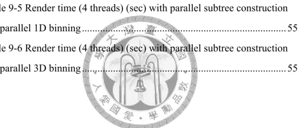
2.1 Ray Tracing

Phong’s model has dominated the screen of 3D games, where the light source is

assumed to be infinitely away from all the objects, and the radiance is merely from the

dot product of the surface normal and the light direction.

In physics, photons bounce from surfaces to surfaces, generate reflections and

refractions from different materials. If there are obstacles between an object and the

light source, the occluded object becomes shadowed, and that is what we want in 3D

games. The need for realism stimulates the research of ray tracing.

[33] proposed a simple but powerful model, sometimes called recursive ray tracing.

Rays are first shot from virtual camera through each pixel into the scene, they are called

“primary rays”, and their mission is to find the closest intersection point. And if there is

a hit point, a “shadow ray” is launched toward the light source to see if the light is

blocked or not. The ray incidence with the geometry surface determines the intensity of

radiance, combined with the property of material then we can calculate the shading.

Secondary rays are needed to generate the phenomena like reflection or refraction, and

(16)

these rays can be spawned recursively, contribute to the shading.

Fig. 2-1 Whitted style recursive ray tracing

2.2 Acceleration Structures

While millions of rays are looking for their nearest collisions in a scene with

millions of triangles, it is unlikely to apply a brutal search, instead we resort to some

advanced structures. The intersection test of a ray and a triangle is very expensive, and

for each ray we cannot afford too many tests, the ability to fast cull away most of the

triangles is the most important.

Structures like uniform grid, BVH (bounding volume hierarchy), BSP tree, OBB

tree (oriented bounding box), K-Dop, octree, KD tree, have been used in ray tracing.

(17)

Chapter 3 Related Work

3.1 Fast KD tree Construction

3.1.1 Introduction

KD tree is a variant of BSP tree, it is widely used in the area of computer graphics

and science computing, the relevant applications are not limited to ray tracing, but any

problem related to nearest neighbor search. For the scene with few triangles, the

construction time can be insignificant compared to the render time. However, modern

animations with elaborate scenes and detailed characters usually may have millions of

triangles, and the construction time becomes critical.

For earlier GPUs uniform grid was used [21, 22], the structure is simple but fits

badly to sparse scenes.

Although structures like BVH can efficiently represent some structured models like

characters, where a motion can be handled with local updates of BVH [9], unstructured

models like dynamics system make BVH degrade immediately, and a reconstruction

from scratch is necessary.

KD tree has been recognized as the best structure for ray tracing [11]. It is able to

(18)

fast cull away the empty spaces in the scene, which is crucial for wide open scenes

where the triangle distribution is sparse. And further, KD tree uses AABB (axis aligned

bounding box) as a proxy for geometry primitives, these axis aligned voxels offer

extremely fast traversal. Structure like OBB tree [8] is able to fit the primitives well,

however the arbitrary orientation make it much slow for traversal.

Variants of KD tree like B-KD tree [29, 34] and SKD tree [12] use two slabs for the

split, and simplify the problem of straddling triangles [14]. For such trees left node and

right node have overlapped region, and also the two empty spaces at the two ends can

be culled. However, they lack an optimized traversal approach like [4, 24, 25]. These

trees are not the mainstream and will not be discussed here.

3.1.2 Fast KD tree construction overview

KD tree construction begins as a global voxel which contains the whole scene,

called root node, then a top-down fashion binary split is proceeded recursively. Each

node is going to split into two children. The pattern continues until the current node no

longer has to split, by the time the leaf node usually has only a few triangles.

The process of fast KD tree construction in O(NlogN) can be roughly divided in

several stages :

(1) Termination criterion checking

(19)

(2) Determine the split axis

(3) Split position evaluation

(4) Classification of triangles

(5) Classification of events

(6) Splice to left and right node

Given a node, we first check some criteria to qualify the node for upcoming stages.

If the depth has reached a threshold, or the number of triangles within the node has

fallen below a user-specified value, the node then is tagged leaf. Otherwise the node is

an internal node.

To split a non leaf node, first we have to choose the split axis. Evaluation of

geometry distribution is not trivial and time consuming, the common sense is to always

choose the axis with longest extent, or choose in round robin fashion.

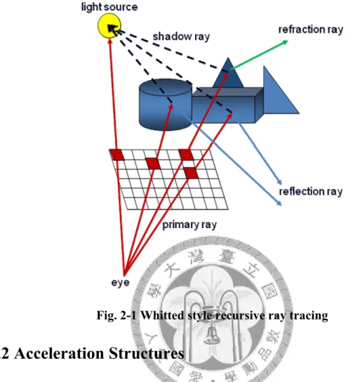
3.1.3 Surface Area Heuristic

Split at spatial median is easy, but inefficient. It is important to discard most of the

spaces and triangles as early as possible. Our goal is to terminate the ray as fast as we

can, and a carefully picked split can make a big difference. The trick is to produce large

chunks of empty space close to the root of the tree. [28] has mentioned “Benefits of a

good tree are not small”, and may be “several times faster than a mediocre tree”.

(20)

Fig. 3-1 Split at (A) spatial median (B) object median (C) minimum SAH cost

A cost model based on geometric probability of ray has been proposed [11, 15].

The model assumes the rays are uniformly distributed, and the likelihood a ray will

intersect the node is roughly proportional to its surface area. Also if the cost of

intersection is Ci, the cost of intersection test against N triangles roughly equals NCi.

Based on [15], the cost of tree can be expressed as follows.

T I tri

C :cost of traversal

C : cost of intersection test

N : number of triangles in the node

( ) ( )

( ) ^T ( ) ^t

All nodes All leaves

SA node SA leaf

C C

SA root SA root

=

∑

+

∑

^{N C}^ri ^I ^(3.1)

With this cost function, the same triangle may appear in different leaves, and will

be tested several times against the same ray. A correct version is derived as follows.

(21)

( ) ( )

( | |

( ) ( )

T I L R

SA left subnode SA right subnode

C C C C C

SA node SA node

= + + | |) (3.2)

Although theoretically CL and CR are going to be recursively evaluated, in fact this

approximation works great. The concept is called surface area heuristic, and based on

this we can pick the split to minimize the cost of the node.

3.1.4 Split Candidate

Theoretically on the split axis there can be infinite split candidates, nevertheless

the cost is piecewise linear along the axis, and it changes only at the AABB planes of

the triangle. What we have to consider are these plane positions, also called events of

triangle.

Fig. 3-2 Events of triangle [32] suggested that there are three kinds of event.

(22)

starting min position of triangle on the axis ending max position of triangle on the axis

lying min=max if the triangle is perpendicular to the axis

⇒

(3.3)

All events are sorted once at root in ascending order, the order is maintained during

the entire construction process. Every node has its own sorted event list, and to each

event we perform SAH evaluation. One thing to note is that if we do not maintain the

events as sorted, but merely compute the SAH cost for each event individually, then

each time we have to count again the triangles to the left and to the right, the complexity

is terribly O(N^2).

Taking the advantage of the sorted events, the number of triangles to the left and to

the right can be counted incrementally [19, 32]. At the first event, all triangles lie on the

right side, so NL is zero and NR has all. By sweeping over the events from left to right,

each time we simply increment the NL and decrement the NR, and the cost of all

candidates can be known in O(N). Record the event with the minimum cost as the split.

Fig. 3-3 Incremental sweeping for split

(23)

| +

i - i

| i

i

0 | 0 0

0 0

|

-1 - |

-1

p : Triangles starting on plane i p : Triangles ending on plane i p : Triangles lying on plane i

cost ( , , )

0 -

( 0; ; ){

- -

i L R

P L R

Pi i

i i

R R i i

i i

L L

SAH p N N

N p N N N p

for i i numEvents i

N p

N N p p

N N p

=

= = =

= < + +

=

= + ^|

}

i⁺+pi

(3.4)

A bonus for culling away empty space is suggested [25, 32]. The cost is scaled by

about 80% if we choose to split at the position where one side is empty.

Exact SAH evaluation can be approximated by coarsely sampling at finite discrete

positions [14]. Especially for nodes near the root this method saves a lot of time without

losing much accuracy.

Binning [14, 19, 27] is an alternative to incremental sweeping, the method also has a

sort-free like feature, and is able to fast evaluate the cost regardless of the number of

triangles. The main problem about binning is the accuracy of the SAH cost, and deeper

the node is, more obvious the problem has become. The issues about binning will be

discussed later.

3.1.5 Triangle Classification and Clipping

Once the split position has been decided, we are going to distribute the events to left

(24)

and right. However, some of the events belong to straddling triangles, which contribute

its events to both sides, and should be further clipped into two pieces.

So before we process the events directly, we want to tag these triangles as “LEFT”,

“RIGHT”, or “BOTH”. An efficient sweeping can be applied as follows.

(3.5)

Most of the triangles will be marked “LEFT” or “RIGHT”, and a few will remain as

“BOTH”, these triangles straddle the split plane, and need special care.

3.1.6 Event Classification and Generation

There is no problem about dealing with events associated with triangles marked

“LEFT” or “RIGHT”, these events will be copied to one side with the ascending order

unchanged. But for a straddling triangle, its “starting” event lies in left and its “ending”

event lies in right. And the triangle should be clipped into two polygons, one for each

side.

The precise way is to apply a Sutherland Hodgeman clipping to the triangle, two

polygons are generated. We have to calculate the AABB for the two polygons, and

replace the old events of the triangle with the new events of the two polygons, on both

axis

flag pos tri

for all t

side[t]=BOTH;

for all e && e ==splitAxis

if(e == ending && e <= splitPosition)side[e ]=LEFT;

else if(e == starting && e >= splitPosition)side[e ]=RIGHT;

(25)

sides. These new events should be merged with the event arrays to maintain the

ascending order.

The process of triangle clipping, with generation of new events and merging of

events can be an impact to performance. Fortunately in reasonable cases the number of

straddling triangles is minor.

A trivial way is to just copy these events to both sides, and update the events if they

exceed the boundaries.

3.1.7 Splice to two children

New memory is dynamically allocated for the two children, or the bias address is

incremented if we have preallocated pools.

3.1.8 Termination Criteria

The stages above are performed for each node split, and the ascending order of new

event lists are always preserved. The pattern continues until some of the criteria have

been achieved.

(1) The number of triangles of the node is smaller than a threshold.

(2) The depth of the node exceeds a threshold.

(3) The split position cannot be found for the node.

(26)

The first is mandatory, and the second can be optional. It is notable that we cannot

always find a split for every node. In a case where many triangles have the same

minimum and maximum on the split axis, the only two split candidates are the

minimum and maximum of the node’s AABB. The split like this will not be performed,

and we either switch to another split axis, or force the node to be a leaf.

3.1.9 Conclusion

All stages required for a node split are presented here.

(1) Termination criteria checking O(1) (2) Split axis picking => O(1)

(3) Incremental sweeping for split => O(N) (4) Triangle classification => O(N)

(5) Event classification, generation, and merging => O(N)

=>

(3.6)

Sum up all the stages we get O(N) for one node split. From an easy math the

complexity of the whole tree is derived as following.

(3.7)

This is the fastest we can get for KD tree construction so far. However, for

interactive games with millions of triangles even the best optimized algorithm is not

enough, and we have to look for help from hardware.

3.2 Parallel KD tree Construction on Multi-Core CPU

( ) 2 ( / 2) ... O(NlogN) T N = N+ T N = =>

(27)

3.2.1 Introduction

[27, 32] have demonstrated KD tree construction on multi-core CPU. They have

proposed the method to partition the scene domain into sub-regions, and build sub-trees

in parallel. [32] has done the domain partitioning in serial, and the scalability is

sub-linear with the number of processors. [27] has proposed a fully parallel

implementation with initial clustering based on binning, and achieved good scalability.

3.2.2 Binning

[19, 27] advocate the sort-free sweeping, but improve the performance by applying

coarser sampling, also called binning. Binning is similar to pigeonhole and bucket

sorting, which is originally devised for points. For triangles, the conventional binning is

improper for SAH evaluation, and a min-max binning is used instead [27].

Fig. 3-4 Conventional binning and min-max binning on one axis

3.2.3 Initial Clustering

(28)

There are two ways to construct the tree. First, all threads work together to build the

whole tree, the problem is that everyone needs to access all the primitives, this demands

large cache of all the processors and usually causes race condition. A better way is to

evenly divide the tree into subtrees, and each subtree is handled by exactly one thread.

This makes sense since subtrees can be stored in the local memory of the processor in

charge. Therefore each processor has its own primitive pools to work on, and the

memory traffics are reduced.

[19] used only one thread to do the initial partitioning task, and [27] proposed an

initial clustering in parallel. They first uniformly distribute all primitives to all

processors, and all threads run the binning on their portion of primitives. And by

splitting at object median they evenly divide the bins of the selected dimension into

segments, and then each segment of the bins is assigned to one thread. Now all the

threads know its own set of primitives, and subtrees are built in parallel.

(29)

Chapter 4 Optimizing KD tree Construction

4.1 Augmented AABB

We have made some modifications to the fast KD tree construction [32]. They

mentioned that three kinds of event are used: “starting”, “ending” and “lying”, triangles

lying in the split plane should be placed into either left or right, depends on SAH

evaluation [32]. However, from our experiments we observed that additional conditions

are needed for “lying” events, and these conditions complicated the process.

We do not see the benefits from using “lying” events; instead we advocate the

method using minimum and maximum of the AABBs [19]. This is also more general

and robust, since KD tree is not always for triangles; any primitive can be an element of

KD tree and can be easily fit into an AABB.

Based on our observation, benefits are induced if we use the min-max events of the

AABBs.

(1) Only one bit flag is required to tell from minimum or maximum.

(2) The number of events is automatically double the number of triangles, on all

three axes.

(3) Simplify the incremental sweeping.

(30)

(4) Simplify the SAH cost function; eliminate the situation that some triangles lie on

the split candidate.

(5) Simplify the classification of triangles and events.

(6) Simplify the condition branch in ray traversal.

Based upon our observation at least 10% speedup is achieved. Unfortunately some

problems arise from the modification. The incremental sweeping for SAH now becomes

as follows.

{

i

0 0

-1 -

-1

cost ( , , )

} 0

( 0; ; )

-

i L R

L R

i i

R R i

i i

L L i

SAH p N N

N N N

for i i numEvents i

N N p

N N p⁺

=

= =

= < + +

=

= +

(4.1)

Triangles lying on the plane orthogonal to the split axis generate minimum and

maximum of the same value. You can see that such triangles are omitted by SAH

function, since by the time the triangles have already been deleted from NR, but have

not been added to NL. Let us see the case below.

Fig. 4-1 At the time the sweeping reaches the plane p, we have NL = 2 and NR = 2

(31)

A remedy to this is to augment the AABB; we decrease the minimum and increase

the maximum by an epsilon. Now the SAH function works correctly.

Fig. 4-2 Augmented min-max events of the AABB

4.2 A Trivial and General Method for Event Classification

The standard event classification for straddling triangles [32] requires Sutherland

Hodgeman clipping and merging of the new events with the originals. The approach

seriously complicates the event classification, and cannot be applied when primitives

other than triangle are used. Here we use a general and robust method to handle the

straddling AABBs. The pseudo algorithm is as follows.

Fig. 4-3 A trivial and general method for event classification

(32)

for all e on the splitAxis S0 if(side[e] == LEFT)

Event_L[S0][numE_L[S0]++] = Event[S0][e];

if(side[e] == RIGHT)

Event_R[S0][numE_B[S0]/2 + numE_R[S0]++] = Event[S0][e];

if(side[e] == BOTH)

if(Event[S0][e] is ending)

Event_L[S0][numE_L[S0] + numTriBOTH + numE_BL[S0]++] = Event[S0][e];

Set the event position as splitPosition

Event_R[S0][numTriBOTH + numE_R[S0]++] = Event[S0][e];

if(Event[S0][e] is starting)

Event_L[S0][numE_L[S0]++] = Event[S0][e];

Event_R[S0][numE_BR[S0]++] = Event[S0][e];

Set the event position as splitPosition

for all e on the non-splitAxis S=(S0+1)%3 and S=(S0+2)%3 if(side[e] == LEFT)

Event_L[S][numE_L[S]++] = Event[S][e];

if(side[e] == RIGHT)

Event_R[S][numE_R[S]++] = Event[S][e];

if(side[e] == BOTH)

Event_L[S][numE_L[S]++] = Event[S][e];

Event_R[S][numE_R[S]++] = Event[S][e];

(4.2)

This method works excellently in the situation where most of the primitives have

similar sizes. And further, this method helps us handle non-triangle based surfaces.

4.3 Using Preallocated Pools

A major bottleneck of KD tree construction is the rapid memory allocation. [2, 27]

have proposed the concept of pre-allocated pool, and we have used a similar method.

(33)

The difficulties arise from the prediction of the final size of the pools. The method

to precisely estimate the size of nodes and leaves of the whole tree remains unknown.

[27] has used chunks of memory linked into lists for nodes and leaves. They perform

the construction in DFS fashion, and if the current chunk is full they allocate a new one.

Similarly we deploy one node pool and one leaf pool. At each level we first check if

the remaining space is enough for the next level. If necessary we allocate a larger pool

and move over the original arrays.

Based upon our experiments, the construction with preallocated pools is at least

twice faster than the one using dynamic allocation.

4.4 DFS KD Tree Construction with Preallocated Pools

KD tree is generally constructed in DFS. [27] proposed a DFS construction with

preallocated memory, here we present a similar implementation.

The node pool and leaf pool grow constantly during construction. Merely two

temporary arrays are needed, array A for left sub-nodes and array B for right sub-nodes.

As one node splits into two, we replace the events of the node with the events of its left

child in array A, and the events of its right child are “pushed” to array B. Array B

actually serves like a stack, each time the split reaches a leaf, the events of the newest

node in array B are “popped” to array A. Node split always takes place in array A.

(34)

Fig. 4-4 DFS KD tree construction (Blue for internal, green for leaf, red for empty), IDs in brackets are undefined

Note that while the nodes reside in the stack (array B), their node ID are still

undetermined. The node is assigned an ID and added to the node pool only after it is

(35)

popped to array A.

4.5 BFS KD Tree Construction with Preallocated Pools

We perform the construction in BFS style, each time we process one level of the tree.

The same two temporary arrays are needed. All the nodes of the first level reside in

array A. After we perform the split all the children are moved to array B. And next time

array A becomes the input. The two arrays are used alternately until the maximum level

is reached.

Any node generated is moved to the node pool, and its bias address in the pool will

be record as the left or right child of its parent node. Also any node detected as leaf will

have its events moved to the leaf pool.

(36)

Fig. 4-5 BFS KD tree construction (Blue for internal, green for leaf, red for empty)

4.6 KD Tree Construction: DFS VS BFS

The DFS fashion benefits from always choosing the left child to split, and there is

no need to store the AABB min/max. Therefore it consumes less memory than the BFS

fashion.

At traversal stage, DFS has another advantage of always placing the left child

immediately after the node in the node pool. This increases the data coherent and may

perform better when the cache size is small. The fashion is necessary for efficient

traversal [13, 20].

The BFS construction demands many fewer iterations, only one iteration for one

level. On the other hand, DFS suffers from rapid stack operations, each time a node is

split, the right child has to be pushed to array B; and each time the split reaches a leaf,

one node in array B has to be popped to array A. The frequent memory traffic

considerably limits the performance.

Based upon our experiments, construction using BFS is about 25% faster than that

using DFS. Thus we have adopted BFS as our default throughout all the upcoming

chapters.

(37)

4.7 KD Tree Node Structures: AOS VS SOA

Although storing nodes as array of structures (AOS) may be more straightforward,

structure of arrays (SOA) is necessary for parallel implementations. Especially for some

architecture like NVIDIA CUDA, where structure and class are not supported and SOA

must be used.

For traversal as KD-restart rather than KD-backtrack, the AABB min/max can be

omitted, as well as the pointer to parent.

Fig. 4-6 BFS construction with node pool implemented as array of structure (AOS)

(38)

(39)

Chapter 5 Parallel Construction on Multi-Core CPU

5.1 OpenMP Standard

Nowadays there are two major parallel programming models; one is openMP [6],

based on shared memory architecture, the other is MPI [23], or the message passing

interface. OpenMP has a huge advantage of keeping the sequential and parallel codes

identical. Directives are used to tell the compiler whether to parallel the region or not,

this preserves the original sequential codes. OpenMP is also portable; the codes can be

ported to various machines without modification. Here we choose openMP as our

parallel implementation.

5.2 Domain Partitioning in Serial

Our goal is to divide the scene into disjoint regions with roughly the same number

of primitives, and each region represents a subtree. Simply divide at primitive median

and we can have two sub-domains with roughly equal primitives.

At first one thread is in charge of the construction, the only difference is that we

simply use the event median rather than incremental sweeping SAH for the split

position. The construction is proceeded until a certain level, where each node of the

(40)

level will be the root of a subtree at the next stage. For example, if we need eight

subtrees, the construction is performed until level three is done.

The events of these nodes are moved to the event arrays of the subtrees.

Fig. 5-1 Domain partitioning in serial

5.3 Subtree Construction in Parallel

Let each subtree have its own node pool and event pool; we assign them to threads

and run the subtree construction in parallel.

#pragma omp parallel for

(int 0; ; )

( );

for sub sub numSubtree sub buildSubTree sub

= < + + (5.1)

According to the number “sub” it has been assigned, each thread knows which pools

to work on.

The subtree construction is totally the same as the regular construction we have

(41)

mentioned in the previous chapter.

5.4 Merging of Subtrees

After the subtree construction is done, every subtree has its own node pool and leaf

pool. As we would hope to maintain the same ray traversal codes, we must merge the

sub-arrays into a whole one.

Fig. 5-2 Merging of sub-arrays

5.5 Event Sorting on GPU

Since all events are sorted at root only once, and the ascending order is maintained

during the overall construction, much time can be saved if we can do the sorting in

(42)

parallel. For a model with 60k triangles, there are 120k events on all three axes, thus we

have to do a sorting of 120k elements 3 times. We use a bitonic merge sort on GPU for

the sorting; the details are discussed in Chapter 6.

Although GPUs afford extreme performance for the root event sorting, the domain

partition here is still performed in serial. Also it is unlikely to expect that every desktop

has a decent GPU card, let alone a laptop. The implementation differs from various

GPUs, and we know that NVIDIA is not the sole vendor in the market.

5.6 Domain Partitioning in Parallel Using 1D Binning

To achieve a higher scalability we must do the initial partitioning in parallel as well.

By intuition we would like to do the event classification in parallel, but this is not going

to work out. Multiple threads work together on the same event lists, this cause race

condition. Of course we can evenly distribute the events to threads, but in order to

maintain the ascending order additional merge sorts are inevitable.

Rather than partitioning the sorted events, we instead partition the triangles. We

pigeonhole all the triangles on one selected axis, this is called binning [27]. And by

accumulating the triangles one can decide at which bin the region is split. Finally we

will have regions with roughly equal number of triangles.

First we calculate the minimum and maximum of the whole scene on the three axes,

(43)

and find the axis with the longest extent to perform binning, this can be done in O(N). A

fixed number of bins are set on the selected axis. All triangles are evenly distributed to

threads, and all threads perform the min-max binning in parallel. And then we

increment one bin at a time to accumulate the triangles from the minimum to the

maximum, if the accumulated triangles are larger than the percentage (25% if 4 sub

regions), we mark the left boundary of the bin as one boundary of the sub region.

Fig. 5-3 Parallel 1D binning for domain partitioning

After all boundaries of the sub regions have been decided, we classify all triangles

into sub regions, also in parallel. Now all subtrees have roughly the same number of

triangles, and by sorting each subtree has its own sorted event list.

Not only are the triangles binned in parallel, but also the event sorting is done in

parallel. The scalability has improved drastically.

(44)

5.7 Domain Partitioning in Parallel Using 3D Binning

Binning on one dimension is easy, but may finally reach a “tipping point”. For a

partition of 8, 16 and up, the space becomes “slices of bread”. The quality of tree

degrades seriously, and we can see that the performance of ray traversal plunges.

A remedy to this is to perform the binning on all three dimensions. However,

another difficult arises as that we cannot bin all the triangles into its sub-region at one

step. Therefore the binning is factored into DFS or BFS fashion.

Fig. 5-4 Parallel 3D binning for domain partitioning

The 3D binning is slower, but better preserves the quality of tree. For a partition

fewer than 8 we still prefer 1D binning.

(45)

Chapter 6 Single Ray Traversal on Multi-Core CPU

6.1 The Standard Traversal

Given a constructed tree, every ray starts at the root, and goes down for a hit.

According to the split plane of the current node, the ray may intersect with only left or

right child, or both. If the ray intersects only with the left child, we can easily advance

the ray to the left child. A ray straddles the split slab must have intersections with both

children, by the direction sign on the split axis, either left or right will be traversed first,

and the other child will be pushed onto the stack. The pattern is repeated until the ray

has reached a leaf, and if the ray finds no hit in the leaf, one node will be popped from

the stack, where the down traversal starts again. This is the standard approach [18], on

the stack one node is closer to the ray origin than all nodes behind it.

6.2 The Stackless Traversal

The standard approach demands one stack per ray. Since for GPU the cores process

many rays simultaneously, and the shared memory among cores usually is limited, the

per ray stack approach becomes problematic. [7] presented two stackless traversal

methods, called KD-restart and KD-backtrack.

(46)

A segment of ray can be represented as a time interval [t_min, t_max]. At beginning

we have the entire range, and during the down traversal the interval [t_min, t_max]

keeps being modified until we reach a leaf. If there is no collision found in the leaf and

the ray has not reached its end, instead of popping a node from the stack we merely

advance the segment. At the time the new t_min is assigned the value of t_max, and the

traversal either restart from the root (KD-restart), or from the closest ancestor

(KD-backtrack).

Fig. 6-1 KD-Restart

Although theoretically KD-backtrack may be slightly faster than KD-restart, it

consumes much more memory space and may also cause additional burden on the

construction stage. The KD-backtrack requires additional information about a pointer to

(47)

parent and the parent node’s AABB (7 floats per node). Thus KD-restart has gradually

become recognized as a conventional traversal scheme [13]. Based upon our

experiments, KD-restart and KD-backtrack have indistinguishable performance. [7]

mentioned that the KD-restart is at most three times slower than the stack based

traversal.

6.3 Iterative Single Ray Traversal

For performance reason we implement the traversal as iterative “while loops” rather

than tail calls. Here we show our pseudo algorithm of KD-restart implemented as SOA.

(48)

(6.1)

(6.2) node = 0;

rayStop = false;

while ( rayStop == false ){

//Non-leaf node

if (KD_bLeaf[node] == false){

if (rayDir[axis] > 0) {

t_split = (KD_splitPoint[node] - rayStart[axis]) / rayDir[axis];

if(t_split >= t_max) node = KD_subL[node];

else if(t_split <= t_min) node = KD_subR[node];

else {node = KD_subL[node]; t_max = t_split;}

}

if (rayDir[axis] < 0) {

t_split = (KD_splitPoint[node] - rayStart[axis]) / rayDir[axis];

if(t_split >= t_max) node = KD_subR[node];

else if(t_split <= t_min) node = KD_subL[node];

else {node = KD_subR[node]; t_max = t_split;}

} else {

if(rayStart[axis] < KD_splitPoint[axis]) node = KD_subL[node];

else if(rayStart[axis] > KD_splitPoint[axis]) node = KD_subR[node];

else node = KD_subL[node];

} }

//leaf node else {

if(KD_bEmpty[node] == false) Hit = ray triangle intersection;

if(Hit) rayStop = true;

else {

if(t_max >= t_max_G) rayStop = true;

else {

t_min = t_max;

t_max = t_max_G;

//Restart node = 0;

} } } }

(49)

Note that the division by ray direction can be replaced with a precomputed

reciprocal.

6.4 Optimized Ray Triangle Intersection

The ray triangle intersection occupies a large fraction of the render time, [33]

mentioned that the fraction can be in a range of 75% to 95%.

[5] separated the ray traversal into two phases, the traversal control flow is handled

by CPU, and the ray triangle intersection tests are totally moved to GPU.

A conventional routine for the intersection test begins with a distance test, if the

distance between the ray origin and the triangle plane is in the interval, then there is a

chance to get a hit. The barycentric coordinates are computed to see if the hit point lies

inside the triangle [16, 17], note that we store the barycentric coordinates for the

afterward shading [30].

(1 )

( ) ( )

(0 , , 1)

P A B C A B C

P A B A C A

if the P is within the triangle

α β γ β γ β γ

β γ

α β γ

= + + = − − + +

− = − + −

≤ ≤

(6.3)

(50)

The project method [30] optimizes the barycentric calculation by projecting the

triangle and the hit point onto a 2D plane while preserving the barycentric coordinates.

The plane is chosen to have the largest projected area for numerical stability.

( ) ( )

* * * *

proj proj proj proj proj proj

P A B A C A

let b C A and c B A and p P A

p c b

bu pv bv pu cv pu cu pv bu cv bv cu and bu cv bv cu

β γ

− = − + −

= − = − = −

= +

− −

= =

− −

(6.4)

Note that the projected edges b = (bu, bv) and c = (cu, cv) can be precomputed. The

method is almost two times faster than the original [16].

In the same leaf we record the distance of the triangle that has been checked, and if

the next triangle has a farther distance it is discarded immediately. Only those with

shorter distance have to undergo the barycentric test.

6.5 Hashed Mailboxing

A ray may encounter multiple leaves which contain the same primitives. Mailboxing

is applied to record the triangles which have already been tested against the ray, this

avoids unnecessary tests. According to [2], a full sized table is impractical. We deploy a

similar hashed mailbox. For regular scenes with flat surfaces we did not see any

performance gain, but for those with bumps or folds there may be a benefit.

(51)

6.6 Parallel Single Ray Traversal on Multi-Core CPU

Since every ray is independent with others during traversal, we can simply distribute

the rays to threads and run in parallel. This is also called screen-space parallelization.

(52)

(53)

Chapter 7 SIMD Incoherent Ray Bundle Tracing

7.1 Data Level Parallelism with Streaming SIMD Extension

The Intel’s Streaming SIMD Extension (SSE) was first introduced on Intel’s

Pentium III, where additional eight 128-bit XMM registers were provided. Four 32-bit

floating point values can be packed in one XMM register, and via one instruction we

actually operate on four data sets. Versions after SSE2 also support four 32-bit integer

values.

The layout of data should be arranged in the structure of array (SOA) to be eligible

and beneficial for the SSE implementation.

Hand-written assembly codes are difficult to maintain, furthermore, it loses the

support of compiler’s rearrangement and optimization, which tightly relates to the

problem of data dependency and latency. The SSE intrinsic provides the performance of

assembly coding, and also preserves the optimizations from the compiler’s view.

7.2 Optimization with SSE Intrinsics

To eliminate the branches induced by if-else clause, a register level macro is applied

[2].

(54)

(7.1)

The reciprocal operation is costly, but is necessary for the inverse of ray direction. A

conventional way is to approximate it with a Newton-Raphson iteration [2].

(7.2)

Usually the _mm_movemask_ps is used to check the sign bits of the four ray results,

the branch will take place if at least one sign bit is asserted. As mentioned in [24], this

operation is expensive and can be replaced by _mm_movemask_epi8.

7.3 The Initial Clipping

Not every ray has a hit with the scene box; these rays are marked as invalid and will

not be performed during the traversal. At the very beginning, we have to clip each ray to

its valid interval.

inline __m128 BLEND4(const __m128 f, const __m128 a, const __m128 b){

return _mm_or_ps(_mm_and_ps(f, a), _mm_andnot_ps(f, b));

}

inline __m128 RECIPROCAL4(const __m128 a){

const __m128 rcp =_mm_rcp_ps(a);

return _mm_sub_ps(_mm_add_ps(rcp, rcp), _mm_mul_ps(_mm_mul_ps(rcp, rcp), a));

}

(55)

__m128 t_min4 = _mm_setzero_ps();

__m128 t_max4 = _mm_set_ps1(FLT_MAX);

//---t_min t_max clip on X---

__m128 tClip_min4 = _mm_mul_ps(_mm_sub_ps(_mm_set_ps1(m_min[0]), rayStart4[0]), rayDirR4[0]);

__m128 tClip_max4 = _mm_mul_ps(_mm_sub_ps(_mm_set_ps1(m_max[0]), rayStart4[0]), rayDirR4[0]) __m128 rayDirSign4 = _mm_cmpgt_ps(rayDir4[0], _mm_setzero_ps());

t_min4 = _mm_max_ps(t_min4, BLEND4(rayDirSign4, tClip_min4, tClip_max4));

t_max4 = _mm_min_ps(t_max4, BLEND4(rayDirSign4, tClip_max4, tClip_min4));

//---t_min t_max clip on Y---

tClip_min4 = _mm_mul_ps(_mm_sub_ps(_mm_set_ps1(m_min[1]), rayStart4[1]), rayDirR4[1]);

tClip_max4 = _mm_mul_ps(_mm_sub_ps(_mm_set_ps1(m_max[1]), rayStart4[1]), rayDirR4[1]);

rayDirSign4 = _mm_cmpgt_ps(rayDir4[1], _mm_setzero_ps());

//---t_min t_max clip on Z---

tClip_min4 = _mm_mul_ps(_mm_sub_ps(_mm_set_ps1(m_min[2]), rayStart4[2]), rayDirR4[2]);

tClip_max4 = _mm_mul_ps(_mm_sub_ps(_mm_set_ps1(m_max[2]), rayStart4[2]), rayDirR4[2]);

rayDirSign4 = _mm_cmpgt_ps(rayDir4[2], _mm_setzero_ps());

//---Clip the rayLength--- t_max4 = _mm_min_ps(t_max4, rayLength4);

//---Check the intersection--- bIntersection4 = _mm_cmple_ps(t_min4, t_max4);

(7.3)

7.4 SIMD Ray Triangle Intersection

There are two ways to do this [30]. First we can consider intersecting one ray with

four triangles. Obviously there is some problem with this; not every leaf has a multiple

of four triangles, and usually they have only one or two triangles. Also KD tree tends to

perform better with small leaves [31].

The alternative is to test four rays against one triangle. This makes sense because

(56)

rays in a bundle are from consecutive pixels, and usually have similar origins and

directions. There is much of a chance to have all four rays collided on one big triangle.

7.5 Omnidirectional Ray Traversal for KD Tree

The traditional SSE traversal requires that the ray bundle is coherent in direction,

that is, the four rays have the same signs in all three dimensions. Early exit is favored,

because the nodes traversed are in the ascending distance order from all four ray’s

origins. On the contrary, the need to classify the rays into coherent group and treat them

individually inevitably lowers the utilization of the SIMD fashion. An alternative way is

to cluster the rays into eight coherent groups, but it results in bad work sharing on

multi-core architecture.

Omnidirectional traversal [24] is devised to process incoherent ray bundles.

Compared with the coherent traversal, it greatly reduces the number of triangle

intersection tests and reports an average of 1.5X speedup [24]. However, it comes at the

expense of no early exit. We cannot ensure that either the left child or the right child is

traversed first for incoherent rays; the only thing we consider is whether both children

are traversed or not.

(57)

const __m128 mix0f = _mm_castsi128_ps(_mm_set1_epi32(0x0000ffff));

__m128 rayTracing4 = _mm_and_ps(_mm_castsi128_ps(_mm_set1_epi32(0xffffffff)), rayValid4);

while(_mm_movemask_ps(rayTracing4)){

if(kdg_bLeaf[node] == false){

DWORD axis = kdg_splitAxis[node];

__m128 timeHitSplit4 = _mm_mul_ps(

_mm_sub_ps(_mm_set_ps1(kdg_splitPoint[node]), rayStart4[axis]), rayDirR4[axis]);

__m128 maskDir4 = _mm_cmplt_ps(rayDir4[axis], _mm_setzero_ps());

__m128 maskNear4 = _mm_cmple_ps(t_min4, timeHitSplit4);

__m128 maskFar4 = _mm_cmpge_ps(t_max4, timeHitSplit4);

__m128 maskSelect4 = _mm_xor_ps(mix0f, maskDir4);

__m128 maskValid4 = _mm_cmple_ps(t_min4, t_max4);

__m128 maskHit4 = _mm_and_ps(maskValid4, BLEND4(maskSelect4, maskNear4, maskFar4));

int hit4 = _mm_movemask_epi8(_mm_castps_si128(maskHit4));

int hitRight4 = hit4 & 0xcccc;

int hitLeft4 = hit4 & 0x3333;

if(hitLeft4 == 0){node = kdg_subR[node];continue;}

if(hitRight4 == 0){node = kdg_subL[node];continue;}

PUSH(kdg_subR[node],

BLEND4(maskDir4, t_min4, _mm_max_ps(timeHitSplit4, t_min4)), BLEND4(maskDir4, _mm_min_ps(timeHitSplit4, t_max4), t_max4));

node = kdg_subL[node];

t_min4 = BLEND4(maskDir4, _mm_max_ps(timeHitSplit4, t_min4), t_min4);

t_max4 = BLEND4(maskDir4, t_max4, _mm_min_ps(timeHitSplit4, t_max4));

} else{

if(kdg_bEmpty[node] == false){

DO TRIANGLE INTERSECTION HERE }

if(nodeStack)POP(node, t_min4, t_max4);

else rayTracing4 = _mm_setzero_ps();

} }

(7.4)

(58)

The trick is to select the near child and the far child by the ray direction. For rays

with positive directions [far, near] is recorded, for those with negative directions [near,

far] is recorded instead. Now we have [right, left] for all four rays, and we can ignore

the right child if all rays go to the left.

Note that there is no early exit; some rays are traversed in the reversed order. An

intersection with triangle is valid only if the hit time is smaller than the one before. And

the barycentric test is performed only if at least one ray has a valid hit time.

Though theoretically the SIMD implementation brings 4X speedup over the single

ray traversal, in regular conditions it reports a 1.5X to 2.5X speedup [3, 4]. Due to some

lack of optimizations our implementation is just slightly faster than the single ray

traversal.

(59)

Chapter 8 Parallel Primitives on GPU

8.1 Bitonic Merge Sort

Bitonic merge sort [1, 22] is a commonly used divide-and-conquer algorithm on

GPU. The concept of bitonic merge is to merge an equal-sized ascending and

descending sequence into one ascending or descending sequence.

A mapping of bitonic merge to CUDA can be done in two levels. It begins with

small chunk merges done within individual blocks. And then large chunk merge is

applied every time we double the merge size.

Fig. 8-1 A bitonic merge sort of 2048 elements on CUDA, with block size = 512

8.2 Prefix Sum (scan)

(60)

Although modern GPUs become more powerful and general purpose, not all

algorithms can be easily mapped to GPU. Problems like scan, split, and sorting, demand

“global knowledge” of the input data. They suit far well to serial processors as Intel x86,

and porting them to GPU requires different implementation. The prefix-sum (scan) [10,

26] is one of the fundamental algorithms, it is also the primitive operation of many

advanced applications.

The scan consists of two phases: reduction (up-sweep) and down-sweep.

Fig. 8-2 Unsegmented scan: reduction (left) and down-sweep (right)

8.3 Segmented Prefix Sum (scan)

When the algorithm has to be applied to different sections of the array individually,

the segmented version is used. A head flag array of the same length with the input data

is needed to indicate the position of a new segment.

(61)

d ]

d

(8.2) 5 8 2 4 0 9 1 7 3 8 2 5 4 1

1 0 0 0 0 0 0 1 0 0 0 1 0 0 0 5 13 15 19 19 28 0 7 10 18 0 5 9 Data

Flag Out

(8.1)

The pseudo algorithm is as follows.

2

1 1

Reduction

0 log 1

0 1 2

[ 2 1]

[ 2 1] [ 2 1] [ 2 1

[ 2 1] [ 2 1] | [ 2 1]

d d

for d to n do

for all k to n by in parallel do if f k is not set then

x k x k x k

f k f k f k

+ +

= −

+ −

+ − ← + − + + −

+ − ← + − + −

2

1

Down sweep [ 1] 0

log 1 0

0 1 2

[ 2 1]

[ 2 1] [ 2 1]

[ 2 ]

[ 2 1] 0

[ 2 1]

[ 2 1] [

d d

d original

d d d

d

x n

for d n down to do

for all k to n by in parallel do t x k

x k x k

if f k is set then x k

else if f k is set then

x k t

else

x k t x k

+

− ←

= −

← + −

+ − ← + −

+

+ − ←

+ −

+ − ←

+ − ← + 2 ¹ 1]

[ 2 1]

d

unset f k d

+ + −

+ −

(8.3)

8.4 Segmented Split

The split operation divides a vector of true/false values into two parts, with the first

filled with all false values, and the other with all true values. The segmented split

factors the operation into sections of the input. Note that it is based on the segmented

scan.

(62)

(63)

Chapter 9 Experiments and Results

9.1 Ray Traced Scenes

Here we show the scenes of 800x800 resolution rendered with one primary ray, one

shadow ray and one point light source. The model is placed in a textured box.

The program was done in C++, and openMP for the parallel implementations.

Images were presented onto screen using WinGDI.

All the performance measurements were from a WindowsXP desktop, with Intel

Core2 Quad 9550 (2.83Ghz), NVIDIA GTX 260+.

(64)

Fig. 9-1 (a) Arm, 816 triangles (b) Kila, 4,110 triangles (c) Dragon, 65,533 triangles (d) Temple, 222,900 triangles

9.2 Serial Domain Partitioning

In chapter 4 we have presented the subtree construction in parallel, but with domain

partitioning in serial. The benchmark is as below.

Table 9-1 Construction time (sec) with subtree construction in parallel

# Threads #Sub(partition) Arm Kila Dragon Temple

1 1 0.011 0.054 0.807 2.902

2 2 0.008 0.034 0.504 1.727

4 4 0.006 0.024 0.369 1.254

4 8 0.006 0.024 0.365 1.254

The construction has far better scalability for large models. Anyway, the scalability

is sub linear with number of threads.

光線追蹤法之平行化加速結構於多核處理器

國立臺灣大學電資學院電機工程研究所 碩士論文

National Taiwan University Master thesis

光線追蹤法之平行化加速結構於多核處理器

Parallel KD Tree Acceleration Structures for Ray Tracing on Multi-Core Processor

曾至正

Chih-Cheng Tseng

指導教授：鄭士康 博士 Advisor: Shyh-Kang Jeng, Ph.D.

中華民國 98 年 6 月

June, 2009

致謝

Abstract

摘要

CONTENTS

LISTS OF FIGURES

LIST OF TABLES

Chapter 1 Introduction

1.1 Outline of the Thesis

1.2 Contributions

Chapter 2 Background

2.1 Ray Tracing

2.2 Acceleration Structures

Chapter 3 Related Work

3.1 Fast KD tree Construction

∑

∑

3.2 Parallel KD tree Construction on Multi-Core CPU

Chapter 4 Optimizing KD tree Construction

4.1 Augmented AABB

4.2 A Trivial and General Method for Event Classification

4.3 Using Preallocated Pools

4.4 DFS KD Tree Construction with Preallocated Pools

4.5 BFS KD Tree Construction with Preallocated Pools

4.6 KD Tree Construction: DFS VS BFS

4.7 KD Tree Node Structures: AOS VS SOA

Chapter 5 Parallel Construction on Multi-Core CPU

5.1 OpenMP Standard

5.2 Domain Partitioning in Serial

5.3 Subtree Construction in Parallel

5.4 Merging of Subtrees

5.5 Event Sorting on GPU

5.6 Domain Partitioning in Parallel Using 1D Binning

5.7 Domain Partitioning in Parallel Using 3D Binning

Chapter 6 Single Ray Traversal on Multi-Core CPU

6.1 The Standard Traversal

6.2 The Stackless Traversal

6.3 Iterative Single Ray Traversal

6.4 Optimized Ray Triangle Intersection

6.5 Hashed Mailboxing

6.6 Parallel Single Ray Traversal on Multi-Core CPU

Chapter 7 SIMD Incoherent Ray Bundle Tracing

7.1 Data Level Parallelism with Streaming SIMD Extension

7.2 Optimization with SSE Intrinsics

7.3 The Initial Clipping

7.4 SIMD Ray Triangle Intersection

7.5 Omnidirectional Ray Traversal for KD Tree

Chapter 8 Parallel Primitives on GPU

8.1 Bitonic Merge Sort

8.2 Prefix Sum (scan)

8.3 Segmented Prefix Sum (scan)

8.4 Segmented Split

Chapter 9 Experiments and Results

9.1 Ray Traced Scenes

9.2 Serial Domain Partitioning

國立臺灣大學電資學院電機工程研究所碩士論文

指導教授：鄭士康博士 Advisor: Shyh-Kang Jeng, Ph.D.