Subscription Rates for 2010 Calendar Year: Volume 31Institutional Web Membership (Web Only)

(1)

UMAP

_Publisher

^Journal

COMAP, Inc.

Vol. 31, No. 2

Executive Publisher Solomon A. Garfunkel

ILAP Editor Chris Arney

Dept. of Math’l Sciences U.S. Military Academy West Point, NY 10996 [email protected]

On Jargon Editor Yves Nievergelt Dept. of Mathematics Eastern Washington Univ.

Cheney, WA 99004 [email protected]

Reviews Editor James M. Cargal Mathematics Dept.

Troy University—

Montgomery Campus 231 Montgomery St.

Montgomery, AL 36104 [email protected]

Chief Operating Officer Laurie W. Arag´on Production Manager George Ward Copy Editor Julia Collins Distribution John Tomicek

Editor

Paul J. Campbell Beloit College 700 College St.

Beloit, WI 53511–5595 [email protected]

Associate Editors Don Adolphson Chris Arney Aaron Archer Ron Barnes Arthur Benjamin Robert Bosch James M. Cargal Murray K. Clayton Lisette De Pillis James P. Fink

Solomon A. Garfunkel William B. Gearhart William C. Giauque Richard Haberman Jon Jacobsen Walter Meyer Yves Nievergelt Michael O’Leary Catherine A. Roberts John S. Robertson Philip D. Straffin J.T. Sutcliffe

Brigham Young Univ.

Army Research Office AT&T Shannon Res. Lab.

U. of Houston—Downtn Harvey Mudd College Oberlin College Troy U.— Montgomery U. of Wisc.—Madison Harvey Mudd College Gettysburg College COMAP, Inc.

Calif. State U., Fullerton Brigham Young Univ.

Southern Methodist U.

Harvey Mudd College Adelphi University Eastern Washington U.

Towson University College of the Holy Cross Georgia Military College Beloit College

St. Mark’s School, Dallas

(2)

Institutional Web Memberships do not provide print materials. Web memberships allow members to search our online catalog, download COMAP print materials, and reproduce them for classroom use.

(Domestic) #3030 $467 (Outside U.S.) #3030 $467 Institutional Membership (Print Only)

Institutional Memberships receive print copies of The UMAP Journal quarterly, our annual CD collection UMAP Modules, Tools for Teaching, and our organizational newsletter Consortium.

(Domestic) #3040 $312 (Outside U.S.) #3041 $351 Institutional Plus Membership (Print Plus Web)

Institutional Plus Memberships receive print copies of the quarterly issues of The UMAP Journal, our annual CD collection UMAP Modules, Tools for Teaching, our organizational newsletter Consortium, and online membership that allows members to search our online catalog, download COMAP print materials, and reproduce them for classroom use.

(Domestic) #3070 $615 (Outside U.S.) #3071 $659 For individual membership options visit

www.comap.com for more information.

To order, send a check or money order to COMAP, or call toll-free 1-800-77-COMAP (1-800-772-6627).

The UMAP Journal is published quarterly by the Consortium for Mathematics and Its Applications (COMAP), Inc., Suite 3B, 175 Middlesex Tpke., Bedford, MA, 01730, in coop- eration with the American Mathematical Association of Two-Year Colleges (AMATYC), the Mathematical Association of America (MAA), the National Council of Teachers of Mathematics (NCTM), the American Statistical Association (ASA), the Society for Industrial and Applied Mathematics (SIAM), and The Institute for Operations Re- search and the Management Sciences (INFORMS). The Journal acquaints readers with a wide variety of professional applications of the mathematical sciences and provides a forum for the discussion of new directions in mathematical education (ISSN 0197-3622).

Periodical rate postage paid at Boston, MA and at additional mailing offices.

Send address changes to: [email protected]

COMAP, Inc., Suite 3B, 175 Middlesex Tpke., Bedford, MA, 01730

Mathematical Contest in Modeling (MCM)^®, High School Mathematical Contest in Modeling (HiMCM)^®, and Interdisciplinary Contest in Modeling (ICM)^®

are registered trade marks of COMAP, Inc.

(3)

Table of Contents Editorial

The Modeling Contests in 2010

Paul J. Campbell ... 93

MCM Modeling Forum

Results of the 2010 Mathematical Contest in Modeling

Frank R. Giordano ... 95 The Sweet Spot: A Wave Model of Baseball Bats

Yang Mou, Peter Diao, and Rajib Quabili ... 105 Judges’ Commentary: The Outstanding Sweet Spot Papers

Michael Tortorella... 123 Centroids, Clusters, and Crime: Anchoring the Geographic Profiles

of Serial Criminals

Anil S. Damle, Colin G. West, and Eric J. Benzel... 129 Judges’ Commentary: The Outstanding Geographic Profiling Papers

Marie Vanisko ... 149 Judges’ Commentary: The Fusaro Award for the

Geographic Profiling Problem

Marie Vanisko and Peter Anspach ... 153

ICM Modeling Forum

Results of the 2010 Interdisciplinary Contest in Modeling

Chris Arney ... 157 Shedding Light on Marine Pollution

Brittany Harris, Chase Peaslee, and Kyle Perkins ... 165 Author’s Commentary: The Marine Pollution Problem

Miriam C. Goldstein ... 175 Judges’ Commentary: The Outstanding Marine Pollution Papers

Rodney Sturdivant... 179

(4)

(5)

Editorial

The 2010 Modeling Contests

Paul J. Campbell

Mathematics and Computer Science Beloit College

Beloit, WI 53511–5595 [email protected]

Background

Based on Ben Fusaro’s suggestion for an “applied Putnam” contest, in 1985 COMAP introduced the Mathematical Contest in Modeling (MCM)^!^R . Since then, this Journal has devoted an issue each year to the Outstanding contest papers. Even after substantial editing, that issue has sometimes run to more than three times the size of an ordinary issue. From 2005 through 2009, some papers appeared in electronic form only.

The 2,254 MCM teams in 2010 was almost double the number in 2008.

Also, since the introduction in 1999 of the Interdisciplinary Contest in Modeling (ICM)^!^R (which has separate funding and sponsorship from the MCM), the Journal has devoted a second of its four annual issues to Out- standing papers from that contest.

A New Designation for Papers

It has become increasingly difficult to identify just a handful of Out- standing papers for each problem. After 14 Outstanding MCM teams in 2007, there have been 9 in each year since, despite more teams competing.

The judges have been overwhelmed by increasing numbers of Merito- rious papers from which to select the truly Outstanding. As a result, this year there is a new designation of Finalist teams, between Outstanding and Meritorious. It recognizes the less than 1% of papers that reached the final (seventh) round of judging but were not selected as Outstanding. Each Finalist paper displayed some modeling that distinguished it from the rest of the Meritorious papers. We think that the Finalist papers deserve special

Permission to make digital or hard copies of part or all of this work for personal or classroom use is granted without fee provided that copies are not made or distributed for profit or commercial advantage and that copies bear this notice. Abstracting with credit is permitted, but copyrights for components of this work owned by others than COMAP must be honored. To copy otherwise, to republish, to post on servers, or to redistribute to lists requires prior permission from COMAP.

(6)

recognition, and the mathematical professional societies are investigating ways to recognize the Finalist papers.

Just One Contest Issue Each Year

Taking up two of the four Journal issues each year, and sometimes two- thirds of the pages, the amount of material from the two contests has come to overbalance the other content of the Journal.

The Executive Publisher, Sol Garfunkel, and I have decided to return more of the Journal to its original purpose, as set out 30 years ago, to:

acquaint readers with a wide variety of professional applications of the mathematical sciences, and provide a forum for discussions of new directions in mathematical education.

[Finney and Garfunkel 1980, 2–3]

Henceforth, we plan to devote just a single issue of the Journal each year to the two contests combined. That issue—this issue—will appear during the summer and contain

• reports on both contests, including the problem statements and names of the Outstanding teams and their members;

• authors’, judges’, and practitioners’ commentaries (as available) on the problems and the Outstanding papers; and

• just one Outstanding paper from each problem.

Available separately from COMAP on a CD-ROM very soon after the contests (as in 2009 and again this year) will be:

• full original versions of all of the Outstanding papers, and

• full results for all teams.

Your Role

The ever-increasing engagement of students in the contests has been astonishing; the steps above help us to cope with this success.

There will now be more room in the Journal for material on mathemati- cal modeling, applications of mathematics, and ideas and perspectives on mathematics education at the collegiate level—articles, UMAP Modules, Minimodules, ILAP Modules, guest editorials. We look forward to your contribution.

Reference

Finney, Ross L., and Solomon Garfunkel. 1980. UMAP and The UMAP Jour- nal. The UMAP Journal 0: 1–4.

(7)

Modeling Forum

Results of the 2010

Mathematical Contest in Modeling

Frank R. Giordano, MCM Director

Naval Postgraduate School 1 University Circle

Monterey, CA 93943–5000 [email protected]

Introduction

A total of 2,254 teams of undergraduates from hundreds of institutions and departments in 14 countries, spent a weekend in February working on applied mathematics problems in the 26th Mathematical Contest in Modeling (MCM)^!^R. The 2010 MCM began at 8:00 P.M. EST on Thursday, February 18, and ended at 8:00 P.M. EST on Monday, February 22. During that time, teams of up to three undergraduates researched, modeled, and submitted a solution to one of two open-ended modeling problems. Students registered, obtained contest materials, downloaded the problem and data, and entered completion data through COMAP’s MCM Website. After a weekend of hard work, solution papers were sent to COMAP on Monday. Two of the top papers appear in this issue ofThe UMAP Journal, together with commentaries.

In addition to this special issue ofThe UMAP Journal, COMAP has made available a special supplementary2010 MCM-ICM CD-ROM containing the press releases for the two contests, the results, the problems, and original versions of the Outstanding papers. Information about ordering the CD-ROM is athttp://www.comap.com/product/cdrom/index.htmlor from (800) 772–6627.

Results and winning papers from the first 25 contests were published in special issues ofMathematical Modeling (1985–1987) and The UMAP Journal (1985–2009). The 1994 volume ofTools for Teaching, commemorating the tenth anniversary of the contest, contains the 20 problems used in the first 10 years of the contest and a winning paper for each year. That volume and the special

(8)

MCM issues of theJournal for the last few years are available from COMAP. The 1994 volume is also available on COMAP’s specialModeling Resource CD-ROM.

Also available isThe MCM at 21 CD-ROM, which contains the 20 problems from the second 10 years of the contest, a winning paper from each year, and advice from advisors of Outstanding teams. These CD-ROMs can be ordered from COMAP athttp://www.comap.com/product/cdrom/index.html.

This year, the two MCM problems represented significant challenges:

• Problem A, “The Sweet Spot,” asked teams to explain why the spot on a baseball bat where maximum power is transferred to the ball is not at the end of the bat and to determine whether “corking” a bat (hollowing it out and replacing the hardwood with cork) enhances the “sweet spot” effect.

• Problem B, “Criminology,” asked teams to develop geographical profiling to aid police in finding serial criminals.

In addition to the MCM, COMAP also sponsors the Interdisciplinary Con- test in Modeling (ICM)^!^R and the High School Mathematical Contest in Mod- eling (HiMCM)^!^R:

• The ICM runs concurrently with MCM and for the next several years will offer a modeling problem involving an environmental topic. Results of this year’s ICM are on the COMAP Website at http://www.comap.com/

undergraduate/contests. The contest report, an Outstanding paper, and commentaries appear in this issue.

• The HiMCM offers high school students a modeling opportunity similar to the MCM. Further details about the HiMCM are at http://www.comap.

com/highschool/contests.

2010 MCM Statistics

• 2,254 teams participated

• 15 high school teams (<1%)

• 358 U.S. teams (21%)

• 1,890 foreign teams (79%), from Australia, Canada, China, Finland, Ger- many, Indonesia, Ireland, Jamaica, Malaysia, Pakistan, Singapore, South Africa, United Kingdom

• 9 Outstanding Winners (<0.5%)

• 12 Finalists (0.5%)

• 431 Meritorious Winners (19%)

• 542 Honorable Mentions (24%)

• 1,245 Successful Participants (55%)

(9)

Problem A: The Sweet Spot

Explain the “sweet spot” on a baseball bat. Every hitter knows that there is a spot on the fat part of a baseball bat where maximum power is transferred to the ball when hit. Why isn’t this spot at the end of the bat? A simple explanation based on torque might seem to identify the end of the bat as the sweet spot, but this is known to be empirically incorrect. Develop a model that helps explain this empirical finding.

Some players believe that “corking” a bat (hollowing out a cylinder in the head of the bat and filling it with cork or rubber, then replacing a wood cap) enhances the “sweet spot” effect. Augment your model to confirm or deny this effect. Does this explain why Major League Baseball prohibits “corking”?

Does the material out of which the bat is constructed matter? That is, does this model predict different behavior for wood (usually ash) or metal (usually aluminum) bats? Is this why Major League Baseball prohibits metal bats?

Problem B: Criminology

In 1981, Peter Sutcliffe was convicted of 13 murders and subjecting a number of other people to vicious attacks. One of the methods used to narrow the search for Mr. Sutcliffe was to find a “center of mass” of the locations of the attacks.

In the end, the suspect happened to live in the same town predicted by this technique. Since that time, a number of more sophisticated techniques have been developed to determine the “geographical profile” of a suspected serial criminal based on the locations of the crimes.

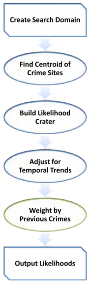
Your team has been asked by a local police agency to develop a method to aid in their investigations of serial criminals. The approach that you develop should make use of at least two different schemes to generate a geographical profile. You should develop a technique to combine the results of the different schemes and generate a useful prediction for law enforcement officers. The prediction should provide some kind of estimate or guidance about possible locations of the next crime based on the time and locations of the past crime scenes. If you make use of any other evidence in your estimate, you must provide specific details about how you incorporate the extra information. Your method should also provide some kind of estimate about how reliable the estimate will be in a given situation, including appropriate warnings.

In addition to the required one-page summary, your report should include an additional two-page executive summary. The executive summary should provide a broad overview of the potential issues. It should provide an overview of your approach and describe situations when it is an appropriate tool and situations in which it is not an appropriate tool. The executive summary will be read by a chief of police and should include technical details appropriate to the intended audience.

(10)

The Results

The solution papers were coded at COMAP headquarters so that names and affiliations of the authors would be unknown to the judges. Each paper was then read preliminarily by two “triage” judges at either Appalachian State University (Sweet Spot Problem) or at the National Security Agency (Crimi- nology Problem). At the triage stage, the summary and overall organization are the basis for judging a paper. If the judges’ scores diverged for a paper, the judges conferred; if they still did not agree, a third judge evaluated the paper.

Additional Regional Judging sites were created at the U.S. Military Academy and at the Naval Postgraduate School to support the growing number of contest submissions.

Final judging took place at the Naval Postgraduate School, Monterey, CA.

The judges classified the papers as follows:

Honorable Successful

Outstanding Finalist Meritorious Mention Participation Total

Sweet Spot Problem 4 5 180 217 533 939

Criminology Problem 5 7 251 325 712 1300

9 12 431 542 1245 2239

We list here the 9 teams that the judges designated as Outstanding; the list of all participating schools, advisors, and results is at the COMAP Website.

Outstanding Teams

Institution and Advisor Team Members

Sweet Spot Problem

“An Optimal Model of ‘Sweet Spot’ Effect”

Huazhong University of Science and Technology

Wuhan, Hubei, China Liang Gao

Zhe Xiong Qipei Mei Fei Han

“The Sweet Spot: A Wave Model of Baseball Bats”

Princeton University Princeton, NJ

Robert Calderbank

Yang Mou Peter Diao Rajib Quabili

(11)

“Brody Power Model: An Analysis of Baseball’s

‘Sweet Spot’”

U.S. Military Academy West Point, NY

Elizabeth Schott

David Covell Ben Garlick

Chandler Williams

“An Identification of ‘Sweet Spot’”

Zhejiang University Hangzhou, China Xinxin Xu

Cong Zhao Yuguang Yang Zuogong Yue

Criminology Papers

“Predicting a Serial Criminal’s Next Crime Location Using Geographic Profiling”

Bucknell University Lewisburg, PA Nathan C. Ryan

Bryan Ward Ryan Ward Dan Cavallaro

“Following the Trail of Data”

Rensselaer Polytechnic Institute Troy, NY

Peter R. Kramer

Yonatan Naamad Joseph H. Gibney Emily P. Meissen

“From Kills to Kilometers: Using Centrographic Techniques and Rational Choice Theory for Geographical Profiling of Serial Killers”

Tufts University Medford, MA Scott MacLachlan

Daniel Brady Liam Clegg Victor Minden

“Centroids, Clusters, and Crime: Anchoring the Geographic Profile of Serial Criminals”

University of Colorado—Boulder Boulder, CO

Anne M. Dougherty

Anil S. Damle Colin G. West Eric J. Benzel

“Tracking Serial Criminals with a Road Metric”

University of Washington Seattle, WA

James Allen Morrow

Ian Zemke Mark Bun Jerry Li

(12)

Awards and Contributions

Each participating MCM advisor and team member received a certificate signed by the Contest Director and the appropriate Head Judge.

INFORMS, the Institute for Operations Research and the Management Sciences, recognized the teams from Princeton University (Sweet Spot Prob- lem) and Tufts University (Criminology Problem) as INFORMS Outstand- ing teams and provided the following recognition:

• a letter of congratulations from the current president of INFORMS to each team member and to the faculty advisor;

• a check in the amount of $300 to each team member;

• a bronze plaque for display at the team’s institution, commemorating team members’ achievement;

• individual certificates for team members and faculty advisor as a personal commemoration of this achievement; and

• a one-year student membership in INFORMS for each team member, which includes their choice of a professional journal plus the OR/MS Today periodical and the INFORMS newsletter.

The Society for Industrial and Applied Mathematics (SIAM) designated one Outstanding team from each problem as a SIAM Winner. The teams were from Huazhong University of Science and Technology (Sweet Spot Problem) and Rensselaer Polytechnic Institute (Criminology Problem). Each of the team members was awarded a $300 cash prize, and the teams received partial expenses to present their results in a special Minisymposium at the SIAM Annual Meeting in Pittsburgh, PA in July. Their schools were given a framed hand-lettered certificate in gold leaf.

The Mathematical Association of America (MAA) designated one Out- standing North American team from each problem as an MAA Winner.

The teams were from the U.S. Military Academy (Sweet Spot Problem) and the University of Colorado—Boulder (Criminology Problem). With partial travel support from the MAA, the teams presented their solution at a special session of the MAA Mathfest in Pittsburgh, PA in August. Each team member was presented a certificate by an official of the MAA Committee on Undergraduate Student Activities and Chapters.

Ben Fusaro Award

One Meritorious or Outstanding paper was selected for each problem for the Ben Fusaro Award, named for the Founding Director of the MCM and awarded for the seventh time this year. It recognizes an especially creative approach; details concerning the award, its judging, and Ben Fusaro are in

(13)

Vol. 25 (3) (2004): 195–196. The Ben Fusaro Award winners were Prince- ton University (Sweet Spot Problem) and Duke University (Criminology Problem). A commentary on the latter appears in this issue.

Judging

Director

Frank R. Giordano, Naval Postgraduate School, Monterey, CA Associate Director

William P. Fox, Dept. of Defense Analysis, Naval Postgraduate School, Monterey, CA

Sweet Spot Problem Head Judge

Marvin S. Keener, Executive Vice-President, Oklahoma State University, Stillwater, OK

Associate Judges

William C. Bauldry, Chair, Dept. of Mathematical Sciences,

Appalachian State University, Boone, NC (Head Triage Judge)

Patrick J. Driscoll, Dept. of Systems Engineering, U.S. Military Academy, West Point, NY (INFORMS Judge)

J. Douglas Faires, Youngstown State University, Youngstown, OH

Ben Fusaro, Dept. of Mathematics, Florida State University, Tallahassee, FL (SIAM Judge)

Michael Jaye, Dept. of Mathematical Sciences, Naval Postgraduate School, Monterey, CA

John L. Scharf, Mathematics Dept., Carroll College, Helena, MT (MAA Judge)

Michael Tortorella, Dept. of Industrial and Systems Engineering, Rutgers University, Piscataway, NJ (Problem Author)

Richard Douglas West, Francis Marion University, Florence, SC Criminology Problem

Head Judge

Maynard Thompson, Mathematics Dept., University of Indiana, Bloomington, IN

Associate Judges

Peter Anspach, National Security Agency, Ft. Meade, MD (Head Triage Judge)

Kelly Black, Mathematics Dept., Union College, Schenectady, NY

(14)

Jim Case (SIAM Judge)

Frank R. Giordano, Naval Postgraduate School, Monterey, CA Veena Mendiratta, Lucent Technologies, Naperville, IL

David H. Olwell, Naval Postgraduate School, Monterey, CA

Michael O’Leary, Towson State University, Towson, MD (Problem Author) Kathleen M. Shannon, Dept. of Mathematics and Computer Science,

Salisbury University, Salisbury, MD (MAA Judge)

Dan Solow, Case Western Reserve University, Cleveland, OH (INFORMS Judge)

Marie Vanisko, Dept. of Mathematics, Carroll College, Helena, MT (Ben Fusaro Award Judge)

Regional Judging Session at U.S. Military Academy Head Judges

Patrick J. Driscoll, Dept. of Systems Engineering,

United States Military Academy (USMA), West Point, NY Associate Judges

Tim Elkins, Dept. of Systems Engineering, USMA Darrall Henderson, Sphere Consulting, LLC

Steve Horton, Dept. of Mathematical Sciences, USMA Tom Meyer, Dept. of Mathematical Sciences, USMA Scott Nestler, Dept. of Mathematical Sciences, USMA Regional Judging Session at Naval Postgraduate School Head Judges

Frank R. Giordano, Naval Postgraduate School, Monterey, CA Associate Judges

Matt Boensel, Robert Burks, Peter Gustaitis, Michael Jaye, and Greg Mislick

—all from the Naval Postgraduate School, Monterey, CA Triage Session for Sweet Spot Problem

Head Triage Judge

William C. Bauldry, Chair, Dept. of Mathematical Sciences, Appalachian State University, Boone, NC

Associate Judges

Jeffry Hirst, Greg Rhoads, and Kevin Shirley

—all from Dept. of Mathematical Sciences, Appalachian State University, Boone, NC

(15)

Triage Session for Criminology Problem Head Triage Judge

Peter Anspach, National Security Agency (NSA), Ft. Meade, MD

Associate Judges Jim Case

Other judges from inside and outside NSA, who wish not to be named.

Sources of the Problems

The Sweet Spot Problem was contributed by Michael Tortorella (Rutgers University), and the Criminology Problem by Michael O’Leary (Towson University) and Kelly Black (Clarkson University).

Acknowledgments

Major funding for the MCM is provided by the National Security Agency (NSA) and by COMAP. Additional support is provided by the Institute for Operations Research and the Management Sciences (INFORMS), the Soci- ety for Industrial and Applied Mathematics (SIAM), and the Mathematical Association of America (MAA). We are indebted to these organizations for providing judges and prizes.

We also thank for their involvement and support the MCM judges and MCM Board members for their valuable and unflagging efforts, as well as

• Two Sigma Investments. (This group of experienced, analytical, and technical financial professionals based in New York builds and operates sophisticated quantitative trading strategies for domestic and international markets. The firm is successfully managing several billion dol- lars using highly-automated trading technologies. For more information about Two Sigma, please visithttp://www.twosigma.com.)

• Jane Street Capital, LLC. (This proprietary trading firm operates around the clock and around the globe. “We bring a deep understanding of markets, a scientific approach, and innovative technology to bear on the problem of trading profitably in the world’s highly competitive financial markets, focusing primarily on equities and equity derivatives. Founded in 2000, Jane Street employes over 200 people in offices in new York, Lon- don, and Tokyo. Our entrepreneurial culture is driven by our talented team of traders and programmers.” For more information about Jane Street Capital, please visithttp://www.janestreet.com.)

(16)

Cautions

To the reader of research journals:

Usually a published paper has been presented to an audience, shown to colleagues, rewritten, checked by referees, revised, and edited by a journal editor. Each paper here is the result of undergraduates working on a problem over a weekend. Editing (and usually substantial cutting) has taken place; minor errors have been corrected, wording altered for clarity or economy, and style adjusted to that of The UMAP Journal. The student authors have proofed the results. Please peruse their efforts in that context.

To the potential MCM Advisor:

It might be overpowering to encounter such output from a weekend of work by a small team of undergraduates, but these solution papers are highly atypical. A team that prepares and participates will have an enrich- ing learning experience, independent of what any other team does.

COMAP’s Mathematical Contest in Modeling and Interdisciplinary Con- test in Modeling are the only international modeling contests in which students work in teams. Centering its educational philosophy on mathematical modeling, COMAP uses mathematical tools to explore real-world problems. It serves the educational community as well as the world of work by preparing students to become better-informed and better-prepared citi- zens.

Editor’s Note

The complete roster of participating teams and results has become too long to reproduce in the printed copy of the Journal. It can now be found at the COMAP Website, in separate files for each problem:

http://www.comap.com/undergraduate/contests/mcm/contests/

2010/results/2010_MCM_Problem_A.pdf

http://www.comap.com/undergraduate/contests/mcm/contests/

2010/results/2010_MCM_Problem_B.pdf

(17)

The Sweet Spot: A Wave Model of Baseball Bats

Rajib Quabili Peter Diao Yang Mou

Princeton University Princeton, NJ

Advisor: Robert Calderbank

Abstract

We determine the sweet spot on a baseball bat. We capture the essential physics of the ball–bat impact by taking the ball to be a lossy spring and the bat to be an Euler-Bernoulli beam. To impart some intuition about the model, we begin by presenting a rigid-body model. Next, we use our full model to reconcile various correct and incorrect claims about the sweet spot found in the literature. Finally, we discuss the sweet spot and the performances of corked and aluminum bats, with a particular emphasis on hoop modes.

Introduction

Although a hitter might expect a model of the bat–baseball collision to yield insight into how the bat breaks, how the bat imparts spin on the ball, how best to swing the bat, and so on, we model only the sweet spot.

There are at least two notions of where the sweet spot should be—an impact location on the bat that either

• minimizes the discomfort to the hands, or

• maximizes the outgoing velocity of the ball.

We focus exclusively on the second definition.

The velocity of the ball leaving the bat is determined by

• the initial velocity and rotation of the ball,

• the initial velocity and rotation of the bat,

(18)

• the relative position and orientation of the bat and ball, and

• the force over time that the hitter’s hands applies on the handle.

We assume that the ball is not rotating and that its velocity at impact is perpendicular to the length of the bat. We assume that everything occurs in a single plane, and we will argue that the hands’ interaction is negligible.

In the frame of reference of the center of mass of the bat, the initial conditions are completely specified by

• the angular velocity of the bat,

• the velocity of the ball, and

• the position of impact along the bat.

The location of the sweet spot depends not on just the bat alone but also on the pitch and on the swing.

The simplest model for the physics involved has the sweet spot at the center of percussion [Brody 1986], the impact location that minimizes discom- fort to the hand. The model assumes the ball to be a rigid body for which there are conjugate points: An impact at one will exactly balance the angular recoil and linear recoil at the other. By gripping at one and impacting at the other (the center of percussion), the hands experience minimal shock and the ball exits with high velocity. The center of percussion depends heavily on the moment of inertia and the location of the hands. We cannot accept this model because it both erroneously equates the two definitions of sweet spot and furthermore assumes incorrectly that the bat is a rigid body.

Another model predicts the sweet spot to be between nodes of the two lowest natural frequencies of the bat [Nathan 2000]. Given a free bat al- lowed to oscillate, its oscillations can be decomposed into fundamental modes of various frequencies. Different geometries and materials have different natural frequencies of oscillation. The resulting wave shapes suggest how to excite those modes (e.g., plucking a string at the node of a vibrational mode will not excite that mode). It is ambiguous which definition of sweet spot this model uses. Using the first definition, it would focus on the uncomfortable excitations of vibrational modes: Choosing the impact location to be near nodes of important frequencies, a minimum of uncomfortable vibrations will result. Using the second definition, the worry is that energy sent into vibrations of the bat will be lost. This model assumes that the most important energies to model are those lost to vibration.

This model raises many questions. Which frequencies get excited and why? The Fourier transform of an impulse in general contains infinitely many modes. Furthermore, wood is a viscoelastic material that quickly dissipates its energies. Is the notion of an oscillating bat even relevant to modeling a bat? How valid is the condition that the bat is free? Ought the system be coupled with hands on the handle, or the arm’s bone structure, or possibly even the ball? What types of oscillations are relevant? A cylin-

(19)

drical structure can support numerous different types of modes beyond the transverse modes usually assumed by this model [Graff 1975].

Following the center-of-percussion line of reasoning, how do we model the recoil of the bat? Following the vibrational-nodes line of reasoning, how do we model the vibrations of the bat? In the general theory of impact mechanics [Goldsmith 1960], these two effects are the main ones (assuming that the bat does not break or deform permanently). Brody [1986] ignores vibrations, Cross [1999] ignores bat rotation but studies the propagation of the impulse coupled with the ball, and Nathan [2000] emphasizes vibrational modes. Our approach reconciles the tension among these approaches while emphasizing the crucial role played by the time-scale of the collision.

Our main goal is to understand the sweet spot. A secondary goal is to understand the differences between the sweet spots of different bat types.

Although marketers of bats often emphasize the sweet spot, there are other relevant factors: ease of swing, tendency of the bat to break, psychological effects, and so on. We will argue that it doesn’t matter to the collision whether the batter’s hands are gripping the handle firmly or if the batter follows through on the swing; these circumstances have no bearing on the technique required to swing the bat or how the bat’s properties affect it.

Our paper is organized as follows. First, we present the Brody rigid- body model, illuminating the recoil effects of impact. Next we present a full computational model based on wave propagation in an Euler-Bernoulli beam coupled with the ball modeled as a lossy spring. We compare this model with others and explore the local nature of impact, the interaction of recoil and vibrations, and robustness to parameter changes. We adjust the parameters of the model to comment on the sweet spots of corked bats and aluminum bats. Finally, we investigate the effect of hoop frequencies on aluminum bats.

A Simple Example

We begin by considering only the rigid recoil effects of the bat–ball collision, much as in Brody [1986]. For simplicity, we assume that the bat is perfectly rigid. Because the collision happens on such a short time-scale (around 1 ms), we treat the bat as a free body. That is to say, we are not concerned with the batter’s hands exerting force on the bat that may be transferred to the ball.

The bat has massM and moment of inertiaI about its center of mass.

From the reference frame of the center of mass of the bat just before the collision, the ball has initial velocityv_iin the positivex-direction while the bat has initial angular velocity ωi. In our setup, vi and ωi have opposite signs when the batter is swinging at the ball as in Figure 1, in which arrows point in the positive directions for the corresponding parameters.

(20)

Figure 1. The collision.

The ball collides with the bat at a distance l from the center of mass of the bat.

We assume that the collision is head-on and view the event such that all they-component velocities are zero at the moment of the collision. After the collision, the ball has a final velocityvf and the bat has a final linear velocity Vf and an angular velocityωf at the center of mass.

When the ball hits the bat, the ball briefly compresses and decompresses, converting kinetic energy to potential energy and back.

However, some energy is lost in the process, that is, the collision is inelastic. The ratio of the relative speeds of the bat and the ball before and after the collision is known as the coefficient of restitution, customarily des- ignated by e: e = 0 represents a perfectly inelastic collision, and e = 1 means a perfectly elastic one. In this basic model, we make two simplifying assumptions:

• eis constant along the length of the bat, and

• eis constant for allvi.

Given our pre-collision conditions, we can write:

Conservation of linear momentum:

M Vf = m(vi− v^f) Conservation of angular momentum:

I(ωf − ωⁱ) = ml(vi− v^f), Definition of the coefficient of restitution:

e(v_i− ωil) = −vf + V_f + w_fl.

Solving forvf gives

vf = −vⁱ(e − _M^m∗) + ωil(1 + e) 1 + _M^m_∗ , where

M^∗ = M 1 + ^{M l}_I² is the effective mass of the bat.

(21)

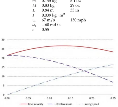
For calibration purposes, we use the following data, which are typical of a regulation bat connecting with a fastball in Major League Baseball. The results are plotted in Figure 2.

m 0.145 kg 5.1 oz

M 0.83 kg 29 oz

L 0.84 m 33 in

I 0.039 kg_·m²

v_i 67 m/s 150 mph

ω_i −60 rad/s e 0.55

Figure 2. Final velocity vf (solid arc at top), swing speed ωil(dotted rising line), and effective mass (dashed falling curve) as a function of distance l (in meters) from center of mass.

The maximum exit velocity is 27 m/s, and the sweet spot is 13 cm from the center of mass. Missing the sweet spot by up to 5 cm results in at most 1 m/s difference from the maximum velocity, implying a relatively wide sweet spot.

From this example, we see that the sweet spot is determined by a mul- titude of factors, including the length, mass, and shape of the baseball bat;

the mass of the baseball; and the coefficient of restitution between bat and ball. Furthermore, the sweet spot is not uniquely determined by the bat and ball: It depends also on the incoming baseball speed and the batter’s swing speed.

Figure 2 also shows intuitively why the sweet spot is located somewhere between the center of mass and the end of the barrel. As the point of collision moves outward along the bat, the effective mass of the bat goes up, so that a greater fraction of the initial kinetic energy is put into the bat’s rotation.

At the same time, the rotation in the bat means that the barrel of the bat is moving faster than the center of mass (or handle). These two effects work in opposite directions to give a unique sweet spot that’s not at either endpoint.

(22)

However, this model tells only part of the story. Indeed, some of our starting assumptions contradict each other:

• We treated the bat as a free body because the collision time was so short.

In essence, during the 1 ms of the collision, the ball “sees” only the local geometry of the bat, not the batter’s hands on the handle. On the other hand, we assumed that the bat was perfectly rigid—but that means that the ball “sees” the entire bat.

• We also assumed that e is constant along the length of the bat and for different collision velocities. Experimental evidence [Adair 1994] sug- gests that neither issue can be ignored for an accurate prediction of the location of the sweet spot.

We need a more sophisticated model to address these shortcomings.

Our Model

We draw from Brody’s rigid-body model but more so from Cross [1999].

One could describe our work as an adaptation of Cross’s work to actual baseball bats. Nathan [2000] attempted such an adaptation but was misled by incorrect intuition about the role of vibrations. We describe his approach and error as a way to explain Cross’s work and to motivate our work.

Previous Models

Brody’s rigid-body model correctly predicts the existence of a sweet spot not at the end of the bat. That model suffers from the fact that the bat is not a rigid body and experiences vibrations. One way to account for vibrations is to model the bat as a flexible object. Beam theories (of varying degrees of accuracy and complication) can model a flexible bat. Van Zandt [1992] was the first to carry out such an analysis, modeling the beam as a Timoshenko beam, a fourth-order theory that takes into account both shear forces and tensile stresses. The equations are complicated and we will not need them.

Van Zandt’s model assumes the ball to be uncoupled from the beam and simply takes the impulse of the ball as a given. The resulting vibrations of the bat are used to predict the velocity of the beam at the impact point (by summing the Brody velocity with the velocity of the displacement at the impact point due to vibrations) and thence the exit velocity of the ball from the equations of the coefficient of restitution [van Zandt 1992].

Cross [1999] modeled the interaction of the impact of a ball with an aluminum beam, using the less-elaborate Euler-Bernoulli equations to model the propagation of waves. In addition, he provided equations to model the dynamic coupling of the ball to the beam during the impact. After discretizing the beam spatially, he assumed that the ball acts as a lossy spring coupled to the single component of the region of impact.

(23)

Cross’s work was motivated by both tennis rackets and baseball bats, which differ importantly in the time-scale of impact. The baseball bat’s colli- sion lasts only about 1 ms, during which the propagation speed of the wave is very important. In this local view of the impact, the importance of the baseball’s coupling with the bat is increased.

Cross argues that the actual vibrational modes and node points are largely irrelevant because the interaction is localized on the bat. The boundary conditions matter only if vibrations reflect off the boundaries; an impact not close enough to the barrel end of the bat will not be affected by the boundary there. In particular, a pulse reflected from a free boundary returns with the same sign (deflected away from the ball, decreasing the force on the ball, decreasing the exit velocity), but a pulse reflected from a fixed boundary returns with the opposite sign (deflected towards the ball, pushing it back, increasing the exit velocity). Away from the boundary, we expect the exit velocity to be uniform along a non-rotating bat. Cross’s model predicts all of these effects, and he experimentally verified them. In our model, we expect similar phenomena, plus the narrowing of the barrel near the handle to act somewhat like a boundary.

Nathan’s model also attempted to combine the best features of Van Zandt and Cross [Nathan 2000]. His theory used the full Timoshenko theory for the beam and the Cross model for the ball. He even acknowledged the local nature of impact. So where do we diverge from him? His error stems from an overemphasis on trying to separate out the ball’s interaction with each separate vibrational mode.

The first sign of inconsistency comes when he uses the “orthogonality of the eigenstates” to determine how much a given impulse excites each mode. The eigenstates are not orthogonal. Many theories yield symmetric matrices that need to be diagonalized, yielding the eigenstates; but Tim- oshenko’s theory does not, due to the presence of odd-order derivatives in its equations. Nathan’s story plays out beautifully if only the eigenstates were actually orthogonal; but we have numerically calculated the eigenstates, and they are not even approximately orthogonal. He uses the orthogonality to draw important conclusions:

• The location of the nodes of the vibrational modes are important.

• High-frequency effects can be completely ignored.

We disagree with both of these.

The correct derivation starts with the following equation of motion, wherekis the position of impact,yiis the displacement andFiis the external force on theith segment of the bat, andH_ij is an asymmetric matrix:

y⁰⁰_k(t) = Hkjyj(t) + Fk(t).

We write the solutions as yk(t) = Φknan(t), where the rows of Φkn are eigenmodes with eigenvalues−ωn². Explicitly,HjkΦkn = −ωn²Φjn, andΦkn

(24)

indicates the kth component of the nth eigenmode. Then we write the equation of motion:

Φkna⁰⁰_n(t) + Φknω_n²an(t) = Fk = ΦknΦ⁻¹_njFj, a⁰⁰_n(t) + ω_n²a_n(t) = Φ⁻¹_nkF_k.

In the last step, we used the fact that the eigenmodes form a complete basis.

Nathan’s paper uses on the right-hand side simply ΦknFk scaled by a normalization constant. At first glance, this seems like a minor technical detail, but the physics here is important. We calculate that theΦ⁻¹_nkF_k terms stay fairly large for even high values ofn, corresponding to the high- frequency modes (k is just the position of the impact). This means that there are significant high-frequency components, at least at first. In fact, the high-frequency modes are necessary for the impulse to propagate slowly as a wave packet. In Nathan’s model, only the lowest standing modes are excited; so the entire bat starts vibrating as soon as the ball hits. This contradicts his earlier belief in localized collision (which we agree with), that the collision is over so quickly that the ball “sees” only part of the bat. Nathan also claims that the sweet spot is related to the nodes of the lowest mode, which contradicts locality: The location of the lowest-order nodes depends on the geometry of the entire bat, including the boundary conditions at the handle.

While the inconsistencies in the Nathan model may cancel out, we build our model on a more rigorous footing. For simplicity, we use the Euler- Bernoulli equations rather than the full Timoshenko equations. The difference is that the former ignore shear forces. This should be acceptable;

Nathan points out that his model is largely insensitive to the shear modulus. We solve the differential equations directly after discretizing in space rather than decomposing into modes. In these ways, we are following the work of Cross [1999].

On the other hand, our model extends Cross’s work in several key ways:

• We examine parameters much closer to those relevant to baseball. Cross’s models focused on tennis, featuring an aluminum beam of width 0.6 cm being hit with a ball of 42 g at around 1 m/s. For baseball, we have an aluminum or wood bat of radius width 6 cm being hit with a ball of 145 g traveling at 40 m/s (which involves 5,000 times as much impact energy).

• We allow for a varying cross-section, an important feature of a real bat.

• We allow the bat to have some initial angular velocity. This will let us scrutinize the rigid-body model prediction that higher angular velocities lead to the maximum power point moving farther up the barrel.

To reiterate, the main features of our model are

• an emphasis on the ball coupling with the bat,

(25)

• finite speed of wave propagation in a short time-scale, and

• adaptation to realistic bats.

These are natural outgrowths of the approaches in the literature.

Mathematics of Our Model

Our equations are a discretized version of the Euler-Bernoulli equations:

ρ ∂²y(z, t)

∂t² = F (z, t) + ∂²

∂z² µ

Y I ∂²y(z, t)

∂z²

∂ ,

where

ρ is the mass density, y(z, t) is the displacement,

F (z, t) is the external force (in our case, applied by the ball), Y is the Young’s modulus of the material (a constant), and I is the second moment of area (πR⁴/4for a solid disc).

We discretizezin steps of∆. The only force is from the ball, in the negative direction to thekth segment. Our discretized equation is:

ρA∆d²yi

dt² = −δ^ikF (t) − Y

∆³

∑

I_i−1(y_i−2 − 2yi−1 + yi)

−2Ii(y_i−1 − 2yi+ y_i+1) + I_i+1(y_i− 2yi+1+ y_i+2)

∏ . Our dynamic variables arey1 throughyN. For a fixed left end, we pretend thaty₋₁ = y0 = 0. For a free left end, we pretend that

y1 − y⁰ = y0− y−1 = y₋₁− y−2.

The conditions on the right end are analogous. These are the same conditions that Cross uses.

Finally, we have an additional variable for the ball’s position (relative to some zero point)w(t). Initially,w(t)is positive andw⁰(t)is negative, so the ball is moving from the positive direction towards the negative. Letu(t) = w(t) − y^k(t). This variable represents the compression of the ball, and we replaceF (t)withF°

u(t), u⁰(t)¢

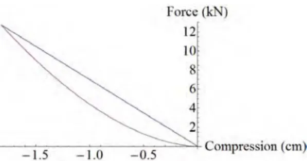
. Initially,u(t) = 0andu⁰(t) = −v^ball^{. The} force between the ball and the bat takes the form of hysteresis curves such as the ones shown in Figure 3.

(26)

Figure 3. A hysteresis curve used in our modeling, with maximum compression 1.5 cm.

The higher curve is taken whenu⁰(t) < 0(compression) and the lower curve when u⁰(t) > 0 (expansion). When u(t) > 0, the force is zero. The equation of motion for the ball is then

w⁰⁰(t) = u⁰⁰(t) + y⁰⁰_k(t) = F°

u(t), u⁰(t)¢ . We have eliminated the variablew.

We have yet to specify the functionF°

u(t), u⁰(t)¢

. As can be seen in videos [Baseball Research Center n.d.], the ball compresses significantly (often more than 1 cm) in a collision. The compression and decompression is lossy. We could model this loss by subtracting a fraction of the ball’s energy after the collision; that approach is good enough for many purposes, but we instead follow Nathan and use a nonlinear spring with hysteresis.

Since W = R

F dx, the total energy lost is the area between the two curves in Figure 3. A problem with creating hysteresis curves is that one does not know the maximum compression (i.e., where to start drawing the bottom curve) until after solving the equations of motion. In practice, we solve the equation in two steps.

The main assumptions of our model derive from the main assumptions of each equation:

• The first is the exact form of the hysteresis curve of the ball. Cross [1999]

argues that the exact form of the curve is not very important as long as the duration of impact, magnitude of impulse, maximum compression of the ball, and energy loss are roughly correct.

• Both the Timoshenko and Euler-Bernoulli theories ignore azimuthal and longitudinal waves. This is a fundamental assumption built into all of the approaches in the literature. Assuming that the impact of the ball is transverse and the ball does not rotate, the assumption is justified.

The assumptions of our models are the same as those in the literature, so they are confirmed by the literature’s experiments.

(27)

Simulation and Analysis

Simulation Results

Our model’s two main features are wave propagation in the bat and nonlinear compression/decompression of the ball. The latter is illustrated by the asymmetry of the plot in Figure 4a. This plot also reveals the time- scale of the collision: The ball leaves the bat 1.4 ms after impact. During and after collision, shock waves propagate through the bat.

In this example, the bat was struck 60 cm from the handle. What does the collision look like at 10 cm from the handle? Figure 4b shows the answer:

The other end of the bat does not feel anything until about 0.4 ms and does not feel significant forces until about 1.0 ms. By the time that portion of the bat swings back (almost 2.0 ms), the ball has already left contact with the bat. This illuminates an important point: We are concerned only with forces on the ball that act within the 1.4 ms time-frame of the collision. Any waves taking longer to return to the impact location do not affect exit velocity.

Figure 4.

a. Left: The force between the ball and the bat as a function of time; the impulse lasts 1.4 ms.

b. Right: The waveform of y10(t)when the bat is struck at 60 cm. The impulse reaches this chunk at around 0.4 ms but does not start moving significantly until later.

Having demonstrated the basic features of our model, we now replicate some of Cross’s results but with baseball-like parameters. In Figure 5a, we show that the effects of fixed- vs. free-boundary conditions are in agreement with Cross’s model.

As we expected, fixed boundaries enhance the exit velocity and free boundaries reduce them. From this result, we see the effect of the shape of the bat. The handle does indeed act like a free boundary. The distance between the boundaries is too small to get a flat zone in the exit velocity vs.

position curve. If we extend the barrel by 26 cm, a flat zone develops (Fig- ure 5b; notice the change in axes). Intuitively, this flat zone exists because the ball “sees” only the local geometry of the bat and the boundaries are too far away to have a substantial effect.

From now on, we use an 84-cm bat free on both ends, where position zero denotes the handle end. In this base case, the sweet spot is at 70 cm. We

(28)

Figure 5.

a. Left: Exit velocity vs. impact position for a free boundary (solid line) and for a fixed boundary (dashed line), with barrel end fixed but handle end free, for an 84-cm bat

b. Right: The same graph for a free 110-cm bat.

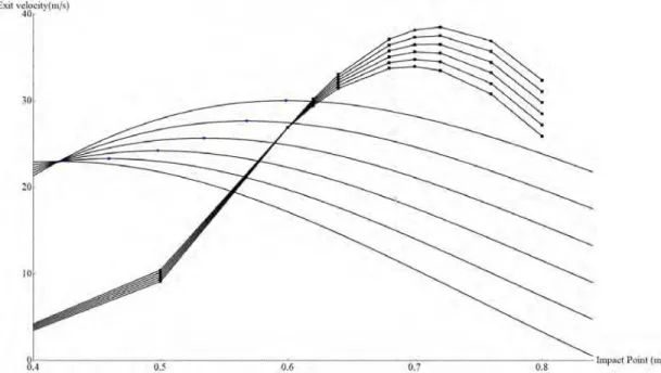
investigate the dependence of the exit speed on the initial angular velocity.

According to rigid-body models, the sweet spot is exactly at the center of mass if the bat has no angular velocity. In Figure 6, we present the results of changing the angular velocity. Our results contrast greatly with the simple example presented earlier. While the angular-rotation effect is still there, the effective mass plays only a negligible role in determining the exit speed.

In other words, the bat is not a rigid body because the entire bat does not react instantly. The dominating effect is from the boundaries: the end of the barrel and where the barrel tapers off. These free ends cause a significant drop in exit velocity. Increasing the angular velocity of the bat increases the exit velocity, in part just because the impact velocity is greater (by a factor ofωi times the distance from the center of mass of the bat).

Figure 6. Exit velocity vs. impact position at various initial angular velocities of the bat. Our model predicts the solid curves, while the dashed lines represent the simple model. The dots are at the points where Brody’s solution is maximized.

(29)

In Figure 7a, we show that near the sweet spot (at 0.7 m), increasing angular velocity actually decreases the excess exit velocity (relative to the impact velocity). We should expect this, since at higher impact velocity, more energy is lost to the ball’s compression and decompression. To con- firm this result, we also recreate the plot in Figure 7b but without the hysteresis curve—in which case this effect disappears. This example is one of the few places where the hysteresis curve makes a difference, confirm- ing experimental evidence [Adair 1994; Nathan 2003] that the coefficient of restitution decreases with increasing impact velocity.

Figure 7.

Exit velocity minus impact velocity vs. impact position, for initial angular velocities of the bat.

a. Left: Near the center of mass, higher angular velocity gives higher excess exit velocity, but towards the sweet spot the lines cross and higher angular velocity gives lower excess exit velocity.

b. Right: The same plot without a hysteresis curve. The effect disappears.

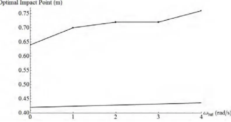
The results for angular velocity contrast with the simple model. As evident from Figure 8, the rigid-body model greatly overestimates this effect for large angular velocities.

,

Figure 8. Optimal impact position vs. angular velocity. The straight line is the rigid-body predic- tion, while the points are our model’s prediction.

Parameter Space Study

There are various adjustable parameters in our model. For the bat, we use densityρ = 649kg/m³and Young’s modulusY = 1.814 × 10¹⁰^N/m²^.

(30)

Figure 9. The profile of our bat.

These values, as well as our bat profile (Figure 9), were used by Nathan as typical values for a wooden bat. While these numbers are in good agreement with other sources, we will see that these numbers are fairly special.

As a result of our bat profile, the mass is 0.831 kg and the moment of inertia around the center of mass (at 59.3 cm from the handle of our 84 cm bat) is 0.039 kg·^m². We let the 145-g ball’s initial velocity be 40 m/s, and set up our hysteresis curve so that the compression phase is linear with spring constant7 × 10⁵ ^N/m.

• We vary the density of the bat and see that the density value occupies a narrow region that gives peaked exit-velocity curves (see Figure 10).

Figure 10.

Exit velocity vs. impact position for various densities. The solid line is the original ρ = 649kg/m³. a. Left: Dotted is ρ = 700, dashed is ρ = 1000. b. Right: Dotted is ρ = 640, dashed is ρ = 500.

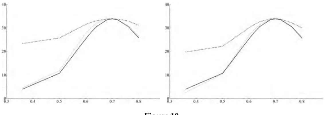
• We also vary the Young’s modulus and shape of bat to similar effect (see Figure 11). The fact that varying any of Nathan’s parameters makes the resulting exit velocity vs. location plot less peaked means that baseball bats are specially designed to have the shape shown in Figure 9 (or else the parameters were picked in a special way).

• Finally, we varyy, the speed of the ball (see Figure 12). The exit velocity simply scales with the input velocity, as expected.

Alternatives to Wooden Bats

Having checked the stability of our model for small parameter changes, we now change the parameters drastically, so as to model corked and aluminum bats.

(31)

Figure 11.

a. Left: Varying the value of Y . Solid is Y = 1.1814 × 10¹⁰N/m²; dashed is 1.25 times as much, while dotted is 0.8 times.

b. Right: Varying the shape of the bat. Solid is the original shape; dashed has a thicker handle region, while dotted has a narrower handle region.

Figure 12. Varying the speed of the ball. Solid is the original 40 m/s, dashed is 50 m/s, while dotted is 30 m/s.

Corked Bat

We model a corked bat as a wood bat with the barrel hollowed out, leaving a shell 1 cm or 1.5 cm thick. The result is shown in Figure 13a.

The exit velocities are higher, but this difference is too small to be taken seriously. This result agrees with the literature: The only advantages of a corked bat are the changes in mass and in moment of inertia.

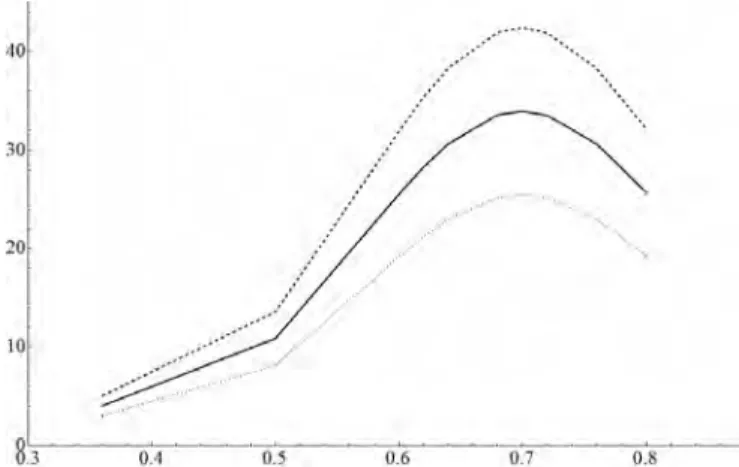
Aluminum Bat

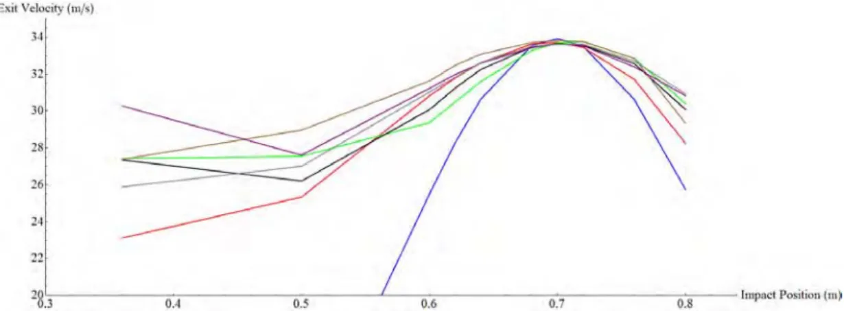
We model an aluminum bat as a 0.3 cm-thick shell with a density of 2700 kg/m³ and Young’s modulus 6.9 × 10¹⁰ ^N/m². The aluminum bat performs much better than the wood bat (Figure 13b). It has the same sweet spot (70 cm) and similar sweet-spot performance, but the exit velocity falls off more gradually away from the sweet spot.

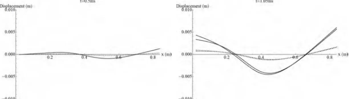
To gain more insight, we animated the displacement of the bat vs. time;

we present two frames of the animation in Figure 14. The aluminum bat is

(32)

Figure 13. Exit velocity vs. distance of point of collision on the bat from the handle end.

a. Corked bat. b. Aluminum bat.

displaced less (absorbing less energy). More importantly, in the right-hand diagram of Figure 14, the curve for the wood bat is still moving down and left, while the aluminum bat’s curve is moving left and pushing the ball back up. The pulse in the aluminum bat travels faster and returns in time to give energy back to the ball. By the time the pulse for the wood bat returns to the impact location, the ball has already left the bat.

Figure 14. Plots of the displacement of an aluminum bat (dashed) and wood bat (solid) being hit by a ball 60 cm from the handle end. The diagram on the right shows two frames superimposed (t = 1.05 ms and t = 1.10 ms) so as to show the motion. The rigid translation and rotation has been removed from the diagrams.

In the literature, the performance of aluminum bats is often attributed to a “trampoline effect,” in which the bat compresses on impact and then springs back before the end of the collision [Russell 2003]. This effect would improve aluminum-bat performance further. The trampoline effect involves exciting so-called “hoop modes,” modes with an azimuthal dependence, which our model cannot simulate directly. For an aluminum bat, one could conceivably use wave equations for a cylindrical sheet (adjusting for the changing radius) and then solve the resulting partial differential equations in three variables. Analysis of such a complex system of equations is beyond the scope of this paper.

Instead, we artificially insert a hoop mode by hanging a mass from a spring at the spot of the bat where the ball hits. We expect the important