水溶液環境原子力顯微鏡系統之設計與開發

(1)

國立臺灣大學工學院機械工程學研究所博士論文

Department of Mechanical Engineering College of Engineering

National Taiwan University Ph.D. Dissertation

水溶液環境原子力顯微鏡系統之設計與開發

Design and Development of Atomic Force Microscope Systems for Liquid Environment

廖先順

Hsien-Shun Liao

指導教授：黃光裕博士

Advisor: Kuang-Yuh Huang, Dr.-Ing.

中華民國 102 年 1 月

January, 2013

(2)

誌謝

在博士班的這段時間中，除了感謝黃光裕老師在論文上的指導外，也給學生參與執行研究計劃的機會，拓展了學生的視野與經驗。感謝中研院物理所的張嘉升、黃英碩老師，除了老師們的真知灼見給予學生許多的啟發與學習，更營造了一個可讓學生們成長發揮的研究環境。

紹剛、志文、恩德、彥甫、仰山、博景學長，謝謝學長們無私的指導與照顧，

給我上課所學不到的寶貴的經驗。原力精密儀器的合作團隊，貴銘、嘉宜、志憲、

敬凱、彥名、建男、育琛、翰弘..，與各位一同開發儀器的時光既充實又有趣。

中研院的同事們：韋僑、韋誠、伯彥、子銘、書正、士嶔、君岳、立維、偉文、

信宏、仕修、秉翔、鑑元、旭佑、曉琪、欣純、奕賢、雅綾、淵智、延松、莉穎、

少傑、崇開、賢真、維哲..，很榮幸能有機會與你們共事、讓我獲益良多。產學團隊與台大的同學們：偉珉、敬修、彥宏、仁峰、宣富、天仁、奕伸、彥名、秉彤、揚文、Chris、Jens、銘延、仲翔、明山..，小至尋找六角板手，大至論文檔案救援都受你們照顧了。謝謝物理所精工室團隊總是幫助我們製作出品質優良的工件。要感謝的人太多無法盡列，願相關的研究者也能從此論文中得到一點助益。

感謝我所信的神，讓我在研究過程中學習謙卑，重新認識自己的所是、所知、

所能之渺小與有限，願榮耀歸與我神。

When I applied my mind to know wisdom and to observe man’s labor on earth – his eyes not seeing sleep day or night – then I saw all that God has done. No one can comprehend what goes on under the sun. Despite all his efforts to search it out, man cannot discover its meaning. Even if a wise man claims he knows, he cannot really comprehend it.

ECCLESIASTES 8:16~17

(3)

摘要

在水溶液環境中之操作能力為原子力顯微鏡的重要優勢之ㄧ，此優點使原子力顯微鏡廣泛地被應用於生化研究的領域。然而，水溶液介質會嚴重影響微懸臂探針之動態特性，進而增加取得高解析與穩定影像的困難度。

在此篇論文中，分別探討微懸臂探針之幾何造型、激振機構、以及像散式偵測方法以改善在水溶液中之性能。考慮微懸臂尺寸，等比例減小微懸臂長度與厚

度可提高 Q 值與共振頻率。此外，相較於微懸臂第一共振模態，高階共振模態可

提供較高之質量靈敏度。在激振機構方面，開發之微懸臂夾持針座可有效減低水中之雜峰，並能提供彎曲式以及扭曲式兩種不同激振模式。藉由光路的修改，像散式偵測系統之靈敏度可被最佳化，並提高光學掃描模式對生物細胞成像之解析度。

最後，應用以上經驗開發一像散式偵測之水溶液原子力顯微鏡系統，水中雜

峰可低於真實微懸臂共振峰值之26.0%。此外，藉由達到對石墨單原子層台階以及

DNA 樣品於水溶液中成像，驗證系統解析度以及量測軟性生物樣品之能力。

關鍵字：原子力顯微鏡、水溶液環境、像散效應

(4)

Abstract

The ability to operate in liquid environment is a remarkable advantage of the atomic force microscope (AFM). This advantage enables the AFM to be applied to the bio-chemical field widely. However, the dynamic properties of the cantilever tip are influenced significantly in liquid, and cause the difficulty in getting high resolution and stable images.

In this dissertation, the cantilever geometry, the excitation mechanism, and the astigmatic detection method are studied for improving the AFM’s performance in liquid.

Considering the cantilever dimensions, the resonant frequency and the Q-factor can be raised through decreasing cantilever thickness and length proportionally. Besides, the high-order resonances can provide higher mass sensitivity than the fundamental one. In the excitation mechanism, a clamp-modification holder is developed for reducing spurious peaks and enhancing the real resonant peak, and provides a more apparent flexural or torsional excitation. Moreover, the sensitivity of the astigmatic detection system is optimized, and the resolution of the optical scanning method is also improved for imaging the bio-sample.

Accumulating the experience above, a liquid-AFM system is developed based on the astigmatic detection method. The spurious peaks are suppressed down to 26.0 % of the resonant peaks in the liquid environment. Furthermore, it is verified that the liquid-AFM can realize high-resolution scanning images of the sub-nano scale graphite layer and the soft DNA sample in water.

Keywords: AFM, Liquid environment, Astigmatism

(5)

List of Figures

Fig. 1.1 Scheme of STM ... 3

Fig. 1.2 First AFM setup ... 4

Fig. 1.3 Biological images of (a) double-stranded DNA (BlueScript II), (b) human blood protein fibrinogen (image size is 450 nm × 450 nm), (c) white blood cell (image size is 9.1 μm × 9.1 μm) ... 5

Fig. 1.4 Force-displacement curve of contact mode ... 7

Fig. 1.5 Force-displacement curves of tapping mode ... 9

Fig. 1.6 Cantilever resonant modes ... 10

Fig. 1.7 Spectra of different length cantilevers ... 12

Fig. 1.8 Two different transmissive ways ... 13

Fig. 2.1 Force sensing system, actuator system, and control system ... 16

Fig. 2.2 SEM images of commercial cantilevers (MikroMasch) ... 17

Fig. 2.3 Double tips artifact ... 18

Fig. 2.4 Scheme of piezoelectric actuator excitation ... 19

Fig. 2.5 Scheme of magnetic excitation method ... 20

Fig. 2.6 Scheme of Lorentz force excitation method ... 20

Fig. 2.7 Scheme of photothermal excitation method ... 21

Fig. 2.8 Cantilever holder design of Asakawa and Fukuma ... 22

Fig. 2.9 Excitation spectrum comparison between two materials ... 23

Fig. 2.10 Cantilever detection methods ... 24

Fig. 2.11 Piezoelectric scanner ... 26

Fig. 2.12 Piezoelectric hysteresis with different input amplitudes ... 27

(9)

Fig. 2.13 AFM images of calibration grating with 3 μm pitch ... 28

Fig. 2.14 Open-loop scanner calibration ... 29

Fig. 2.15 Closed-loop scanner control ... 30

Fig. 2.16 Digital lock-in amplifier diagram ... 32

Fig. 2.17 Z-axis feedback control diagram ... 33

Fig. 2.18 XY-axes scanning control ... 34

Fig. 3.1 Cantilever properties versus cantilever dimensions ... 40

Fig. 3.2 Cantilever properties with L/h = 100 and b = 5 μm ... 41

Fig. 3.3 Cantilever No.02 with different widths ... 42

Fig. 3.4 Cantilever properties versus cantilever width in water... 44

Fig. 3.5 Cantilever No.02 with different lengths ... 45

Fig. 3.6 Dynamic properties versus cantilever length in water ... 45

Fig. 3.7 Modified cantilever with different hole layouts ... 47

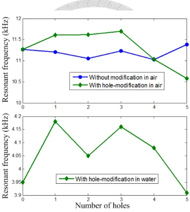
Fig. 3.8 Resonant frequency versus number of holes ... 48

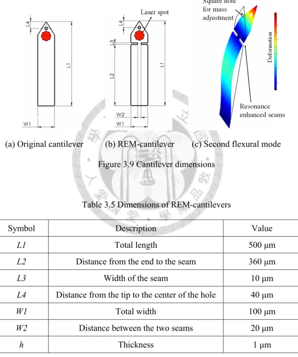
Fig. 3.9 Cantilever dimensions ... 50

Fig. 3.10 Resonant frequency shift Δf versus mass variation Δm ... 52

Fig. 3.11 Configuration of experimental setup ... 53

Fig. 3.12 Modified cantilevers with mass variations ... 54

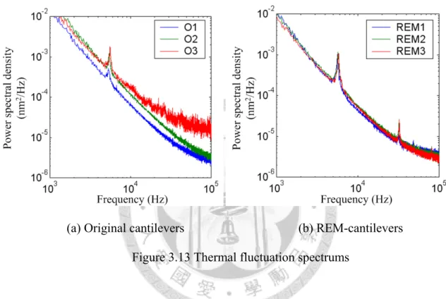
Fig. 3.13 Thermal fluctuation spectrums ... 55

Fig. 3.14 Thermal fluctuation spectra of nth flexural deflection with and without mass-tuning (a) in air and (b) in water ... 58

Fig. 3.15 Experimental and simulated mass sensitivity of five flexura modes in water…. ... 59

(10)

Fig. 4.1 Commercial TR-mode holder ... 63

Fig. 4.2 Spectrums of cantilever PPP-NCHAuD ... 65

Fig. 4.3 Spectrums of cantilever CSC38B ... 67

Fig. 4.4 PEEK-based holder ... 69

Fig. 4.7 Steel-based holder ... 72

Fig. 4.10 Adjustable preload holder ... 75

Fig. 4.11 Spectrums of cantilever PPP-NCHAuD with different preload ... 77

Fig. 4.12 Spectrums of cantilever CSC38B with different preload ... 78

Fig. 4.13 Clamp-modification holder ... 80

Fig. 5.1 (a) Configuration of ADS and (b) focus error signal UFES versus cantilever displacement ... 85

Fig. 5.2 Astigmatic pickup head ... 86

Fig. 5.3 Optical paths of (a) DVD optical disc, and (b) water environment ... 88

Fig. 5.4 ADS sensitivity measurement setup ... 89

Fig. 5.5 UFES versus displacement curves (S-curves) ... 91

Fig. 5.6 Sensitivity SADS versus water thickness hwater ... 92

Fig. 5.7 UFES versus displacement curves (S-curves) ... 93

Fig. 5.8 Optical scanning images of MCF-7 breast cancer cell ... 95

Fig. 5.9 (a) Configuration and (b) construction of calibration setup ... 98

(11)

Fig. 5.10 SEM images of cantilevers ... 99

Fig. 5.11 Experimental results on AFM ... 100

Fig. 5.12 Experimental results on ADS ... 102

Fig. 6.1 Configuration of liquid-AFM ... 107

Fig. 6.2 Equipment construction ... 108

Fig. 6.3 Cantilever holder ... 109

Fig. 6.4 Programmable embedded controller ... 110

Fig. 6.5 Processing strategies of lock-in amplifier ... 111

Fig. 6.6 Configuration of lock-in amplifier ... 112

Fig. 6.7 Z-axis feedback control configuration ... 113

Fig. 6.8 Scanning control flowchart ... 114

Fig. 6.9 Scheme of coordinate rotational of scan range ... 115

Fig. 6.10 XY-axes scanning control process ... 116

Fig. 6.11 Tip-sample approaching process ... 117

Fig. 6.12 Flexural bode plot of cantilever PPP-NCHAuD in air ... 118

Fig. 6.13 Scanning results on test grating TGQ1 in air ... 120

Fig. 6.14 Scanning results on test grating 607-AFM in air ... 122

Fig. 6.15 Scanning results on graphite (HOPG) in air ... 124

Fig. 6.16 Flexural spectrums of cantilever PPP-NCHAuD in air and water ... 125

Fig. 6.17 Scanning results on graphite (HOPG) in water ... 127

Fig. 6.18 Scanning results of DNA on mica in liquid ... 128

(12)

List of Tables

Table 3.1 Numerical values of parameters ... 39

Table 3.2 Experimental results of various widths ... 43

Table 3.3 Influence of cantilever length on dynamic properties. ... 46

Table 3.4 Influence of number of holes on dynamic properties ... 47

Table 3.5 Dimensions of REM-cantilevers ... 50

Table 3.6 Dynamic properties and mass sensitivity of modified cantielevers in air .... 55

Table 3.7 Simulated dynamic properties and mass sensitivity ... 57

Table 3.8 Influence of resonant mode on dynamic properties and mass sensitivity .... 58

Table 5.1 Specification of TopRay pickup head ... 86

Table 5.2 Sensitivity SADS of objective lenses under different water thicknesses ... 92

Table 5.3 Experimental results on AFM and ADS ... 102

(13)

Chapter 1 Introduction

1.1 Motivation

The atomic force microscope (AFM) is a powerful tool in various nanotechnology fields for different operative environments. Particularly, the scanning ability in liquid is valued for bio-chemical applications. Liquid environmental measurement approaches the physiological conditions of many biomolecules, and the AFM is able to observe an individual molecule by its high spatial resolution. Besides, the AFM enables unique measurements of mechanical properties. These advantages induce more and more investigations relied on the AFM. However, getting high resolution and stable images is still a challenge due to some factors in liquid. Therefore, the main object of this dissertation is to improve the AFM’s performance in the liquid environment.

In the AFM system, a tiny cantilever tip is used for scanning on the measured sample. For reducing damages to the tip and sample, the tapping mode AFM becomes a general method, which vibrates the cantilever at its resonant frequency. However, when the cantilever tip is immersed in liquid, the dynamic properties of the cantilever tip are influenced significantly. Usually, the quality factor (Q-factor) is below 10 in water, and the resonant frequency also decreases due to the increased damping effect of liquid.

Besides, the external excitation for oscillating the cantilever can be easily propagated through liquid and then causes complex acoustic interferences. Furthermore, the cantilever deflection is usually detected by a laser beam deflection system, and the varied refractive index could change the laser focus on the cantilever. These factors not

(14)

quantitative measurement.

According to these limitations, we approach to these solutions in three different ways: cantilever geometry, cantilever holder, and cantilever detection. The affection of the cantilever geometric dimensions in liquid is studied. Different cantilever holders are designed for reducing complex acoustic interferences. The advantages and disadvantages of the optical beam deflection and astigmatic detection methods are compared. These issues are considered for the AFM design and development.

1.2 Literature Survey

1.2.1 History of AFM

Scanning probe microscopy (SPM) includes many different technologies, and measures various physical properties for different purposes. In 1981, Binnig and Rohrer invented the first technology of SPM: the scanning tunneling microscope (STM) [1].

This invention opened a door of atomic-scale measurement and manipulation [2,3], and was rewarded the Nobel Prize in 1986. As its name, the STM detects the tunneling current between a sharp tip and the measured sample. The tunneling current occurs when the tip is close to the sample enough. Therefore, the tunneling current is used as a reference signal, which is kept constant by adjusting the tip-sample distance. Through a precise piezoelectric XYZ-scanner, the tip can scan and trace the sample surface as shown in Figure. 1.1. The tip trajectory is recorded during scanning, and the 3D surface topography is depicted.

(15)

Figure. 1.1 Scheme of STM [1]

Based on the STM technology, Binnig et al. invented the AFM in 1986 [4]. Unlike the STM, the reference signal of the tunneling current is replaced by the interactive force between the tip and the sample. The first AFM setup is shown in Figure 1.2. A diamond tip is attached on a tiny cantilever. The interactive force applied on the tip deforms the cantilever, and the flexural deflection of the cantilever is detected by a STM tip on the other side. In this method, the sample is not limited to conductive materials anymore. This breakthrough extends the applicative range widely, and many related technologies based on the AFM are developed for measuring various physical properties. For instance, the friction force microscope (FFM) is achieved by measuring the torsional deflection of the cantilever [5]. Utilizing a magnetized tip, the surface magnetic field can be measured by the magnetic force microscope (MFM) [6]. Through applying a bias between a conductive tip and the sample, the AFM transforms into the electrostatic force microscope (EFM) [7, 8]. Moreover, there are still many other technologies like the scanning near-field optical microscope (SNOM) [9], the scanning thermal microscope (SThM) [10], etc.

(16)

Figure 1.2 First AFM setup [4]

Furthermore, the AFM is adaptive to various environments that include air, vacuum, and liquid. Because most biomolecules live in liquid environment, the potential ability of the measurement in liquid is particularly valuable for biological applications.

Deoxyribonucleic acid (DNA) is one of important targets, because it contains the genetic code of living organisms. Through the AFM, reproducible imaging of DNA in liquid was achieved [11]. Besides, the mechanical properties of a single DNA can also be measured by the AFM [12, 13]. In these kinds of experiments, one end of the DNA molecule is fixed on the substrate, and the other end is attached to the cantilever tip.

When the cantilever tip is pulled away from the substrate, the stretched force on the DNA can be determined by the cantilever flexural deflection. For another significant instance, protein is an essential part in organisms and performs many fundamental biological processes. Through the AFM, Drake et al. showed the clotting of the human blood protein fibrinogen in real time [14]. Membrane protein performs processes such as energy conversion, signal transmission, and molecular transport [15], and the AFM is able to observe the response of an individual protein to external stimulation such as voltage and pH [16]. For understanding the molecular processes on the cell surface, the

(17)

AFM also has potential for imaging and manipulating living cells [17, 18]. Several biological images from previous literatures are shown in Figure 1.3 for demonstration.

The AFM cantilever tip is not only a sensitive force sensor for imaging, it can also be utilized for manipulating and pressing molecules. Stark et al. demonstrated that human metaphase chromosomes were successful dissected by the AFM [19]. Similarly, subunits from a multi-protein can also be damaged for analysing the underlying structures [20]. These results show that controlling a single biomolecule is possible through the AFM.

(a) (b)

(c)

Figure 1.3 Biological images of (a) double-stranded DNA (BlueScript II) [11], (b)

(18)

1.2.2 Operation modes of AFM

There are various operation modes on the AFM with different features. The contact mode (stactic mode) is the first operation mode of the AFM. For explaining, the force-displacement curve (force curve) is illustrated in Figure 1.4. The y-axis represents the flexural deflection of the cantilever, and the x-axis is the z displacement of the piezoelectric scanner. At the initial position (index 1), the tip is far from the sample, and there is no force acting on the cantilever. Next, the sample is brought close to the tip continuously. Until the tip is very close to the sample (index 2), the capillary force caused by the thin water layer on the sample and the Van der Waals force attract the cantilever to the sample. Following the closer distance, the tip will contact with the sample, then the repulsive force between atoms will bend the cantilever upward linearly (index 3). The contact mode AFM is operated in this repulsive region. When the cantilever removes from the sample, the capillary force still grabs the tip until the cantilever spring force exceeds the attractive force. This curve presents the relation between the cantilever flexural deflection and the scanner displacement. Therefore, the curve is called the force-displacement curve or the force curve. For capturing the topography of the sample, the tip will scan the sample surface along the X-Y axes by the piezoelectric scanner, and a feedback controller is used to keep the cantilever deflection constant by adjusting the Z axis of the scanner. Therefore, the tip-sample interactive force is maintained constant during scanning. The recorded 3-D displacement of the scanner represents the acquisitive topography that will be showed on the computer. In the contact mode, the cantilever tip is always kept contact with the sample. Some techniques must be operated in the contact mode like the FFM and the conductive AFM (CAFM). However, the contact mode induces larger lateral force, and could damage soft samples easily.

(19)

Figure 1.4 Force-displacement curve of contact mode

The tapping mode (intermittent contact mode) is the most common mode in the AFM today. This mode improves the resolution and reduces damage to soft samples [21, 22]. In the tapping mode, the cantilever tip is oscillated around its resonant frequency, and lightly taps on the sample surface. Since the tip is no longer continuously in contact with the sample, the lateral friction between the tip and the sample is reduced significantly. Similar to the contact mode, the force-displacement curve illustrates the operating region of the reference signal. An experimental force-displacement curve on a hard substrate is shown in Figure 1.5 [23]. Figure 1.5(a) shows the relation between the cantilever oscillation amplitude and the z-axis scanner displacement. The amplitude doesn’t change when the cantilever tip is still far from the sample. A small amplitude reduction occurs when the tip falls in the attractive region intermittently, and the repulsive force keeps reducing the amplitude to zero with the tip-sample distance decreasing. Substituting the cantilever deflection signal, the amplitude signal is chosen as the reference signal for z-axis feedback control. Therefore, the tapping mode is also

(20)

phase signal represents the phase shift between the excitation signal and the cantilever oscillation. The phase signal is very sensitive to the material properties, and provides an intense contrast between different materials [24]. The phase signal also varies with the z-axis displacement as shown in Figure. 1.5(b). Through the amplitude and phase signals, the total energy transmission on the cantilever can be calculated, and the tip-sample energy dissipation is evaluated as shown in Figure. 1.5(c). Similarly, the phase modulation AFM (PM-AFM) utilizes the phase signal as the feedback reference signal [25]. The PM-AFM is claimed to be more suitable for high speed imaging, because its time response is not influenced by the Q-factor of the cantilever. Except the AM-AFM and the PM-AFM, the mode used the frequency shift of the cantilever resonant frequency is so called the frequency modulation AFM (FM-AFM) [26].

Besides the high resolution imaging ability [27], the measurement of dissipative energy is also proposed by the FM-AFM [28]. However, the FM-AFM also requires a stable cantilever deflection signal, and could be disrupted by occasional disturbance such as the tip crash, adhesion and environmental thermal variation. In contrast with the contact mode, these modes with the oscillation are classified into the dynamic mode.

(21)

Figure 1.5 Force-displacement curves of tapping mode [23]

The dynamic mode mentioned above is associated with the electric signal modulation. From the point of mechanics, the cantilever tip has infinite different resonant modes itself. Figure 1.6 shows several modes of a retangular cantilever tip.

Most often, the fundamental flexural mode is used for the dynamic mode. Some higher order resonant modes of the cantilever can also get stable images, and their phase images have high contrast on differet materials [29]. Another associated method detects the higher harmonics of the fundamental resonance [30, 31]. In this method, the force-displacement curve is constructed from higher harmonic signals, and the material mechanical properties can be evaluted by theoretic equations. In the torsion mode AFM (TR-AFM), the cantilever executes a small torsion resonant oscillation on its long axis

(22)

such as friction and elasticity [32], and the AM and FM techniques can also adapt to the TR-AFM [33]. Comparing with the fundamental flexural mode, the Q-factor of the torsion mode is higher, and the long-range normal force has less influence on the frequency shift [34].

(a) Fundamental flexural mode (b) Second flexural mode

(c) Third flexural mode (d) Torsion mode Figure 1.6 Cantilever resonant modes

1.2.3 Phenomenons in liquid

Although the dynamic mode has many advantages for soft bio-samples. Some problems occur in liquid enviroment. The liquid viscosity significantly dampens the dynamic properties such as the resonant frequency and the Q-factor. In the AM-AFM, the minimum time required for measuring the cantilever amplitude is inverse proportioned to the resonant frequency. Therefore, the reduction of the resonant

(23)

frequency decreases the response bandwidth of the cantilever. Besides, the Q-factor is usually below 10 in water, and lowers the force sensitivity. Furthermore, the excitation spectrum is usually no longer pure as in air. Schäffer et al. showed the experimental results as Figure 1.7 [35]. Figure 1.7(a), (b), and (c) represent the spectra of three cantilevers with different lengths of 203 μm, 130 μm, and 78 μm, respectively. The lowest line in each figure represents the spectrum caused by the thermal fluctuation, and other spectra are excited by the piezoelectric actuator with different modules.

Comparing with the results of the external excitation, the resonant peak in the thermal fluctuation spectrum is pure and blunt. The resonant frequency from the thermal fluctuation spectrum changes with the cantilever length. This phenomenon corresponds with the theoretical tendency. On the other hand, the resonant peaks are similar on the same module, but independent of the cantilever length. Therefore, these complex peaks are not the original resonant peak of the cantilever. There spurious peaks could be caused by the fluid driving, and well known as “forest of peaks”.

(24)

Figure 1.7 Spectra of different length cantilevers [35]

This phenomenon is common on commercial AFMs, and causes not only a difficulty in determining the operating frequency, but also an error on the quantitative force and dissipation measurements. Kiracofe and Raman measured the cantilever and vibrated base motion carefully by a scanning laser Doppler vibrometer [36]. The energy transmission from the piezoelectric actuator is interpreted in Figure. 1.8. The cantilever is excited by the mechanical motion of the cantilever base and acoustic fluid waves through fluid. Because the base motion can’t be measured directly by the optical beam deflection method in the typical AFM, the quantitative energy calculation is difficult to obtain in liquid.

(25)

Figure 1.8 Two different transmissive ways [36]

1.3 Contribution

This dissertation devotes to improve the disadvantageous tendencies in liquid. For increasing the resonant frequency and the Q-factor of the cantilever, the cantilever geometry is studied. The relation between rectangular cantilever dimensions and dynamic properties are presented and examined. Besides, the higher order resonant modes are proposed for improving the mass sensitivity, and this method can be utilized for biosensing applications.

To overcome the “forest of peaks”, a series of cantilever tip holders is designed and developed. The effects of the materials and preload are examined. Spurious peaks can be reduced, and the real resonant peaks can be enhanced on both flexural and torsional spectrums by the developed holder.

For detecting the cantilever deflection, an astigmatic detection method is adopted.

Its sensitivity is optimized for liquid environment, and the optical scanning method is demonstrated for imaging the bio-sample in liquid. Comparing with the typical optical beam deflection method, the astigmatic detection method is more sensitive to the

(26)

the tipless cantilever is also adapted.

Finally, an AFM system is developed for liquid environment with the astigmatic detection system (ADS). The single atomic layer of the graphite (HOPG) and DNA samples are imaged in liquid successfully.

1.4 Thesis Organization

The dissertation consists of seven chapters. Chapter 2 introduces the basic structure and components of the AFM. In Chapter 3, the affection of the cantilever dimensions is discussed through theorems and experiments. Basing on the analysis, a mass sensing method by cantilever high order resonances in water is also demonstrated. In Chapter 4, different cantilever holder designs are developed. The points for reducing the complex acoustic interference are discussed according to the experimental results. The astigmatic detection method is studied in Chapter 5. The sensitivity of the astigmatic detection system is examined, and the optimum condition is proposed for operating in water.

Besides, the spring constant calibration process is presented by the astigmatic detection system. Chapter 6 displays the configuration and experimental results of a homemade AFM for liquid environment. In the final chapter, a summary of this dissertation is made.

(27)

Chapter 2 Preliminary

In this chapter, the AFM system is divided into the force sensing system, the actuator system, and the control system. The functions in these three sub-systems are introduced respectively. Besides, some typical phenomena and limitations of the AFM components are also presented.

2.1 AFM System Structure

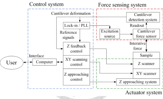
The force sensing system, actuator system, and control system are three main components of an AFM. A system block diagram is shown in Figure 2.1. The force sensing system measures the interative force between the cantilever tip and the sample.

For the dynamic mode, an excitation source is essential to resonate the cantilever. When the cantilever deformation is small, the cantilever force sensor is equivalent to a linear spring. The cantilever deformation is detected by the cantilever detection system, and is usually transduced to the voltage signal for the controller. The actuator system is responsible to produce the precise relative displacement between the tip and the sample.

The surface image is scanned through the XYZ scanner. Because the maximum displacement range of the scanner is usually at micrometer scale, the tip and the sample must be brought closely by another Z-axis approaching system. The control system recieves the cantilever deformation signal from the force sensing system, and commands the actuator system for the scanning. For the dynamic mode, a lock-in amplifier or a phase lock loop (PLL) is required for driving the excitation source and

(28)

approaching function, the Z-axis approaching system is also controlled by the control system. The user interface, data processes are executed by the software in the computer.

Furthermore, some additional implements can also be combined in the AFM system. An optical microscope (OM) and a XY coarse stage are helpful to specify the scanning area on the sample, when the sample has some larger features. The combination of the Raman spectroscopy and the fluorescence imaging can also be realized on the OM-based AFM for molecular identification.

Figure 2.1 Force sensing system, actuator system, and control system

2.2 Force Sensing System

2.2.1 Cantilever force sensor

The force sensor is a critical element in the AFM, and includes the cantilever and the tip. Figures 2.2 show the scanning electron microscope (SEM) images of commercial cantilever tips. The cantilever is based on a chip for handling easily. A tiny tip sites on the front end of the cantilever and faces to the measured sample. The structure is made by the microelectromechanical systems (MEMS) process. The

(29)

cantilever geometry is designed for different requirements. Figure 2.2(a) and Figure 2.2(b) present a rectangular cantilever and a triangular cantilever, respectively. The rectangular cantilever has uniform cross-section, and its spring constant and resonant frequency can be evaluated simply. The triangular cantilever is less sensitive to the lateral force and disturbance.

(a) Rectangular cantilever tip (b) Triangular cantilever tip Figure 2.2 SEM images of commercial cantilevers (MikroMasch)

The sharpness of the tip influences the resolution in XY plane directly. Nowadays, the apex radius of the commercial tip is about several nanometers. However, large force between the tip and the sample could wear the tip. The tip could also be polluted due to adherent dust or biomolecules. For example, a typical artifact caused by the double tips is illustrated in Figure 2.3(a). Two tips contact with the sample alternately, and cause an error on the scanning trajectory. Figure 2.3(b) shows the pectin aggregates image captured by the double tips [37].

(30)

(a) Scheme of double tips trajectory (b) Pectin aggregates image of double tips [37]

Figure 2.3 Double tips artifact

The cantilever is another significant component, which affects the force sensitivity and the scanning speed directly. When the cantilever deformation is much smaller than its dimensions, the cantilever can be seen as a linear spring. On a homogeneous rectangular cantilever, the spring constant k and the fundamental resonant frequency fr

of the fundamental flexural mode can be approximated by following Equations (2.1) and (2.2) [38]:

3 3

4L

k = Ebh , (2.1)

162 2

.

0 L

h f E

c

r ⁼ ρ , (2.2) where E is the Young’s modules of cantilever, b, h, and L are the width, thickness, and length of the cantilever, and ρc is the cantilever density.

For the contact mode, smaller spring constant k is preferred. Therefore, long and thin cantilevers are usually adapted. On the other hand, the dynamic mode often uses shorter and thicker cantilevers, which have higher resonant frequency fr. The cantilever with high resonant frequency can reduce the response time, and improve the scanning

(31)

speed. However, the spring constant is also increased. This result causes larger interactive force between the tip and the sample. To overcome this conflict, the cantilever size trends to diminish in all dimensions, including the length, width, and thickness. Besides, the cantilever detection system also needs to be modified for the smaller cantilever.

2.2.2 Excitation source

In the dynamic mode, the cantilever has to be excited around its resonant frequency.

The most common method utilizes a piezoelectric actuator to generate the oscillation energy as shown in Figure 2.4. The energy transfers to the cantilever through the mechanical parts on the cantilever holder. In liquid environment, “forest of peaks”

phenomenon also appears generally. For avoiding this problem, different methods such as magnetic excitation and photothermal excitation are also developed.

Figure 2.4 Scheme of piezoelectric actuator excitation

The magnetic excitation method applies an AC magnetic field on a magnetic cantilever as shown in Figure 2.5 [39, 40]. The magnetic excitation force applies on the cantilever directly, and a pure peak can be got in the tuning spectrum in liquid.

(32)

Figure 2.5 Scheme of magnetic excitation method [39]

The Lorentz force excitation method is illustrated in Figure 2.6 [41, 42]. Unlike the magnetic excitation method, the magnetic field is constant. The AC current passes through a triangular cantilever, and generates the vertical force on the cantilever.

However, this method could also induce a coupling between the flexural mode and the torsion mode of the cantilever [43]. Besides, it could affect the imaging due to the immersed electrode in liquid buffer.

Figure 2.6 Scheme of Lorentz force excitation method [42]

(33)

Figure 2.7 displays a setup of the photothermal excitation method [44, 45]. Except the cantilever detection system, an additional laser is focused on the cantilever. The cantilever oscillation is induced by the heat expansion, and the oscillation frequency is controlled through the laser modulation.

Figure 2.7 Scheme of photothermal excitation method

Summarizing these methods, applying excitation force on the cantilever directly is an effective way to eliminate the spurious peaks. However, additional equipment is required and complicates the system design. Furthermore, the magnetic and Lorentz force excitation methods limit the available cantilevers, and involve magnetic field and current into the measured environment. Therefore, some modifications based on piezoelectric excitation are also proposed on the other hand. Adams et al. studied the contact surface between the cantilever chip and the holder [46]. Typically in air, adjusting the cantilever position on the holder can eliminate the spurious peaks. Basing on this observation, the affection of dust or silicon shards on the cantilever is considered.

Through modifying the chip surface by adding pattern, lowering the chip contact surface area decreased the occurrence of spurious peaks. This result can likely be attributed to a higher occurrence of particles trapped on larger contact area.

(34)

Figure 2.8 Cantilever holder design of Asakawa and Fukuma [47]

Asakawa and Fukuma considered the acoustic wave propagation from the piezoelectric actuator to the cantilever, and proposed a holder structure as shown in Figure 2.8 [47]. First, for suppressing the acoustic wave caused by the holder boundary stress, a PEEK holder body was placed between the piezoelectric actuator and the steel chip support. Second, the cantilever was excited by the flexure drive mechanism, which was achieved by a flexure hinge design as shown in Figure 2.8(c). Figure 2.9 shows the experimental results of their modified holder with two different holder materials. Figure 2.9(a) represents the bode plot with the steel holder body, and Figure 2.9(b) is the bode plot with the PEEK material. A single peak was captured on the PEEK holder successfully. However, the flexure drive mechanism caused the phase delay, which may need to be compensated for the FM-AFM and phase imaging.

(35)

(a) Bode plot on steel holder (b) Bode plot on PEEK holder Figure 2.9 Excitation spectrum comparison between two materials [47]

2.2.3 Cantilever detection system

The deformation of the cantilever has to be detected by a detection system. The resolution of the detection system affects the AFM force sensitivity directly. Besides, the bandwidth of the cantilever detection system also limits the scanning speed. Several detection methods are shown in Figure 2.10. The earliest method utilizes a STM tip to measure the tunneling current between the STM tip and the cantilever as shown in Figure 2.10(a) [4]. Utilizing the resistance variation of a piezoresistive cantilever, the cantilever deflection can be measured by a Wheatstone bridge as shown in Figure 2.10(b) [48]. This embedded piezoresistive sensor on the cantilever simplifies the alignment of the external detection sensor, but also complicates the cantilever

(36)

(a) Tunneling current (b) Piezoresistance (c) Capacitance

(d) Interference (e) Beam deflection (f) Astigmatism Figure 2.10 Cantilever detection methods

environment. Besides the electric methods, different optical methods are also utilized.

Figure 2.10(d) shows the interferometry method using an optical fiber, and this method has high sensitivity and provides absolute displacement measurement [50]. This technique needs the complex signal processing and implementation cost, and positioning the optical fiber is also a demanding task. The optical beam deflection method is the most popular method, and its principle is illustrated in Figure 2.10(e) [51, 52]. In this method, a laser beam is focused on the cantilever, and the reflective beam is detected by a position sensing detector (PSD). Beam deflection method is sensitive to the cantilever angular variation, and provides both the cantilever flexural and torsional deflection signals. The astigmatic detection method is widely used in the digital versatile disk (DVD) pickup head. Figure 2.10(f) is a schematic setup for the cantilever detection [53, 54]. The vertical displacement and two-dimensional angular tilts of the cantilever can be detected in this method. Utilizing the commercial astigmatic pickup

(37)

head, an astigmatic detection system can be compact and cheap. Furthermore, it has small laser spot size and high bandwidth. The detailed comparison between beam deflection and astigmatic detection methods is discussed in Chapter 5.

2.3 Actuator System

2.3.1 Scanner

The AFM scanner provides precise relative displacement between the cantilever tip and the sample. By moving either the tip or the sample, the AFM design can be classified to the scanning tip type or the scanning sample type roughly. For applications with small and light samples, the scanning sample type is prefered, because its bandwidth doesn’t reduces much due to the weight of sample. On the other hand, the scanning tip type is suitable for the large and heavy sample. However, the affection on the cantilever detection system due to the movement has to be avoided.

Most AFM scanners use the piezoelectric material to achieve precise displacement.

Piezoelectric ceramic material such as lead zirconate titanate (PZT) is a transducer between the electric charge and the mechanical force. The piezoelectric actuator can produce extension through applying voltage directly, and generates precise displacement.

On the contrary, high input voltage is required for larger displacement. The multilayer piezoelectric stack increases the displacement by stacking piezoelectric actuators as shown in Figure 2.11(a). A three-axes scanner can be achieved by collocating three piezoelectric stacks with an appropriate mechanism. The piezoelectric tube is another common design for the AFM scanner. The piezoelectric tube has upper and lower sections as shown in Figure 2.11(b). The outside electrode of the upper section is

(38)

electrodes provides one dimensional movement. Therefore, the upper section is responsible for the XY-axes movement, and the lower section controls the Z-axis extension. The tube scanner can provide the three-axes movement by one single structure, and simplifies the assembling problem. However, the XY-axes movement causes crosstalk on the Z-axis when the scanning area is far from the tube center.

Another drawback of the tube scanner is the spacial limitation. The tube scanner occupies the bottom space of the sample, and the invert OM is not compatible.

(a) Multilayer piezoelectric stack (b) Piezoelectric tube Figure 2.11 Piezoelectric scanner

Although the piezoelectric actuator is precise and easy to use, nonlinear and changeable properties of the piezoelectric actuator should be reminded. Similar to the electromagnetic actuator, the hysteresis phenomenon also exhibits on the piezoelectric actuator. In the piezoelectric material, hysteresis is caused by crystalline polarization effects and the molecular friction. Figure 2.12 illustrates the hysteresis phenomenon, where the X-axis and Y-axis are the input voltage and output displacement respectively.

(39)

The hysteresis effect is related to operation parameters such as input amplitude, load, temperature, etc. This nonlinear property causes the image distortion problem as shown in Figure 2.13(a). The sample is a square grating with 3 μm pitch and 20 nm height. The distortion of the square structures is obvious due to the hysteresis. Another issue is the scanner bandwidth, which limits the maximum scanning speed. Without the Z-axis feedback control, Figure 2.13(b) shows the cantilever deflection image of the same square grating with 800 line/sec scanning rate. Because the Z displacement of the scanner is constant, the deflection signal is proportional to the topography. The high scanning rate causes serious distortion and oscillation, and the scanning range also decreases. Except the scanner properties, the environmental temperature variation can induce a slow position drift due to the thermal expansion of the whole mechanism.

Figure 2.12 Piezoelectric hysteresis with different input amplitudes

(40)

(a) Topography image with scanning rate of 1 line/sec

(b) Deflection image with scanning rate of 800 line/sec Figure 2.13 AFM images of calibration grating with 3 μm pitch

Some nonlinear scanner properties can be solved by control methods. The open-loop control method calibrates the scanner displacement by adjusting the input driving signal. The upper diagram of Figure 2.14 is a typical calibrated driving waveform, and the output displacement becomes linear as the lower diagram. The open-loop calibration can solve the hysteresis phenomenon, but can’t deal with the thermal drift problem.

(41)

Figure 2.14 Open-loop scanner calibration

The closed-loop method performs an accurate positioning by a feedback control loop as shown in Figure 2.15(a). In this method, a position sensor detects the accurate displacement of the actuator. Then, the actuator displacement signal is compared with the target signal, and a controller compensates the driving signal to minimize the error signal. The proportional-integral-derivation (PID) controller is used in the AFM generally. For optimizing the performance, the PID gains should be adjusted for applications. Figure 2.15(b) demonstrates the step response with different controller gains setting. If the gains are too high, the overshooting occurs and causes an oscillation.

On the contrast, the settling time will be extended when the gains are reduced. The closed-loop is helpful for the applications that need accurate positioning. However, the essential position sensor also complicates the scanner design, and the sensor noise restricts the scanning resolution.

(42)

(a) System block diagram

(b) Step response with different controller gains Figure 2.15 Closed-loop scanner control

2.3.2 Z-axis approaching system

Before scanning, the cantilever tip must approach the sample surface into the scanner range. This step can be achieved by manual operation or a motorized system.

The stepper motor system is easy to control the displacement, and is widely used for approaching. Two considerations here are the tip colliding and time consumption, and two tactics are introduced as follows.

In the continuous approaching method, the Z-axis scanner and the stepper motor work simultaneously. The Z-axis feedback controller monitors the tip-sample interactive force during the stepper motor running. When the tip contacts with the sample, the scanner will draw back. After the scanner retracting to its half range, the stepper motor stops. In this method, the motor speed and feedback parameters must be adjusted

(43)

appropriately. Otherwise, the impact force could damage the tip at the contact instant.

In the alternate approaching method, the Z-axis scanner and the stepper motor work alternately. After the stepper motor running a small distance, the force-displacement curve is performed to detect the tip-sample distance. Similarly, this loop stops when the sample is located around the half range of the scanner. The alternate approaching method can avoid large interactive force during approaching. However, it cost more time than the continuous approaching method. For improving the approaching efficiency, an OM can monitor the tip-sample distance roughly. First, the tip is brought close to the sample rapidly with the OM monitor. Then, the alternate approaching method is adopted.

2.4 Control System

Various functions such as the scanning and the force-displacement curve measurement are controlled by the control system. The digital control system is flexible for adjusting parameters, and is adopted in most AFM systems. In the tapping mode AFM, the lock-in amplifier is necessary for getting the cantilever amplitude and phase signals. The Z-axis feedback control collaborates with the XY-axes scanning function for measuring the surface image.

2.4.1 Lock-in amplifier

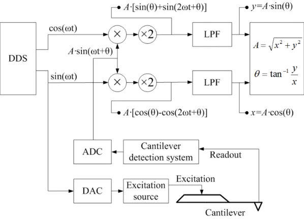
Figure 2.16 illustrates the principle of a digital lock-in amplifier. The sinusoidal driving signal with frequency ω is generated by a direct digital synthesizer (DDS), and transferred to the excitation source after a digital-to-analog converter (DAC). For simplification, the supposed cantilever response is an ideal sinusoidal wave with

(44)

multiplied by sin(ωt) and cos(ωt), respectively. After a low pass filter (LPF), the remaining dc terms x and y represent the Cartesian coordinates of the point on the unit circle. Therefore, A and θ can be calculated by trigonometric functions. In practice, these signal processing can be realized by the field-programmable gate array (FPGA) or the digital signal processor (DSP). During scanning, the cantilever response could not be an ideal sinusoidal wave due to the complex interactive force with the sample.

Lowering the cutoff frequency of LPF can reduce the noise, but the bandwidth is also reduced.

Figure 2.16 Digital lock-in amplifier diagram

2.4.2 Z-axis feedback control

The Z-axis feedback controller is responsible for adjusting the interactive force between the tip and the sample. Figure 2.17 presents a Z-axis feedback loop. At first, user determines the setpoint, which is the tracking value of the reference signal. The

(45)

reference signal depends on the operation mode. In the contact mode, the cantilever deflection signal is selected for reference. In the dynamic mode, the amplitude, the phase, or the frequency signal can be adopted. The error between the setpoint and the reference signal is inputted to a PID controller, and the driving signal to the Z-axis scanner is generated. The Z-axis displacement of the scanner is adjusted to minimize the error signal. During the scanning, the tip-sample distance can be kept constant, and the Z-axis displacement represents the topography of the sample. Similar to the closed-loop scanner control, the PID gains should be adjusted to optimize the tracking performance.

However, this adjustment is much difficult in the Z-axis feedback control than the closed-loop scanner control. In the closed-loop scanner, only the sample weight changes.

On the other hand, the tip and sample system is complicated. Various interactive forces such as the mechanical contact force, van der Waals force, electrostatic force and capillary force exist between the tip and the sample. Besides, the tip geometry, environmental humidity, pressure, temperature and sample material also affect these interactive forces. Therefore, the scanning parameters are adjusted according to the scanning conditions.

Figure 2.17 Z-axis feedback control diagram

(46)

2.4.3 XY-axes scanning control

The XY-axes scanning control is used for measuring an area data. The raster scan is the most common method, and Figure 2.18(a) shows its trajectory on the XY plane. In this case, X-axis is the fast axis, which moves forward and backward. Then the slow Y-axis moves to the next line. A square area can be scanned after repeating these two steps. This method is intuitional and easy to program. The surface information can be presented in a two dimensional array, which is easy for the image process and display.

However, the triangular waveform of the fast axis contains harmonic terms with higher frequencies. It is unfavorable for the high speed scanning, and could induce oscillations easily.

Another method called the spiral scan method is proposed for high speed applications [55]. The cosine and sine signals with varying amplitudes are applied to X-axis and Y-axis, and produce a spiral trajectory as shown in Figure 2.18(b). The spiral trajectory without suddenly direction change is more suitable for the high speed scanning. However, the image process and the pixel mapping on the monitor become more complicated.

(a) Raster scan (b) Spiral scan Figure 2.18 XY-axes scanning control

(47)

Chapter 3 Cantilever Force Sensor

The cantilever tip is a sensitive force sensor in the AFM, and its dynamic properties in liquid are significant for scanning speed and quality. In this chapter, the dimensional effect and high order resonances of the cantilever are discussed theoretically and experimentally.

3.1 Cantilever Dimensional Effect

3.1.1 Theoretical calculation

The rectangular cantilever has a uniform cross-section and is the most common geometric design for the AFM. The governing equation of the cantilever deflection is derived under several assumptions as follows: (1) The cross-section is uniform; (2) The cantileve length is greatly larger than its width; (3) The cantilever is isotropic, linear, and elastic matercial; (4) The cantilever deflection is far smaller than the cantilever dimensions. According to the Euler–Lagrange equation [56], the dynamic deflection of the cantilever is expressed as Equation (3.1)

) , ) (

, ( )

, (

2 2 4

4

t x t f

t x bh w x

t x

EI w _c =

∂ + ∂

∂

∂ ρ , (3.1)

where E is the Young’s modules of the cantilever, I is the moment of inertial of the cantilever, ρc is the cantilever density, b and h are the width and the thickness of the cantilever, x is the spatial coordinate along the cantilever length, t is time, w(x,t) is the cantilever flexural deflection, and f(x,t) is the external applied force per unit length.

Utilizing the separation of variables, w(x,t) is separated into the time and spacial

(48)

where W(x) is the shape function, and T(t) is the time-dependent function. Considering the case of an undamping free vibration without the external force f(x,t), Equation (3.3) is obtained by substituting Equation (3.2) into Equation (3.1):

) 0 ( ) ( 1 ) ( )

( ²

2 4

4

=

+ dt

t T d t dx T

x W d x bhW

EI

ρc . (3.3)

The solution of T(t) must be periodic. Assuming the radial resonant frequency of the cantilever in vacuum is ωvac, W(x) and T(t) can be solved by

2 2

2 4

4 ( )

) ( 1 )

( )

( ^vac

c dt

t T d t T dx

x W d x bhW

EI ω

ρ ⁼⁻ ⁼ . (3.4)

Substituting the boundary conditions at the clamped fix end and the free end, the shape function is obtained:

) cosh )(cos

cosh cos

sinh (sin

sinh sin

)

( x

L x C

L C C

C

C x C

L x C

W ⁿ ⁿ

n n

n

n −

+

− +

−

= , (3.5)

where

vac c

n L

EI

C2 = ρ bh 2ω , (3.6)

which satisfies the equation

0 cosh cos

1+ Cn Cn = . (3.7) Equation (3.7) has infinite solutions Cn. Therefore, infinite shape functions W(x) exist, and represent different order resonances. The corresponded resonant frequency of the nth order resonance in vacuum is given by

c n

c n n vac

E L h C bh EI L

C

ρ ω , ₂² ρ ² ₂

= 12

= . (3.8)

where L is the length of the cantilever. For an incompressible fluid environment, Sader introduced a hydrodynamic load into Equation (3.1) [57]. Through the Fourier transform of Equation (3.1), the dynamic equation becomes

(49)

) , ( ) , ) (

,

( 2

4 4

ω ω

ω

ω ρ _bh _W _x _F _x

dx x W

EI d − _c = , (3.9)

where ω represents the vibrational frequency, and the external force is distinguished into two contributions:

^F(^x,ω)= ^Fhydro(^x,ω)+^Fdrive(^x,ω), (3.10) where Fhydro(x,ω) and Fdrive(x,ω) are the hydrodynamic load and the drive force, respectively. Based on the equations of motion for fluid, the general form of Fhydro(x,ω) is given by

( ,Re) ( , ) ) 4

,

(^x ω π ρ ω²^b² κ ^W ^x ω

F_hydro = _f Γ , (3.11)

where ρf is the fluid density, and Γ(κ,Re) is the dimensionless hydrodynamic function, which depends on the Reynolds number Re and the aspect ratio κ:

μ ρω ²

Re b

= , (3.12)

L C_n b

κ = , (3.13)

where μ is the viscosity of the fluid. According to the Navier-Stokes equation, Γ(κ,Re) is given by [58,59]

8 1

Re) ,

( = a

Γ κ , (3.14) where the coefficient a1 is solved by the linear equations



= 

>

= =

M +

m

m m q m

q q

a q A A

1

Re ,

, 0, 1

1 , ) 1

( ^κ , (3.15)

where the integer M must be large enough to obtain a convergent solution, and A^κq,m and A^Req,m are the terms of Meijer G functions:

(50)









−

− +

− −

= ⁻

m q m q G i

A

q m

q 0 2

2 / 1 16

Re

2 21 ²

13 5 4 2

, κ

κ π

κ









+

−

− +

− ⁻ −

1 1

0

2 / 1 16

Re

2 21 ²

13 1 4

m q m q G i

q κ

π . (3.17)

Substituting Equations (3.10) and (3.11) into Equation (3.9), the dynamic equation becomes

EI x x F

h W b EI

bh dx

x W

d _drive

c

c f ( , )

) , ( Re) , 4 (

) 1 ,

( ²

4

4 κ ω ω

ρ ω πρ

ρ

ω ₌



 



 + Γ

− . (3.18)

For calculating the resonant frequency in fluid, Fdrive(x,ω) is neglected, and Equation (3.8) is substituted into Equation (3.18) to obtain

0 ) , ( Re) , 4 (

) 1 , (

2 , 4

2 4 4

4

 =



 



 + Γ

− κ ω

ρ πρ ω

ω ω _W _x

h b L

C dx

x W d

c f n

vac

n . (3.19)

Neglecting dissipative effects, the relation between the resonant frequencies in fluid ωfluid and vacuum ωvac is described by

2 / 1

Re) , 4 (

1

−



 



 + Γ

= κ

ρ πρ ω

ω

r c f vac

fluid

h

b , (3.20)

and the Q-factor is

Re) , (

Re) , ( ) / 4 (

κ

κ πρ

ρ

i

r f

ch b

Q Γ

Γ

= + , (3.21)

where the subscript r and i refer to the real and imaginary components of Γ(κ,Re). For numerical calculation of a silicon cantilever in water, the values of the parameters are listed in Table 3.1. For calculating Re initially, the frequency in Equation (3.12) is evaluated by

2 / 1

, 1 4

−



 



 +

= h

b

c f n

vac ρ

ω πρ

ω . (3.22)

(51)

Table 3.1 Numerical values of parameters

Symbol Description Value

E Young’s modules of cantilever 169 × 10^-9 N/m² C1 Dimensionless number of first resonance 1.8751

ρc Cantilever density 2330 kg/m³

L Length of cantilever 30 ~ 300 μm

b Width of cantilever 5 ~ 50 μm

h Thickness of cantilever 0.25 ~ 1 μm

I Moment of inertial of cantilever b·h³/12 k Spring constant of cantilever Ebh³/4L³

μ Viscosity of water 8.94 × 10^-4 Pa·s (at 25 ^oC)

ρf Density of water 997 kg/m³(at 25 ^oC)

M Number of summation in Equation (3.15) 10

The resonant frequency fr in hertz, the Q-factor Q, and the spring constant k of the cantilever are calculated under different cantilever length L, width b, and thickness h.

Figures 3.1(a), (b), and (c) present the cantilever properties with the cantilever thicknesses h of 0.25 μm, 0.5 μm, and 1 μm, respectively. The longer cantilever has smaller k, but lower fr and Q. Broadening the cantilever width can increase the Q, but reduces fr and raises k. The thicker cantilever not only increases fr and Q, but also raises k. Therefore, fr, Q, and k can’t be improved simultaneously through modifying any single dimension of the cantilever directly.

(52)

(a) h = 0.25 μm (b) h = 0.5 μm (c) h = 0.1 μm Figure 3.1 Cantilever properties versus cantilever dimensions

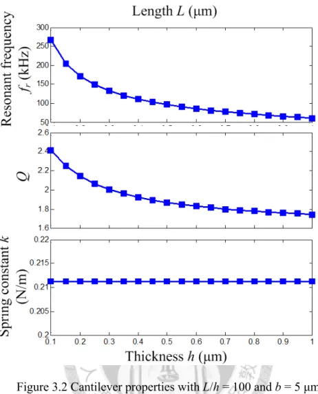
According to Equation (2.1), the spring constant k is dominated by the cantilever length L and thickness h. Therefore, k can be kept constant through fixing the L to h ratio and the width b. Figure 3.2 shows the cantilever properties with L/h = 100 and b = 5 μm. The result shows that the resonant frequency fr and the Q-factor can be increased through decreasing h and L proportionally.

(53)

Figure 3.2 Cantilever properties with L/h = 100 and b = 5 μm

3.1.2 Experimental results

For examining the cantilever dimensional effects, the width and the length of cantilevers are modified. The manufacturing process is performed in a dual beam focused ion beam (FIB) system (NOVA-600, FEI). The cantilever material is removed through Gallium ions collision in a vacuum condition. For eliminating the individual difference between cantilevers, the measurement and modification are repeated on an identical cantilever. Figure 3.3 shows a commercial cantilever (PPP-NCHAuD, NANOSENSORS), which is modifed from the widths of 37 μm to 14 μm. The

(54)

cantilever length (138 μm) and thickness (4 μm) are measured by SEM. The cantilever has an Au coating on the detector side of the cantilever for increasing the reflectivity.

(a) b = 37 μm (b) b = 31 μm (c) b = 24 μm

(d) b = 17 μm (e) b = 14 μm Figure 3.3 Cantilever No.02 with different widths

For measuring the resonant frequency and the Q-factor in air and water, a commercial AFM (MultiMode, Bruker) is utilized. Without external excitation, the thermal fluctuation spectrum is acquired through the fast Fourier transform (FFT) of the cantilever deflection signal. The resonant frequency fr,wm with width-modification and thr Q-factor are calculated from the fitting curve of the thermal fluctuation spectrum.

The sum voltage Usum of the PSD represents the laser intensity on the PSD. Two cantilevers (cantilever No.01 and No.02) are measured in the same process, and the results are listed in Table 3.2.