以淤泥實驗探討壓密、射流、擾動及水力抽砂行為之研究

(1)

國立臺灣大學工學院土木工程學系碩士論文

Department of Civil Engineering College of Engineering National Taiwan University

Master Thesis

以淤泥實驗探討壓密、射流、擾動及水力抽砂行為之研究 Consolidation, jetting, stirring and hydrosuction of

experimental mud deposits

葉亭霞 Ting-Sia Ye

指導教授：卡艾瑋教授 Advisor: Dr. Hervé Capart

中華民國 105 年 7 月

July, 2016

(2)

誌謝

轉眼研究所兩年即將畫下句點。I deeply appreciate my advisor, Hervé Capart.

You always encourage us to try and give us useful advice on research. I really admire your attitude toward research. 也謝謝周憲德老師、吳富春老師和賴悅仁老師，撥冗擔任我的口試委員，給予我的論文建議與指導，讓論文能夠更加完整。

謝謝大地組的葛宇甯老師，多次向您請教有關土壤力學實驗和觀念上的問題，

謝謝您總是很親切地為我解惑；謝謝工科海的連師傅，幫忙製作實驗需要的裝置，

也透過自身豐富的經驗，給予我實驗許多建議；謝謝土力實驗室的郭銘雄技士，

指導我操作動三軸試驗儀，細心地提醒我必須注意的細節和流程；謝謝老大、韜哥和啟耀學長，從你們身上學到許多卡門需要具備的能力，你們總是非常有耐心為我們解答疑惑、陪著我們解決實驗上的困難，老師不在台灣的這一年，扮演兄長如父的角色，讓我們非常安心；謝謝阿宜、志中兩位卡門戰友，一起修課、打掃研究室、出野外測量，共享卡門甘苦，互相幫忙、鼓勵和崩潰；謝謝蔡門三兄弟、富建、品慶，你們總是義不容辭在我實驗需要人手的時候給予協助以及各種大小事的幫忙；謝謝鈺倢陪我分享生活的大小事，為有時苦悶的研究生活增加樂趣；很開心研究所認識這一群朋友，除了在研究和課業上互相切磋學習，也一起吃飯聊天出遊，讓研究所生活更加多彩有趣，創造了許多很棒的回憶；謝謝室友真誼，從國中認識到現在，研究所有幸一起同住，讓我在台北也感受到如同家人般的關心和陪伴；謝謝璟瑜和家宜，幫忙我們處理很多研究室的公務，實驗上也謝謝妳們的協助，讓我們可以沒有後顧之憂全力衝刺論文；謝謝建霖的照顧和陪伴，有時忍受我的脾氣和任性，感性的話就不寫在這兒了我會害羞；最後，謝謝我最親愛的爸爸媽媽和兩位哥哥，你們全力的支持和無條件的付出，讓我總是可以無憂地當你們的小公主，能夠和你們成為家人，是我最幸福的事。

(3)

中文摘要

本研究目的在於探討不同自重壓密天數下的土壤特性及外力裝置對水力抽砂的影響，試圖找出最佳效率的抽泥方法。論文分成兩部分:第一部分為了解土壤特性，透過在不同壓密天數下，記錄淤泥表面得到每日壓密量、以 T 型貫入實驗得到剪力強度和取樣方式得到分層密度，並建立壓密理論與實驗結果進行比較；第二部分為水力抽砂實驗，過去研究顯示，水力抽砂在長天數的條件下，因為土體強度太大，效果有限，因此本論文著重於此，設計在不同壓密天數的條件下，分別配置水刀、絞刀破壞土壤結構，同時進行水力抽砂，此外，配合雷射掃描方式記錄抽泥前後的地形，結果顯示，在無外力裝置的情形下，抽砂效率會隨著天數增加而降低，然而，對於短天數而言，有無搭配外力並沒有明顯差別，但對於長天數來說，外力裝置確實發揮功用，使得水力抽砂順利進行，效果較無外力裝置大幅提升。

關鍵字：水力抽砂、自重壓密、水刀、絞刀、土壤特性

(4)

ABSTRACT

In order to alleviate problems caused by reservoir sedimentation, the hydrosuction is an effective way for deposition removal. To help interpret the sediment properties of different self-weight consolidation duration, we investigated the shear strength by T-bar testing, density by sampling and settlement by record. Besides, the consolidation theory is built to compare with experiment results. Moreover, compared to previous research, we conducted a series of hydrosuction experiments focused on long consolidation duration, in which hydrosuction had limitation in withdrawal. In addition to the reduced-scale hydrosuction, water jet or rotary cutter was equipped as an external force to damage sediment structure by jetting and stirring. The result shows that the efficiency of hydrosuction with no equipment gets worse as consolidation duration increases.

Furthermore, the external force equipment works well in long consolidation duration yet not sufficiently in short.

Keywords: hydrosuction; self-weight consolidation; water jet; rotary cutter; soil property

(5)

LIST OF FIGURES

Fig. 1.1 Photo of the mobile barge with hydrosuction in Shihmen Reservoir, northern

Taiwan ... 1

Fig. 1.2 External force equipment in Shihmen Reservoir: (A) water jet (B) rotary cutter 3 Fig. 2.1 Sketch of excess pore water pressure conditions ... 11

Fig. 2.2 Settlement evolution of different elevation ... 13

Fig. 2.3 Shear strength comparison for different consolidation duration ... 13

Fig. 2.4 Layer density comparison for different consolidation duration ... 14

Fig. 3.1 Tank: (A) sketch and size (B) photo ... 18

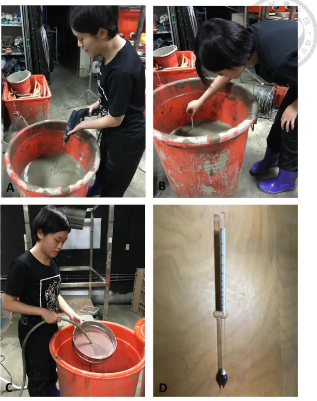
Fig. 3.2 Sediment sample preparation procedure: (A) mixing (B) measuring (C) filtering (D) hydrometer... 19

Fig. 3.3 The mark of record ... 20

Fig. 3.4 Relation between consolidation duration and elevation ... 21

Fig. 3.5 Relation between consolidation duration and degree of consolidation ... 21

Fig. 3.6 Soil triaxial tester ... 23

Fig. 3.7 T-bar: (A) photo (B) connection (C) sketch and size ... 24

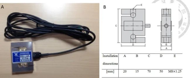
Fig. 3.8 S load cell: (A) photo (B) sketch and size ... 25

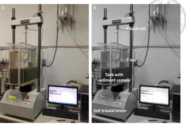
Fig. 3.9 Setup of shear strength experiment: (A) photo (B) interpretation ... 26

Fig. 3.10 Procedure of shear strength experiment: (A) stand the sediment sample for consolidation duration. (B) let lifting platform go upward. (C) A close look when T-bar is pushed in the sediment sample. ... 27

Fig. 3.11 Calibration: (A) compression (B) tension ... 28

Fig. 3.12 Three types of buoyance calculation for 1 day ... 32

(9)

Fig. 3.13 Three types of buoyance calculation for 3 days ... 32

Fig. 3.17 Shear strength for 1 day ... 35

Fig. 3.18 Shear strength for 3 days ... 35

Fig. 3.22 Comparison of Shear strength for different consolidation duration ... 37

Fig. 3.23 Sketch of acrylic Layer ... 38

Fig. 3.24 Tank with acrylic layers: (A) sketch and size (B) photo ... 39

Fig. 3.25 Standing the tanks for expected consolidation duration... 39

Fig. 3.26 Layer density experimental procedure: (A) acrylic layer removal (B) empty sampling bottles (C) sampling bottles with sediment (D) weighing (E) aluminum bowls with sediment (F) drying ... 41

Fig. 3.27 Layer density profile for 1 day ... 42

Fig. 3.28 Layer density profile for 3 days ... 42

Fig. 3.32 Time evolution of the density profile ... 44

Fig. 4.1 Settlement comparison ... 48

Fig. 4.2 Shear strength comparison for 1 day ... 49

Fig. 4.3 Shear strength comparison for 3 days ... 49

(10)

Fig. 4.7 Shear strength comparison of theory with experiment for all duration ... 51

Fig. 4.8 Layer density comparison for 1 day ... 52

Fig. 4.9 Layer density comparison for 3 days ... 52

Fig. 4.13 Layer density comparison of theory with experiment for all duration ... 54

Fig. 4.14 Theory and experiment comparison of the relation between shear strength and void ratio ... 55

Fig. 4.15 Theory and experiment comparison of the relation between shear strength and void ratio from 1 to 5 ... 56

Fig. 4.16 Theory and experiment comparison of the relation between log shear strength and void ratio from 1 to 5 ... 56

Fig. 4.17 Settlement comparison after delaying consolidation duration ... 57

Fig. 4.18 Shear strength comparison after delaying consolidation duration ... 58

Fig. 4.19 Layer density comparison after delaying consolidation duration ... 58

Fig. 5.1 Conceptual sketch of experimental setup ... 64

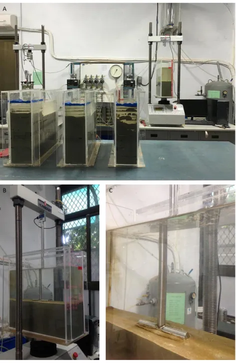
Fig. 5.2 Photo of experimental setup ... 64

Fig. 5.3 Tank ... 65

Fig. 5.4 Open for overflow ... 65

Fig. 5.5 Constant head water supply tank ... 66

Fig. 5.6 Energy dissipation box ... 66

(11)

Fig. 5.7 Hydrosuction pipe ... 67

Fig. 5.8 Vacuum pump ... 67

Fig. 5.9 Vertical screw ... 68

Fig. 5.10 Horizontal linear slide ... 69

Fig. 5.11 (A) Densimeter (B) Datalog ... 69

Fig. 5.12 Hydrosuction with external force equipment in Shihmen Reservoir: (A) water jet (B) rotary cutter ... 70

Fig. 5.13 Laboratory water jet ... 71

Fig. 5.14 High pressure water pump ... 71

Fig. 5.15 Arrangement of water jet ... 72

Fig. 5.16 Laboratory rotary cutter ... 73

Fig. 5.17 Arrangement of rotary cutter ... 74

Fig. 5.18 Experiment frame, tank and cart ... 75

Fig. 6.1 (A) Laser light (B) Thickness of laser sheet ... 80

Fig. 6.2 Laser mobile track ... 80

Fig. 6.3 Laser holder and platform ... 81

Fig. 6.4 Frame ... 81

Fig. 6.5 Photo of JVC GC-PX100 ... 82

Fig. 6.6 Camcorder arrangement ... 83

Fig. 6.7 Calibration target: (A) sketch and size (B) photo ... 84

Fig. 6.8 Calibration target is placed in the tank with the origin. ... 84

Fig. 6.9 Calibrations ... 85

Fig. 6.10 Image pre-processing: (A) before (B) after ... 86

Fig. 6.11 Transferred 3D lines ... 87

Fig. 6.12 Digital terrain model ... 88

(12)

Fig. 7.1 Comparison of mass conservation of hollow ... 92

Fig. 7.2 Density comparison with no equipment ... 94

Fig. 7.3 DTM comparison with no equipment: (A) 3 days (B) 7 days (C) 14 days ... 95

Fig. 7.4 Density comparison with water jet ... 96

Fig. 7.5 DTM comparison with water jet: (A) 3 days (B) 7 days (C) 14 days (D) 30 days97 Fig. 7.6 Density comparison with rotary cutter ... 98

Fig. 7.7 DTM comparison with rotary cutter: (A) 3 days (B) 7 days (C) 14 days (D) 30 days ... 99

Fig. 7.8 Density comparison for 3 days ... 100

Fig. 7.9 DTM comparison for 3 days: (A) no equipment (B) water jet (C) rotary cutter101 Fig. 7.10 Density comparison for 7 days ... 102

Fig. 7.15 DTM comparison for 30 days: (A) water jet (B) rotary cutter ... 107

(13)

LIST OF TABLES

Table 2-1 Mass conservation of layer density ... 15

Table 3-1 Sediment properties ... 18

Table 3-2 Specification of S load cell ... 25

Table 6-1 Specification of JVC GC-PX100 ... 82

Table 7-1 List of hydrosuction experiment cases ... 89

Table 7-2 Result of mass conservation of hollow ... 92

(14)

Chapter 1 Introduction

Fig. 1.1 Photo of the mobile barge with hydrosuction in Shihmen Reservoir, northern Taiwan

Deposition of fine sediment near the dam in reservoirs causes some problems in not only Taiwan but also many other countries (Fan and Morris, 1992; Schleiss et al., 2010). The sediment accumulation may clog the water supply and power generator intakes in short term while reducing the capacity of reservoir in long term. To address

(15)

operation processes are withdrawing slurry in the bottom of reservoir by pumping or siphoning, then carrying downstream to settling ponds via floating pipeline (Hotchkiss and Huang, 1995). Moreover, the hydrosuction is equipped on the mobile barge which allows it to move to the area of concern (Fig. 1.1).

Previous research states that the concentration of sediment withdrawal is related to the sediment consolidation duration (Ke et al., 2016). Besides, experiments show that when the consolidation duration exceeds 14 days, the hydrosuction has limitation in withdrawal because of the high degree of consolidation (Chen, 2015). In other words, the longer the duration is, the less the hydrosuction efficiency is. The phenomenon is also found in sediment removal of hydrosuction in field site. On account of the fact, water jet and rotary cutter serve as external force to damage the structure of sediment;

therefore, the hydrosuction can withdraw slurry in high efficiency (Fig. 1.2).

On the other hand, the soil properties of different consolidation duration are of interest. Through comprehending the soil characteristic of a certain consolidation duration even a certain elevation, the hydrosuction can be adjusted to withdraw the slurry according to its property. To put it differently, the soil properties can be applied to promote the efficiency of withdrawal.

Therefore, the thesis focuses on the long consolidation duration cases and soil properties which are different form previous research. It is divided into two parts: (i) consolidation, and (ii) hydrosuction.

In first part, the objective is to understand the physical mechanism of consolidation process. The consolidation theory is developed to obtain the theoretical soil properties, e.g. settlement, shear strength, and layer density (Chapter 2). Besides, the three experiments are separately conducted to yield experimental results (Chapter 3). Then, the comparison of theory with experiment would be demonstrated in Chapter 4.

(16)

In second part, the hydrosuction experiments are carried out to simulate the behavior of withdrawal of different consolidation duration and two kinds of external force, jetting by water jet and stirring by rotary cutter, in order to find out the most efficient fashion. The experimental material, setup and procedure are addressed in Chapter 5. Chapter 6 illustrates the image processing of laser scan to get the DTM. Last, the results and comparison are presented in Chapter 7.

Fig. 1.2 External force equipment in Shihmen Reservoir: (A) water jet (B) rotary cutter

(17)

(18)

(19)

(20)

Chapter 2 Theory

Equation Chapter 2 Section 1

2.1 Framework of Theory

In this theory, Lagrangian coordinate system is used to describe the position throughout the consolidation process. The element is labeled according to its initial position, which is independent of time, in Lagrangian coordinate system. The detail description of Lagrangian coordinate system used in consolidation is addressed in Lin (1983).

Let Z_s( , t) be the position at time t of the sediment material plane located at elevation Z_s  . If the rigid floor of the tank is at elevation z0 , we have the initial and boundary conditions

( , 0)

Zs   (2.1)

(0, ) 0

Zs t  (2.2)

The downward speed of sediment grains (W_s) is accordingly

s s

W Z t

 

 (2.3)

Let c_s( , ) t be the volumetric concentration of the sediment grains of material plan  at time t. The corresponding mass density ( ) per unit volume of space

(21)

(void + grains) is

( , )t _Sc_s _W(1 c_s)

     (2.4)

where _S is the density of dry solid; _W is the density of water.

Using these variables, conservation of sediment mass can be expressed as ( , ) ^s( , ) ( , 0)

s s

c  t z  t c 



 

 (2.5)

Moreover, according to soil mechanics, total stress ( ) is ' u_w

   (2.6)

where ' is effective stress; u_w is total water pressure.

Besides, total water pressure (u_w) can be divided into two parts

w ss e

u u u (2.7)

where u_ss is static water pressure; u_e is excess pore water pressure.

Thus, total stress can be expressed as

' (u_ss u_e)

    (2.8)

In addition, total stress can be calculated by

m( ) d

d

  

 ^{ } (2.9)

where _m is moist unit weight.

In the same way, static water pressure also can be calculated by

ss ( )

w

du

d  

 ^{ } (2.10)

where _w is water unit weight.

Based on Terzaghi’s theory of one-dimensional consolidation, we have the governing equation to solve the excess pore water pressure

(22)

2 2

e e

v

u u

c  t

 

  (2.11)

where c_v is coefficient of consolidation.

Boundary conditions and initial condition are as follow

0

(0, )

0, ( , ) 0

e

u t

u h t



  

 (2.12)

 

^,0

 

e ss m w

u    u      (2.13)

However, Terzaghi’s theory of one-dimensional consolidation is suitable for the case of small strain consolidation. The self-weight consolidation experiments we conduct here belong to large strain consolidation whose equations of excess pore water pressure are more complicated. For simplicity, Terzaghi’s theory of one-dimensional consolidation is chosen to be the governing equation for excess pore water pressure in the theory. More information about large strain consolidation can refer to Lin (1983), Fox et al. (2005) , Singh (2016), and Xie and Leo (2004).

After yielding  , u_ss and u_e , we can get effective stress ' (u_ss u_e)

    (2.14)

According to the consolidation theory(施國欽, 1997: 6-7,6-8)

v ' a e



 

 (2.15)

where a_v is coefficient of compressibility; e is void rate.

void rate can also be showed as

v 1 s

s s

V c

e V c

   (2.16)

where V_v is volume of void; V_s is volume of solid.

By the two related formulas above, we can know volumetric concentration through

(23)

void rate and effective stress. Therefore, the right-hand side of equation below is known.

( , t) ( , 0) ( , t)

s s

s

z c

c

 

 

 (2.17)

Then, the position z_s at time t of the sediment material plane located at elevation

 can be solved.

(24)

2.2 Solution

According to equation(2.9), total stress at elevation  can be calculated by mathematical method

0 0

( ) d _m ( _m . )

d d is const

d

  

     





  



^(2.18)

Besides, static water pressure at elevation  can also be calculated through the same method

0 0

( ) ^ss ( .)

ss w w

u du d d is const

d

 

    





  



^(2.19)

Moreover, excess pore water pressure is calculated by numerical method

Fig. 2.1 Sketch of excess pore water pressure conditions

The governing equation of excess pore water pressure (equation(2.11)) is discrete as follow

2

1 1

2 2

k 2 k k

e ei ei ei

u u u u

 ^  ^

   

  (2.20)

(25)

1

k k

e ei ei

u u u

t t

   

  (2.21)

Thus, equation(2.11) can be expressed as

1

1 1

2

k 2 k k k k

ei ei ei ei ei

v

u u u u u

c  t



     

  (2.22)

1

1 1

2( ^k 2 ^k ^k ) ^k ^k

v

ei ei ei ei ei

c t u u u u u





 

     

 (2.23)

Let

^{c t}^v ₂ ^*



 



1 *

1 1

( 2 )

k k k k k

ei ei ei ei ei

u ^ u  u _ u u _

     (2.24)

1 * * *

1 (1 2 ) 1

k k k k

ei ei ei ei

u ^  u _  u  u _

     (2.25)

The initial condition is discrete as

0 ( )

uei  f  (2.26)

The boundary condition is discrete as

0^k 1^k, ^k0 0

e e eh

u u u  (2.27)

Last, equation(2.17) can be expressed as ( , t) ( , 0)

( , t) ( , t)

s s

s

z c

c X

  

 

  

 (2.28)

Thus, the position at time t of the sediment material plane  can be calculated

0 0

( , t)

( , t) ^s ( , t)

s

z  ^ z  d ^ X  d



  







^(2.29)

(26)

2.3 Results

Fig. 2.2 Settlement evolution of different elevation

The result of settlement is obtained from the calculation of position (z ). The _s elevation drops dramatically from 1 to 10 days and gradually to a plateau after 10 days.

In addition, it presents that the consolidation degree is higher in the lower elevation since the thickness becomes thinner.

Fig. 2.3 Shear strength comparison for different consolidation duration

(27)

Shear strength (s ) is estimated as the ratio of effective stress (_u ')

'

u

strength

s N

 ^ ^(2.30)

where N_strength is an empirical factor of shear strength.

Thus, shear strength can be obtained through effective stress calculation above.

The curves in Fig. 2.3 reveal that the shear strength increases as the consolidation duration increases. Moreover, in each consolidation duration, the lower the elevation is, the larger the shear strength is. The phenomenon also fits in with the result of settlement that the consolidation degree is higher at lower elevation which makes the shear strength larger. Furthermore, the curves of 14 days and 30 days are nearly straight lines which mean the excess pore water pressure almost disappears and the effective stress equals to total stress subtracts static water pressure (linear relationship). The result also matches up the physical mechanism.

Fig. 2.4 Layer density comparison for different consolidation duration

(28)

Duration [day] 0 1 3 7 14 30 Mass [kg] 37.8 37.74 37.68 37.61 37.58 37.57

Table 2-1 Mass conservation of layer density

According to equation(2.4), the density can be obtained from volumetric concentration (c ). In order to make sure the result is reliable, the mass is calculated _s through layer density. Table 2-1 demonstrates that the mass of each duration is close to the original value (0 day), hence the result conforms conservation of mass. Furthermore, the trend of layer density is similar to shear strength that the density increases as consolidation duration increases yet elevation decreases.

(29)

(30)

Chapter 3 Experiments

3.1 Introduction

In order to understand the properties of sediment sample under self-weight consolidation condition, there are three experiments conducted to help comprehend settlement, shear strength and layer density respectively. The three experiments are all stood for five different consolidation duration, 1 day, 3days, 7days, 14 days and 30 days.

In addition, the tank and sediment sample would be introduced in this section first since they are the same materials of the three experiments.

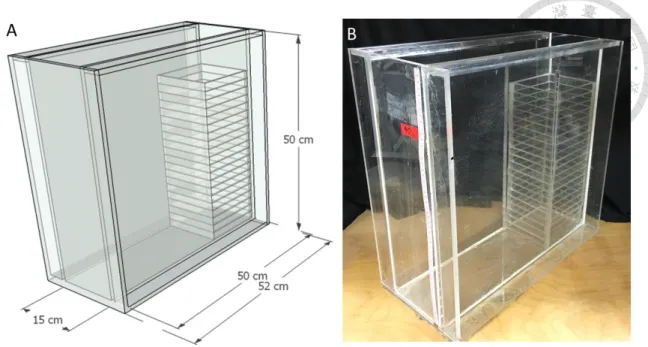
The size of the tank (Fig. 3.1) is designed according to the requirement of shear strength experiment and the detailed reason would be explained in section 3.3.2.

The fine sediment used in experiments is obtained from the near dam bottom of Tsengwen Reservoir in southern Taiwan. The properties of sediment are listed as follow.

(31)

Fig. 3.1 Tank: (A) sketch and size (B) photo

Table 3-1 Sediment properties

Property Value Unit

The density of mixing silt and clay(_S) 2.7 _{g cm}³

Plastic limit (PL) 19

Liquid limit (LL) 35

Plasticity index (PI) 16

Median diameter (D ) ₅₀ 0.0079 mm

To make sure the self-weight consolidation experiments start from the same initial condition, there are three steps to prepare the sediment sample. First, mix the sludge with water by electric drill until the density of sediment sample being 1.26g cm³ which is measured by hydrometer (Fig. 3.2 (A) ,(B) and (D)). Next, filter the mixture through the sieve to remove small twigs, stones and other impurities (Fig. 3.2 (C)). Last, fill the sediment sample into the tank up to the depth reaching 40 cm .

(32)

Fig. 3.2 Sediment sample preparation procedure: (A) mixing (B) measuring (C) filtering (D) hydrometer.

(33)

3.2 Settlement

3.2.1 Experimental Material and Procedure

The materials this experiment requires are tank and sediment sample which have mentioned in previous section. The experimental procedure is simple that only needs to record the height of mud surface every day (Fig. 3.3). Then, the difference between original depth (40 cm ) and mud surface is the settlement value which is of interest.

Fig. 3.3 The mark of record

(34)

3.2.2 Experimental Results

Fig. 3.4 Relation between consolidation duration and elevation

Based on the result of experiment, the settlement shows as exponential curve along with time. In previous 5 days, the elevation declines dramatically. From 6 to 15 days, the range of decrease tends to be gradual. After 15 days, there is no obvious reduction.

Fig. 3.5 Relation between consolidation duration and degree of consolidation

(35)

The definition of degree of consolidation (U) is ( ) ( )

max

U t S t

 S (3.1)

where S_max is the maximum settlement; S is the settlement at that time.

The settlement on 30 days acts as the maximum settlement. Therefore, the value of degree of consolidation is from 0 to 1 along with time. The value that closer to 1 means higher consolidation degree. Furthermore, the curve of degree of consolidation is vertically symmetrical with the curve of settlement.

3.3 Shear Strength

3.3.1 Introduction

“The shear strength of a soil mass is the internal resistance per unit area that the soil mass can offer to resist failure and sliding along any plane inside it.” ( Das, B. M.,

& Sobhan, K., 2002: 311) There are some conventional tests to measure the shear strength. In laboratory test, the common tests are quick shear test, consolidated quick shear test and slow shear test. On the other hand, vane shear test and cone penetration test are familiar for in situ test.

However, the conventional tests are not suitable for self-weight consolidation experiments we conducted because the shear strength of mud is too small to measure. In brief, the mud in this experiment is too soft. The existing tests are usually used by geotechnic field that care about large scale issue. To solve the problem, an in situ test which is called T-bar penetration test is improved to adapt the situation (Newson et al., 1983).

(36)

3.3.2 Experimental Material, Setup and Procedure

There are 4 main materials in the experiment: (i) a soil triaxial tester, (ii) a T-bar, (iii) a load cell, and (iv) tanks.

The foundation used in this experiment is soil triaxial tester produced by the company, HUMBOLDT (Fig. 3.6). The lifting platform with diameter of 15 cm is used to place the tank with sediment sample and goes up and down. Display screen shows the value that load cell measures. Computer beside is used for data record. Besides, because the diameter of lifting platform is 15 cm , the wide of tank is also designed as 15 cm to confirm it be stable.

Fig. 3.6 Soil triaxial tester

(37)

T-bar is composed of stainless steel pipes and the size of it is consulted from DeGroot et al. (2010). (Fig. 3.7 (A) and (C)). Moreover, the other two shorter stainless steel pipes are used to lengthen the T-bar. Because the lifting platform is only able to rise 10 cm , the two shorter pipes are connected to let T-bar reach deeper. The connection is shown in Fig. 3.7 (B) in detail.

Fig. 3.7 T-bar: (A) photo (B) connection (C) sketch and size

The S load cell produced by the company, esense (Fig. 3.8). The capacity is decided as 2 kg through several tests. As a matter of fact, too large capacity makes the load cell less accurate. On the contrary, too small capacity causes the load cell to overload and be broken. Therefore, we cannot emphasize the importance of choosing the capacity of a load cell too much. Moreover, the S load cell can measure tension and compression both.

(38)

Fig. 3.8 S load cell: (A) photo (B) sketch and size

Table 3-2 Specification of S load cell

Property Value Unit

Capacity 2 kg

Safe overload rating 150 %

Rated output 2.0 mV/V

Total error 0.05 %

Repeatability 0.03 %

Creep 0.05 % / 30min

The setup photo of shear strength experiment is shown in Fig. 3.9. The S load cell is fixed at the frame of soil triaxial tester and connected with T-bar below. The tank is placed on the lifting platform. It should be cautious that the T-bar cannot touch the surface of sediment sample or it would affect the initial condition of experiment.

Moreover, according to the recommendation of DeGroot et al. (2010) which states that the velocity of lifting platform should be 0.5 diameter of T-bar per second; therefore, the velocity is decided to be 1 cm s ( the diameter of T-bar is 2.19 cm ).

(39)

Fig. 3.9 Setup of shear strength experiment: (A) photo (B) interpretation

The experimental procedures are as follow:

Step 1: stand the sediment sample for expected consolidation duration (Fig. 3.10 (A)).

Step 2: on the expiration day, place the tank with sediment sample on the lifting platform.

Step 3: install S load cell and T-bar as mentioned above.

Step 4: configure parameters of soil triaxial tester.

Step 5: press button to let the lifting platform keep going up to its limit 10 cm . The data is recorded each 0.1 cm in the meantime (Fig. 3.10 (B) and (C)).

Step 6: disassemble the connection with S load cell and T-bar.

Step 7: let the lifting platform go downward 10 cm and fix the T-bar at the same time.

Step 8: connect the shorter stainless steel pipe with T-bar in order to lengthen it.

Step 9: repeat Step 5 to Step 8 until T-bar is at 3 cm from the bottom of tank.

(40)

Step 10: repeat Step 5 to Step 9. Differently, the lifting platform goes downward instead of upward because the purpose is to let T-bar pull out from the sediment sample and also measure the value.

Step 11: save the recorded data.

Fig. 3.10 Procedure of shear strength experiment: (A) stand the sediment sample for consolidation duration. (B) let lifting platform go upward. (C) A close look when T-bar

is pushed in the sediment sample.

(41)

Before conducting the experiment, the S load cell needs to be calibrated to make sure its accuracy. The results are illustrated in Fig. 3.11. The equations of fitting curve show that the testing values are very close to the true values which means the S load cell is able to measure the loading correctly and accurately.

Fig. 3.11 Calibration: (A) compression (B) tension

3.3.3 Data Analysis and Interpretation

The analysis and interpretation of experimental data to estimate shear strength is introduced in this chapter. The process is referred to journal papers based on current understanding.

First of all, there are three types of calculation to deal with the readings derived from the S load cell and they are introduced as follow:

Type I: the readings ( R ) act as the loadings (L ). Neglect the behavior of buoyance. _I

RLI (3.2)

Type II: the readings obtaind from the S load cell subtracte buoyance of T-bar to get the

(42)

loadings (L ) of S load cell. The buoyance (_II B ) is estimated as _I ( ) ( )

I W

B z   z  g (3.3)

where  is the volume of T-bar which is in the fluid; _W is the density of water and the value of it is 1g cm³; g is the gravity.

It is worth to be mentioned that the density of fluid here is simplified to take as constant (1g cm³).

Then, the readings subtracte buoyance calculated above to get the loadings (L ) of S _II load cell.

I II

R B L (3.4)

Type III: the buoyance (B ) is derived as _II

g p

   (3.5)

( g ,_x g ,_y g )_z ( p, p, p) x y z

   ^{  }

  

   (3.6)

We are interested in the pressure of x direction and define P( ,0,0)p , then ( ) (( ,0,0) (n , n , n ))_x _y _z ( n ) dA_x

s s s

P n dA  p  dA p

  

^(3.7)

By Gauss’s theorem

( n) ( ) (( , , ) ( ,0,0)) ( )

s

P dA P d p d p d

x y z x

  

   

        

   

   

^(3.8)

Based on equation(3.6), equation(3.8) can be showed as

( p) ( g )_x _px 0

d d F

x 

 

      







^(3.9)

Next, We are interested in the pressure of y direction and define P(0, ,0)p , then (P n dA )  ((0, ,0) (n , n , n ))p  _x _y _z dA ( n ) dAp _y

  

^(3.10)

(43)

( n) ( ) (( , , ) (0, ,0)) ( )

s

P dA P d p d p d

x y z y

  

   

        

   

   

^(3.11)

( p) ( g )_y _py 0

d d F

y 

 

      







^(3.12)

Last, We are interested in the pressure of z direction and define P(0,0, )p , then ( ) ((0,0, ) (n , n , n ))_x _y _z ( n ) dA_z

s s s

P n dA  p  dA p

  

^(3.13)

( n) ( ) (( , , ) (0,0, )) ( )

s

P dA P d p d p d

x y z z

  

   

        

   

   

^(3.14)

( p) ( g )_z _pz

d d F

z 

 

     







^(3.15)

Thus, the buoyance (B ) can be expressed as _II

p pz II

F g d p d F B

 





   



   ^(3.16)

g ( ) g ( ) g ( )S(z) g

pz z

F  d  z d  z dxdydz  z dz

   





 



 







^(3.17)

where

( )

S z

S z 



dxdy^.

Therefore, based on equation(3.17), the density of type III is variable with the depth which is applied to the experiment more appropriately since the fluid density changes with the depth. Then, the readings subtract the corresponding buoyance (B ) to yield _II the loadings (L ). _III

(44)

II III

R B L (3.18)

Secondly, let loadings ( L ) divide by the cross section of T-bar ( A ) which touches the sediment sample

T bar

q L

  A (3.19)

where q_{T bar}_ is the initial net resistance for T-bar [N m²]; the value of A is 0.125 0.02 [ m2] according to the size of T-bar.

Last but not least, shear strength (S_u) is estimated as the ration of initial net resistance to a shear strength factor (N_{T bar}_ )

T bar u

T bar

S q N



 (3.20)

As a matter of fact, the value of N_{T bar}_ is related to surface roughness and the in situ state. In practice, the shear strength factor is found from an upper and lower bound plasticity solutions (Randolph and Houlsby, 1984). An average value of 10.5 is used typically (Stewart and Randolph, 1994). Therefore, 10.5 is chosen as the value of shear strength factor for T-bar in this experiment.

Moreover, there are various manners to estimate the relation among initial net resistance, shear strength and shear strength factor. Some states that it is also related to initial total vertical stress and hydrostatic pore pressure. Some suggests that the total overburden pressure and pore water area correction factor should be taken into account.

However, to simplify, equation(3.20) is used in this experiment.

(45)

Fig. 3.12 Three types of buoyance calculation for 1 day

Fig. 3.13 Three types of buoyance calculation for 3 days

(46)

(47)

Fig. 3.12 to Fig. 3.16 are the comparisons among the three types of buoyance calculation for the different consolidation duration. It is clear that the value of type I is the largest since it does not subtract the buoyance. Besides, the value of type III is smaller than type II and the reason is that the density of type III changes with the depth which is bigger than 1g cm³ yet the density of type II remains at 1

g cm3. Moreover, the difference between the latter two is within 10N m² . Furthermore, type III is the most thorough and exhaustive method to estimate the behavior of buoyance, hence it is chosen as the method to obtain loadings.

(48)

3.3.4 Experimental Results

Fig. 3.17 Shear strength for 1 day

Fig. 3.18 Shear strength for 3 days

(49)

(50)

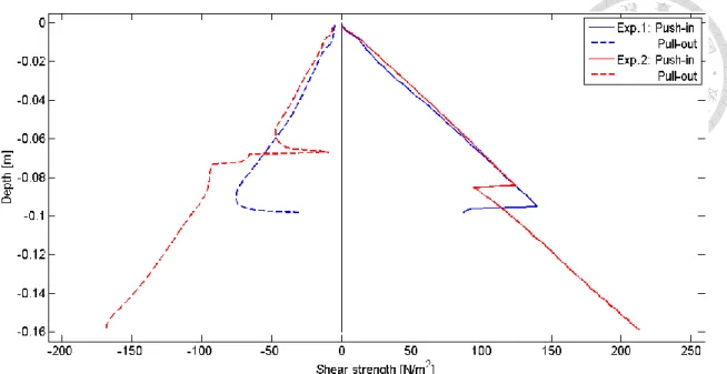
Fig. 3.17 to Fig. 3.21 are the results of shear strength for 1 day, 3 days, 7 days, 14 days and 30 days, separately. The solid lines represent push-in of T-bar and dotted lines represent pull-out of T-bar. The experiments are conducted by T-bar with and without extension both, hence there are two different depths of every consolidation duration.

However, it is worthwhile to note that the pull-out results of Exp.3 for 3 days has some problems.

Fig. 3.22 Comparison of Shear strength for different consolidation duration

(51)

Based on Fig. 3.22, there is no denying that the longer the consolidation duration is, the larger the shear strength is. Moreover, the shear strength increases as the depth increases and the phenomenon is more obvious in long consolidation duration.

3.4 Layer Density

3.4.1 Experimental Material, Setup and Procedure

The materials used in this experiment are tank, sediment sample and acrylic layers.

Tank and sediment sample have been introduced in previous section. Moreover, an acrylic layer is composed of four acrylic plates and the size is illustrated in Fig. 3.23.

Fig. 3.23 Sketch of acrylic Layer

The experimental preparation is almost the same as settlement experiment which only add a step. Before filling the sediment sample into the tank, 20 acrylic layers are piled in the tank first (Fig. 3.24). Each acrylic layer is 2 cm high and the depth of sediment sample is 40 cm , hence it needs 20 acrylic layers to be as high as sediment sample. Then, stand it for consolidation duration as plan (Fig. 3.25).

(52)

Fig. 3.24 Tank with acrylic layers: (A) sketch and size (B) photo

Fig. 3.25 Standing the tanks for expected consolidation duration

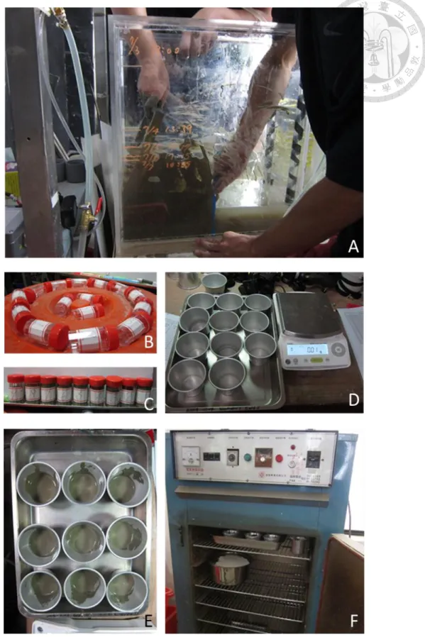
On the expiration day, the sediment sample is going to take out to measure its density of each 2 cm layer. To begin with, use a sampling bottle which is labeled number (Fig. 3.26 (B)) to dig a lump of sediment and carefully do not dig the sediment too deeper which belongs to next layer. Secondly, take out the top acrylic layer slowly and push the sediment sample in it to the other side (Fig. 3.26 (A)). Besides, keep

(53)

removing sediment sample on the other side to make sure the depth of it is not higher than acrylic layers. Repeat the above steps until 20 acrylic layers all move out. Then, place an empty aluminum bowl (m_b) which is also labeled number on electronic scale to get its weight (m ) (Fig. 3.26 (D)). Next, pour out the sediment in sampling bottle to _b the aluminum bowl and weigh them again (m_bm_sm_w). Repeat weighing the rest of aluminum bowls and sediment sample (Fig. 3.26 (E)). Furthermore, put the aluminum bowls with sediment sample in the oven one day to dry them (Fig. 3.26 (F)). Last, weigh the aluminum bowl with dry solid (m_bm_s) and the density of each layer (_L) is calculated as follow:

s w

L

s S w W

m m

  

 

 (3.21)

where _S is the density of dry solid and the value of it is 2.7g cm³; _W is the density of water and the value of it is 1g cm³.

(54)

Fig. 3.26 Layer density experimental procedure: (A) acrylic layer removal (B) empty sampling bottles (C) sampling bottles with sediment (D) weighing (E) aluminum bowls

(55)

3.4.2 Experimental Results

Fig. 3.27 Layer density profile for 1 day

Fig. 3.28 Layer density profile for 3 days

(56)

(57)

Fig. 3.32 Time evolution of the density profile

(58)

Fig. 3.27 to Fig. 3.31 are the results of layer density for each consolidation duration which contains at least two experiments. In the same duration, different experiments present the similar density distribution profile. Moreover, the differences among different experiments in 1 day and 3 days are larger than in 7 days, 14 days and 30 days.

The curves in Fig. 3.32 are the average values of different experiments of each duration which have mentioned above. According to Fig. 3.32, all curves reveal that the density grows with depth increases. Besides, at the same density, the longer the consolidation duration is, the higher the elevation is. Moreover, at the same elevation, the density increases with consolidation duration gains. Furthermore, the density no longer increases at the lower elevation from 14 days to 30 days.

(59)

(60)

Chapter 4 Comparison

4.1 Calibration of Parameters

In order to compare the theory with the experiment, it is necessary to calibrate the parameters,c ,_v a and_v N_strength, in the theory.

Coefficient of consolidation (c ) is the parameter which controls the consolidation _v duration. That is, c dominates the settlement curve when to drop to a plateau. To fit _v in with the experimental result, the value of c is decided to be _v 2.7 10 ^⁷ (m s² ).

Coefficient of compressibility (a ) is the parameter which controls the settlement _v amount. However, when a is adjusted to match up the experimental results, the value _v of volumetric concentration (c ) would be bigger than 1 which is not feasible and the _s reason is the value of a , according to equation(2.15) and (2.16). Consequently, to _v reach a balance between c and _s a , _v a is chosen to be _v 0.4 10 ( ^² m N² ).

Empirical factor of shear strength (N_strength) is the ration between effective stress and shear strength (equation(2.30)). Compared with the experimental results, N_strength is decided to be 0.22.

(61)

4.2 Compare Theory with Experiments 4.2.1 Settlement

Fig. 4.1 Settlement comparison

According to the aforementioned, the experiment and theory cannot match up well in settlement. Fig. 1.1Fig. 4.1 illustrates that the trend of both are similar, yet the settlement amount exists difference. The dominant reason is that Terzaghi’s theory of one-dimensional consolidation applies to small strain. However, the settlement of experiment we conducted belongs to large strain. Even so, because Terzaghi’s theory is not complicated as other theory, it is still used to simulate the consolidation phenomenon.

(62)

4.2.2 Shear Strength

Fig. 4.2 Shear strength comparison for 1 day

Fig. 4.3 Shear strength comparison for 3 days

(63)

(64)

Fig. 4.7 Shear strength comparison of theory with experiment for all duration Fig. 4.2 to Fig. 4.6 are shear strength comparisons for different consolidation duration and Fig. 4.7 is the combined version. The trends of both are approximately the same. In the cases of 1 day, 3 days and 7 days, the concaves are all upward which means

(65)

they all present as straight lines that fit in with physical mechanism which has mentioned before. Moreover, the values of theory are bigger than experiment and the phenomenon is more obvious in short consolidation duration.

4.2.3 Layer Density

Fig. 4.8 Layer density comparison for 1 day

Fig. 4.9 Layer density comparison for 3 days

(66)

(67)

Fig. 4.13 Layer density comparison of theory with experiment for all duration

(68)

Fig. 4.8 to Fig. 4.12 are layer density comparisons for different consolidation duration and Fig. 4.13 is the combined version. The results of experiment and theory fit in with each other well in short consolidation duration. However, in long consolidation duration, the concave of experiment is downward, but the concave of theory is upward.

The condition is observable in equation(2.15) that the relation between shear strength and layer density are linear, hence the trends of both are the same.

In order to make sure the conjecture is correct, the relation between shear strength and void ratio of theory is compared to experiment. The results are illustrated in Fig.

4.14 to Fig. 4.16. According to the result, the relation between shear strength and void ratio of theory is linear, yet the relation of experiment shows as exponential distribution.

It is obvious that the relations of theory and experiment are different. In other words, the relation we build in theory (equation(2.15)) is not suitable for the reality. To solve the problem, it should be brought another formula to construct the relation.

Fig. 4.14 Theory and experiment comparison of the relation between shear strength and void ratio

(69)

Fig. 4.15 Theory and experiment comparison of the relation between shear strength and void ratio from 1 to 5

Fig. 4.16 Theory and experiment comparison of the relation between log shear strength and void ratio from 1 to 5

(70)

Moreover, some state that the consolidation does not start from the initial condition but after a few days. In first few days, the distance between particles reduces which is called sedimentation but the behavior does not increase the shear strength. The consolidation begins after it. Besides, from Fig. 4.7, it is observable that the shear strength for 1 day and 3 days gains little in upper elevation. The phenomenon reveals that the statement mentioned above is feasible in this case; therefore, the consolidation duration is delayed 1 day for theory calculation.

Fig. 4.17 Settlement comparison after delaying consolidation duration

(71)

Fig. 4.18 Shear strength comparison after delaying consolidation duration

Fig. 4.19 Layer density comparison after delaying consolidation duration

For this try, it is assumed that the consolidation process starts from second day.

Based on Fig. 4.17 to Fig. 4.19, the elevation of settlement begins at 32 cm which is the height of second day. The results show that the settlement of theory fit experiment better than no delay. Moreover, the results of shear strength and layer density both are

(72)

acceptable.

To sum up, to improve the consolidation theory, there are two ways to conduct: (i) developing a feasible relation between effective stress and void ratio, and (ii) separating the whole process into two parts. The first part is sedimentation for the first few days and the second part is consolidation after it.

(73)

(74)

(75)

(76)

Chapter 5 Experiments

5.1 Introduction

To simulate the sediment removal of hydrosuction in reservoir, a series of experiments are conducted to compare different conditions to try to find out the most efficient way of sediment removal. First, experimental setup and materials are introduced one by one in detail. Next, in order to address the long consolidation duration problem, the reduced scale and simplified external force equipment is designed to simulate the prototype applied in field site. Finally, the experimental procedure is listed.

5.2 Experimental Material and Setup

The conceptual sketch and photo of experimental setup are shown below (Fig. 5.1

& Fig. 5.2). The main elements are (i) a tank, (ii) a constant head water supply tank, (iii) an energy dissipation box, (iv) a vertical screw, (v) a horizontal linear slide, (vi) a hydrosuction pipe, and (vii) a densimeter. Each of elements would be introduced in detail.

(77)

Fig. 5.1 Conceptual sketch of experimental setup

Fig. 5.2 Photo of experimental setup

(78)

The tank is 100 cm long, 30 cm wide, and 50 cm high and made up of acrylic plates (Fig. 5.3). There are 5 tanks being stood for different consolidation duration and the initial depth of sediment sample is 40 cm. Besides, there is an open for overflow at

47 cm in each tank to make the water level fixed during experiment process (Fig. 5.4).

Fig. 5.3 Tank

Fig. 5.4 Open for overflow

(79)

The water supply tank is designed for overflow to maintain the same water level.

Consequently, the supplied water is constant head (Fig. 5.5). Then, the water is conveyed form water supply tank to energy dissipation box the objective of which is to decrease the influence of water inflow in order to avoid agitating the consolidated sediment sample (Fig. 5.6).

Fig. 5.5 Constant head water supply tank

Fig. 5.6 Energy dissipation box

(80)

The hydrosction is a copper pipe with internal diameter of 0.8 cm. The function of hydrosuction pipe is to withdraw slurry by siphoning. The full pipe condition starts by the vacuum pump (Fig. 5.8) to draw out the air in the pipe to make it fill with water.

Fig. 5.7 Hydrosuction pipe

Fig. 5.8 Vacuum pump

以淤泥實驗探討壓密、射流、擾動及水力抽砂行為之研究

國立臺灣大學工學院土木工程學系 碩士論文

Department of Civil Engineering College of Engineering National Taiwan University

Master Thesis

以淤泥實驗探討壓密、射流、擾動及水力抽砂行為之研究 Consolidation, jetting, stirring and hydrosuction of

experimental mud deposits

葉亭霞 Ting-Sia Ye

指導教授：卡艾瑋 教授 Advisor: Dr. Hervé Capart

中華民國 105 年 7 月

July, 2016

誌謝

中文摘要

ABSTRACT

CONTENTS

LIST OF FIGURES

LIST OF TABLES

Chapter 1 Introduction

Chapter 2 Theory

2.1 Framework of Theory

 

 

2.2 Solution









Let





2.3 Results

Chapter 3 Experiments

3.1 Introduction

3.2 Settlement

3.2.1 Experimental Material and Procedure

3.2.2 Experimental Results

3.3 Shear Strength

3.3.1 Introduction

3.3.2 Experimental Material, Setup and Procedure

3.3.3 Data Analysis and Interpretation

  

   





  

   





  

   



















3.3.4 Experimental Results

3.4 Layer Density

3.4.1 Experimental Material, Setup and Procedure

3.4.2 Experimental Results

Chapter 4 Comparison

4.1 Calibration of Parameters

4.2 Compare Theory with Experiments 4.2.1 Settlement

4.2.2 Shear Strength

4.2.3 Layer Density

Chapter 5 Experiments

5.1 Introduction

5.2 Experimental Material and Setup

國立臺灣大學工學院土木工程學系碩士論文

指導教授：卡艾瑋教授 Advisor: Dr. Hervé Capart