PD Control of a Constrained Flexible Arm via Parallel Compensation
Liang-Yih Liu
1, Hsiung-Cheng Lin
21Department of Electrical Engineering, Chienkuo Technology University, Taiwan
2Department of Electronic Engineering, National Chin-Yi University of Technology, Taiwan
1[email protected], 2 [email protected]
Abstract
In this paper, the force control of a constrained one- link flexible arm is investigated using a linear distributed parameter model, including internal damping of Kelvin-Voight type. To overcome the inherent limitations caused by the non-minimum phase nature of the noncollocation from the joint torque input and the tip contact force output, a new input induced by the root bending moment, and a contact force output generated by a parallel compensator are defined. The transfer function from the new input to the contact force output proves that it is not only strictly minimum phase but also a stable condition. A PD controller is then designed to improve the performance of the overall closed loop system. It is shown that asymptotic tracking of a desired contact force trajectory with internal stability can be achieved accurately. In order to obtain exact solutions of the infinite-dimensional system, the infinite product formulation is used throughout the paper. Numerical simulations are provided to verify the effectiveness of the proposed approach.
Keywords: constrained flexible arm, parallel compensator, minimum phase system, infinite- dimensional system.
Introduction
Force control of constrained flexible manipulators has received an increasing attention in recent years [1-8].
Application of this research field include space robots used for satellite capturing and large space structure construction, and light weight industrial robots used for assembly, deburring and grinding tasks. The controller design for such force control problems is, however, quite difficult due to the distributed parameter nature of flexible arms and the noncollocation of torque actuation and contact force sensing.
Several methods have been proposed for force control of constrained flexible manipulators. Based on finite-dimensional approximate models, Chiou and Shahinpoor [1-2] studied a single-link and a two- link constrained flexible manipulators, and pointed out that the link flexibility is the main source of dynamic instability of the force controlled systems.
Later, in [3], Li indicated that an inherent limitation on
the achievable bandwidth of force control occurs due to the presence of infinitely many non-minimum phase zeros. It is known that the flexible arm is inherently infinite-dimensional system in nature. As a result, the design of the finite-dimensional controller for the constrained one-link flexible arm may become more complicated using the distributed parameter model.
Obviously, this phenomenon posted a difficulty for such a model to be realized. Somehow, the problem was overcome using the Lyapunov method by Morita et al. [4] and Endo et al. [5]. The asymptotic stability of the closed-loop system was also achieved. But the proposed method may not guarantee the constrained one-link flexible manipulator system to be stable.
Recently, the passivity-based PD control using the infinite product formulation presented a satisfactory performance outcome in the linear distributed parameter model [6] However, the internal material damping was not considered in this study by Liu and Yuan [6. In the recent advanced progress, Bazaei and Moallem [7] proposed a distributed parameter model for a constrained flexible beam actuated at the hub, achieving the maximum control bandwidth. Bazaei and Moallem [8] extended their work to improve force control bandwidth of the constrained one-link arm through output redefinition. Unfortunately, the suppression of high frequency modes may pay a high cost because of degrading the performance attainable.
To overcome the limitations of above papers, this paper is to develop the asymptotic tracking of a desired contact force trajectory, being achieved using a distributed parameter model of the constrained one-link flexible arm. In order to reflect the intrinsic property of internal friction of the link material, a distributed parameter model which includes the widely used Kelvin-Voight damping has been considered. To remove the nonminimum phase obstacle relating the joint torque input and the tip contact force output, a new input induced by the root bending moment and its derivative, and a virtual contact force output generated by a parallel compensation are defined. It will prove that the transfer function from the new input to the virtual contact force output has all its infinite number of poles and zeros lying in the open left-half plane. Then, a PD control is used to improve the performance of the
infinite dimensional closed loop system. To preserve the exact poles and zeros of the system, the infinite product representations of transfer functions are employed throughout the paper. Numerical simulations are presented to demonstrate the excellent performance of the proposed approach.
Dynamic model
Derivation of Equations of Motion
The constrained one-link flexible arm depicted in Figure 1 is a uniform, homogeneous, Euler-Bernoulli beam of length , mass per unit length , and flexural rigidity EI . The hub is modelled by a single-mass moment of inertia Ih where the driven torque(t) is applied. The end-effector has a concentrated mass mp, where the contact force exerted by the smooth rigid constraint surface is (t) . The cd 0 is a small damping constant of the beam material.The arm is assumed to move in a horizontal plane so that the gravity can be ignored. Let the X-axis be a fixed frame and x-axis be a floating frame, both coincident with the neutral axis of the beam. The hub angular displacement
)
(t is defined as the counterclockwise rotation of the x-axis with respect to the X-axis. Let v(x,t) be the small transverse deflection of the neutral axis of the beam with respect to the x-axis.
Ih
( )t
( )t v x t( , )
mp
( )t
X x
x u(x,t)
Figure1. Schematic of a constrained flexible arm The equations of motion and the corresponding boundary conditions are (the details are rather involved and thus omitted)
( ) ( ) ( , ) ( ) ( )
0
t t dx t x v t x x t
Ih
(1)
x(t)v(x,t)
EIvxxx(0,t)cdEIvxxx(0,t)0 (2)
0 ) , 0 ( t
v (3)
0 ) , 0 ( t
vx (4)
0 ) , ( )
,
( t c EIv t
v
EI xx d xx (5)
) ( ) , ( )
,
( t c EIv t t
v
EI xxx d xxx (6)
Substitute Eqs. (2) and (6) into (1), and perform integration by parts with Eq. (5), an alternative form for Eq. (1) is obtained:
) ( ) , 0 ( )
, 0 ( )
(t EIv t c EIv t t
Ih xx d xx (7)
The root bending moment vxx(0,t) can be measured by a strain gauge sensor [4,8] and its derivative vxx(0,t) can be detected by a full- bridge strain gauge [8]. This enables one to introduce a new joint input variable u(t) such that
) ( )
(t I t
u h (8)
Non-Minimum phase transfer function from the input torque to the contact force
The transfer function can be derived by taking the Laplace transform of Eqs. (2)-(8) assuming zero initial conditions. Let s be the Laplace transform variable, and define the dimensionless parameters ,
, , , and sˆ as
cd
EI 2
1
4
,
3
Ih , s EI s
2 1 4
ˆ
(9)
s
s s s c
EI d 1 ˆ
ˆ 1
2 2 4 4
(10) With the application of infinite product representation of transcendental functions given in the Appendix, The results are (bearing in mind the implicit relation between s and defined by Eq.(10)) as follows
) cos sinh sin (cosh sin
sinh 2
sin sinh ˆ)
( ˆ) : ( ˆ)
( 3
s
s s G
1
2 2 1
2 2
ˆ ˆ 1
ˆ ˆ 1 1
n n
n zn
s s s s
(11)
cos sinh cosh sin
sin sinh 1
ˆ) (
ˆ) : ( ˆ)
( 2
s u s s G u
1
2 2 1
2 2
2 ˆ
1 ˆ ˆ ˆ 1
ˆ ˆ 1 3
n n
n zn
s s s s
s s
(12)
cos sinh cosh sin
) cos sinh sin (cosh sin
sinh 2 1 ˆ) (
ˆ) : ( ˆ) (
3
3
s u s s G u
1
2 2 1
2 2
2 ˆ
1 ˆ ˆ ˆ 1
ˆ ˆ) 1 ( 3
n n
n n
s s s s
s s
(13)
where zn and n n are defined in the Appendix.
The numerical values of n() can be computed using n n2, where n(), n1,2 are the real positive roots of the denominator of Eq. (11), namely
0 ) cos sinh sin
(cosh sin
sinh
2 3 (14)
Table 1 reveals the results of selected values of n. Note that the poles and zeros of G( sˆ) are, respectively, given by
, 2 , 1 4 ,
2 ˆ
2 2 2
n
s
n n
(15)
and
, 2 , 1 4 ,
2 ˆ
2 2 2
n
s
n z n
z
(16)
1 ˆ1 s
ˆ) Re( s
n Re( sˆ)
ˆ) Im( s
1
2
n
n n
ˆ) Im( s
Figure 2. (a) Distribution of poles of G( sˆ), and (b) distribution of zeros of G( sˆ)
The distribution of these poles and zeros on the complex sˆ-plane are shown schematically in Figure 2.
Since G( sˆ) has infinitely many zeros in Re(sˆ)0, ˆ)
( s
G is a nonminimum phase. Similarly, Gu( sˆ) is also a nonminimum phase. The effect of introducing the new input u(t) via root bending moment and its derivative is merely to change the poles of G( sˆ) to the poles of Gu( sˆ).
Controller design
Removing the non-minimum phase obstacle by parallel compensation
Table 1 Values of roots of associated transcendental equations
To alleviate the non-minimum phase problem, the right half-plane zeros can be replaced by the left half- plane zeros by the method of redefinition of output.
Define a new virtual contact force f(t,k) such that
cos sinh cosh sin
) cos cosh 1 ( ) 1 ( ) sinh (sin 1
ˆ) (
) ˆ, : ( ) ˆ, (
2
k k
s u
k s k f s Gfu
(17)
where k is a real constant. It was shown in [9] that for k0.758 , one can write
1
2
ˆ2
1 ˆ 1 1 2
) cos cosh 1 ( ) 1 ( ) sinh (sin
n n
s s
k k
(18)
The numerical values can be computed using
2 n
n
, where n( k) , n1,2 are the real positive roots of the numerator of Eq. (18). Selected values of n are listed in Table 1. Thus, one has a minimum phase stable transfer function
n
n(k 0.7)
n
( 2.557 10 )
1
n
1 2.8472 4.9002
1.8162
2 4.0822
7.7252
3.9922
3 8.1452 11.0862
7.0802
4 10.7772 14.0662
10.2142
5 14.3012 17.3362
13.3532
6 17.1422
20.3712
16.4942 7 20.5342
23.6042
19.6352 8 23.4632
26.6662
22.7772
odd n
2
) 2 ( 1 3 ) 7 2 ( 1
n n
2
) 2 ( 1 ) 1 2 ( 1
n n
even n
2
) 2 ( 1 3 ) 7 2 ( 1
n n
2
) 2 1 ( ) 1 2 ( 1
n n
2
3
)3
4 ( 3
9108 . ) 3 4 ( 3
n n
1
2 2 1
2 2
2 ˆ
1 ˆ ˆ ˆ 1
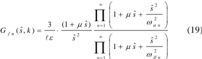
ˆ ˆ) 1 ( ) 3 ˆ, (
n n
n n
u f
s s s s
s k s
s G
(19)
where the distribution of poles and zeros of )
ˆ, (s k
Gfu takes similar pattern as shown in Figure 2(a).
Note that the above redefinition of output is equivalent to the parallel compensation [10] as shown in Figure 3(a). It can be shown that the parallel compensator
) ˆ, (s k
T has the form
cos sinh cosh sin ) sinh (sin
) cos cosh 1 ( ) 1 ) ( ˆ,
( 2
k k s T
1
2 2 1
2 2
ˆ ˆ 1
ˆ ˆ 1
40 ) 1 ( 11
n n
n n
s s s s k
(20)
where n n2 and n( k) , n1,2 are the real positive roots of the equation
0 ) sinh (sin
) cos cosh 1
(
(21)
Selected values of n are computed and listed in Table 1.
PD Control of the Parallel Compensated System For the control structure as shown in Figure 3(a), the objective is to make (t) to track asymptotically a desired contact force trajectory d(t) using an PD control, where kp and kd are positive design constants, and k0.758 . Obviously
ˆ) ( ) ˆ, ( ˆ) (
1
ˆ) (
) ˆ,
( s
k s G s k k
s k k k
s
u d
u f d p
d
p
(22)
The characteristic equation of the closed-loop system is 0
) ˆ, ( ˆ) (
1 kpkds Gfu s k (23) To ensure that asymptotic tracking of output trajectories can be achieved even in the absence of internal damping. With Gfu(sˆ,k) given by setting
0
in Eq. (19), Eq. (23) becomes
1 ˆ
ˆ 1
ˆ 1 ˆ)
( 3
1
2 2 2
1
2 2
n n
n n
d p
s s
s
s k k
(24)
Figure 3. (a) PD control of parallel compensated system;
(b)overall closed-loop system in basic feedback loop Clearly, the effect of P-control alone is merely to move all the closed-loop poles along the imaginary sˆ- axis from sˆ j,n1 (set 0 0) to sˆ jn ,
, 2 ,
1
n as kp varies from 0 to . With kp k*p, Eq. (19) can be rewritten as
N
s s s
k k
N
n n
N
n n
p
d 1,
ˆ 1
ˆ ˆ 1
1
1 2 2 1
2 2
*
(25)
It can be easily verified using a simple root locus plot that the D-control suffices to stabilize the closed- loop system for all 0k*p and 0kd . Therefore, it is reasonable to conjecture that the damping effect should be enhanced when internal damping are considered. Let the roots of Eq. (23) be written as
, 2 , 1 ,
ˆ 1 2
4
s j n
EI
sn n nn n n
(26) where n(n n1) and n are the natural frequency and damping ratio of the n-th closed-loop pole. Using Eq. (19), one may write Eq. (23) as
N
n n
N
n n
d p
s s s s
s s
s k k
1
2 2 2
1
2
2 ˆ
1 ˆ ˆ ˆ
1 ˆ ˆ) 1 ˆ)(
( 3
s N k s
N
n n n
n
p ˆ ˆ ,
2 1 3
1
1
2 2
(27)
(a)
(b)
Using Eq. (22) foru(sˆ,k) andGu( sˆ), Gu( sˆ) given by Eqs. (19) and (12)-(13), the closed-loop responses of some relevant variables can be computed as follow.
s N
s s
s s s
s k
s k d
N
n n n
n N
n zn
p
d (ˆ),
ˆ ˆ 2 1
ˆ ˆ 1 ˆ) 1 ( 1 ˆ ˆ)
( 1
1
2 2 1
2 2
(28)
s N
s s
s s s
s k
s k d
N
n n n
n N
n n
p
d (ˆ),
ˆ ˆ 2 1
ˆ ˆ 1 ˆ) 1 ( 1 ˆ ˆ)
( 1
1
2 2 1
2 2
(29)
Note that the above results are exact closed-loop solutions of the infinite-dimensional force control system. To perform the inverse Laplace transform,sˆcan be replaced by s
EI
4
. The closed- loop time responses can be computed within an arbitrary degree of accuracy by taking N as large as required. In order to find the exact values (to the extent of numerical accuracy) of the closed-loop poles (i.e. the roots of Eq. (23), Gfu(sˆ,k) given by Eq. (17)
must be used. Using either of 4
1 2
1 ˆ ˆ 2 1
s s j
, the
equation
0 sin
cosh sinh cos
) cos cosh 1 ( ) 1 ( ) sinh ) (sin
ˆ (
1 2
k s k
k kp d
(30) can be solved numerically to yield n and
n,n1,2. The control structure of Figure. 3(a) can be converted to the basic feedback loop as shown in Figure. 3(b). Using Eqs. (13) and (20), it is not difficult to show that the transfer function of the compensator is
)]
sin (sinh ) cos cosh 1 )[(
1 ˆ)(
(
)]
cos sinh sin (cosh
) sin cosh cos (sinh
sin sinh 2 [ ˆ) ( ˆ) (
1 2
k s k k
s k k s C
d p
d
p
(31)
Numerical simulation
The effectiveness of the proposed control approach is evaluated here through numerical simulation using the parameters of an experimental apparatus described in [11]. These parameters are: 0.114 kg /m ,
2 . 23
EI N m2 ,0.7 m,and Ih 0.01 kgm2 ( 10 1
557 .
2
),cd 1.17104 s ( 3.406103).
The values of n,zn , n,n and n can be found in the Appendix and Table 1. The virtual contact force parameter and controller gain that resulted in good performance were selected as k 0.7 ,
975 .
2
kp and kd 1.826 . The desired contact force trajectory was selected as
) 60 61
1 ( 5 )
( 53t 54t
d t e e
(32)
which results in lim ( )lim ( ,0.7)5
t f t
t t
N,
10 2
52 . 3 ) (
lim
t
t
rad, lim (0, )0.15
vxx t
t
1
m , and 5
. 3 ) (
lim
t
t
N-m. The simulation results which are hardly discernible for N M 4 are shown in Figure 4.
The responses due to the disturbance : (0)
2
2 2 10
10 52 .
3
rad perturbed from the steady
state solution can be computed using Figure 3(b) and are shown in Figure 5.
Conclusions
In this paper, the contact force control of a constrained one-link flexible arm has been investigated based on a linear distributed parameter model including internal damping of Kelvin-Voight type. With the joint torque as the input and the tip contact force as the output, the noncollocated system is non-minimum
0 0 0.1 0.2 0.3
1 2 3 4 5 5.5
0 0 0.1 0.2 0.3
1 2 3 4
Desired and contact forces, N Control torque , N-m
0 0.1 0.2 0.3
-30
-25
-20
-15 -10 -5 0 5
0 0.1 0.2 0.3
-0.5 -0.3 -0.1 0 0.1 0.3
3 0.5 10
Contact forces, N
Figure 4. (a)(t) , d(t) ; (b) (t)
Figure 5. (a)(t) ; (b) (t) time, s
(b) time, s
(a)
time, s (a)
time, s (b)
Control torque , N-m