行政院國家科學委員會補助專題研究計畫
□成果報告 期 中 進 度 報 告(計畫名稱)車輛行車在軌道損壞與地震作用下之振動特性 與安全分析
計畫類別: 個別型計畫 □ 整合型計畫 計畫編號:NSC 97-2221-E-006-116-MY3
執行期間: 2008 年 08 月 01 日至 2011 年 07 月 31 日 計畫主持人:朱聖浩 教授
共同主持人:
計畫參與人員:
成果報告類型(依經費核定清單規定繳交): 精簡報告 □ 完整報告
本成果報告包括以下應繳交之附件:
□赴國外出差或研習心得報告一份
□赴大陸地區出差或研習心得報告一份
□出席國際學術會議心得報告及發表之論文各一份
□國際合作研究計畫國外研究報告書一份
處理方式:除產學合作研究計畫、提升產業技術及人才培育研究計畫、
列管計畫及下列情形者外,得立即公開查詢
□涉及專利或其他智慧財產權,□一年□二年後可公開查詢
執行單位:國立成功大學土木工程學系(所)
中 華 民 國 98 年 05 月 26 日
Abstract
To investigate the safety of moving trains, the accurate simulation of rails and trains should be first performed. Thus, the first year of this project is to validate our finite element model that is suitable to simulate the train-rail-soil interaction problems. The finite element model contains trains, rails, connections, concrete slabs, cement-asphalt layers (CA layer), embankments, and soil, which were actually modeled in the finite element meshes. This report, then, investigates the behavior of ground vibrations induced by trains moving on embankments using theoretical formulations, finite element analyses, and field experiments. From the comparison, the validation is preformed.
1. Introduction
Since there is an increasing demand for high-speed rail transport, train-induced noise and ground vibration have become significant environmental problems; thus, understanding the vibration characteristics induced by high-speed trains becomes an important issue. Because rail irregularities are major sources of train-induced vibration, we will focus the literature review in this topic. Remington and Webb [1] examined two procedures to estimate the blocked force produced by the rail roughness. The blocked force can then be used in the wheel/rail analytical models to calculate wheel and rail response and sound radiation. Wu and Thompson [2]
discussed the rail vibration caused by wheels acting as supplementary dynamic systems with the rail roughness effect, and complicated models containing the effects of multiple wheels on a rail were presented. Suda et al. [3] improved the curving performance of railway vehicles, proposing active control to enhance the steering ability and response to track irregularities. Wu et al. [4]
developed a vehicle-rail-bridge interaction model for analyzing the 3D dynamic interaction between moving trains and railway bridges with random. Track irregularities taken into account.
Au et al. [5] considered the vibration of cable-stayed bridges under moving trains. Studying random rail irregularities using power spectral density functions. Wu and Yang [6] dealt with the steady-state response and riding comfort of a train moving over a series of simply supported railway bridges also considering random. Track irregularity and using a power spectral density function. Wu and Thompson [7] developed an equivalent time-varying model for the track and used this combined with a mass representing the wheel to study the wheel/rail interaction and response to the parametric excitation. Wen and Jin [8] investigated a passenger car traveling on a curved track with lateral geometry defects and used a numerical method to consider, the effect of the defects on the formation of curved rail corrugation. Kargarnovin et al. [9] studied the ride comfort of high-speed trains passing over railway bridges, focusing the effects of some design parameters, such as track irregularities and train speed. Johansson and Andersson [10] developed a tool to investigate wheel tread polygonalization with radial irregularities, including 1 to 20 wavelengths around the circumference of the wheel. Fan and Wu [11] proposed to simulate the response and investigate the ride quality of railway vehicles in consideration of random irregularities of the rail profile. Forrest and Hunt [12] used three-dimensional tunnel model to assess the effectiveness of floating-slab track, and soil vibration due to random roughness-displacement excitation between the masses and the rail beam are calculated. Sheng at al. [13] used the Fourier-series approach to study wheel-rail interactions generated by wheels moving along a railway track, and the track was represented by an infinitely long periodic structure with the period equal to the sleeper spacing and the vertical irregular profile.
Investigating rail irregularity effect, most of the researchers concentrated at train-track interaction problems, and not many were focus on the behavior of train-induced ground
vibrations. For example, to understand the major source and frequency range of train-induced ground vibrations still requires more researches, since they are very different under subsonic and supersonic train speeds. This study used theoretical formulations, finite element analyses, and field experiments to investigate the behavior of ground vibrations induced by trains moving on embankments. The effects of rail irregularities under subsonic and supersonic train speeds will be adequately discussed and illustrated.
2. Study of train-induced vibration behavior using Timosheko beam theory
Rail irregularities are one of the major sources of vibration for moving trains. In this section, a train passing over a Timosheko beam [14] with rail irregularities was solved to investigate the train induced vibration.
2.1 Rail irregularity
A function rv( X) of the rail irregularity [5] was used in this study.
∑
=+
= N
k
k k k
v X a X
r
1
) cos(
)
( ω φ (1)
where a is the amplitude, k ωk is a frequency (rad/s) within the upper and lower limits of the frequency [ωl,ωu], φk is a random phase angle in the interval [0,2 ], X is the global π coordinate in the rail direction, and N is the total number of terms. The parameters a and k ωk are computed respectively by:
ω
∆ ω ) ( 2 rr k
k G
a = , ωk =ωl +(k−1/2)∆ω, and ∆ω =(ωu−ωl)/N, k=1,2,…,N (2)
) (
) ) (
( 2
2 2 4
2 1 2 2 2
ω ω ω
ω ω ω ω
+
= r +
rr
G A (3)
Where Grr(ω) is power spectral density function, Ar is the coefficient as classified in Table 1 [15], and ω1 and ω2 are frequencies to change the shape of Grr(ω). In this paper, we will perform field measurement and finite element analysis of a high-speed train running in the south of Taiwan. The rail irregularity has an amplitude of about 2 mm per 20 m of the rail. We used the irregularity parameters as shown in Table 2, and Fig.1 shows the profile.
Table 1. Rail irregularity classification [15]
Line grade 1 (very poor) 2 3 (poor) 4(average) 5 6(very good)
Ar (m2 rad/m) 1.2107E-4 1.0181E-4 0.6816E-4 0.5376E-4 0.2095E-4 0.0339E-4 Table 2. Rail irregularity parameters used in the numerical analyses
Ar (m2 rad/m) ω1(rad/m) ω2(rad/m) ωl(rad/m) ωu(rad/m) N
0.025E-4 0.0233 0.131 0.2 20 2000
Fig.1 Rail irregularity profile using the parameters in Table 2 2.2 Timosheko beam with moving trains
If rail and gravity directions are the along X and Y axes, respectively, the beam equations are:
)]
( ) ( ) [
, ( )
, ( )
, (
1 2
2 2
2
t R x x x
t x x
t x GA v
t t x v
vi N
i
i i
Z
Y
∑
=
−
=
∂
−∂
∂
− ∂
∂
∂ ψ ε δ
µ
(4) ) 0
, ) (
, ) (
, ( )
, (
2 2 2
2
∂ =
− ∂
−
∂
− ∂
∂
∂
x t EJ x
t x x
t x GA v t
t x A
J Z
Z Z
Y Z
Zµ ψ ψ ψ
(5) With the boundary conditions: v(0,t)=0,v(L,t)=0 and ∂ψZ(0,t)/∂x=∂ψZ(L,t)/∂x=0, and
the initial conditions:v(x,0)=∂v(x,0)/∂t=0 and ψZ(x,0)=∂ψZ(x,0)/∂t=0, where v and ψZ are the beam Y-translation and Z-rotation, respectively, x is the coordinate along the X axis, xi is the X coordinate of the ith wheel, t is the time, εi is 1 for the ith wheel inside the beam and is 0 for that outside the beam, L is the beam length, JZ is the moment of inertia about axis Z, µ is the beam mass per unit length, E is the Young’s modulus, G is the shear modulus, A is the bridge cross area, AY is the shear area in Y direction, δis the impulse function, and Rvi is the contact force between the ith wheel and rail. The contact force is:
)]
( ) , ( ) ( [ )
( i i i i vi i
vi t K v t v x t r x
R = −ε − (6)
where subscript i means the ith wheel, Ki is the spring constant between the ith wheel and the rail, vi(t) is the Y-displacement of the ith wheel, v(xi,t) is the beam Y-displacement at the ith wheel location, and rvi(xi) (equation (1)) is the road irregularity in the Y direction at the ith wheel location. The Fourier sine integral transformation of equation (7) is applied to equations (4) and (5), and then equations (8) is obtained.
∫
=∑
== =∞
=
L N
j
L j x t j
j L F
t x f L dx
x t j
x f t j
F m
0 1
,...
3 , 2 , 1 , sin ) , 2 (
) , ( and , sin
) , ( )
,
( π π
(7)
=
Ψ
+
−
−
+
Ψ
∑
=
0 sin x )
, (
) , ( 1 /
/
/ )
, (
) , ( 0
0
2 1 2 2 2
2 2
L (t) jπ R [ ε t
j t j V
GA L L j
j
L L j
j t GA
j t j V A
J vi i
N
i i Z
Y Y
Z
Z π π
π π µ µ
&&
&&
(8)
where integer j from 1 to infinity represents the jthmode, and in practice a finite number is used.
The vehicle model can be several trains or dampers, springs, and mass with the zero velocity to model the soil or sleepers underneath the simply supported beam. The matrix equations of vehicles can be formed as follows:
R KX X C X
M&&+ & + = (9)
where M, C, and K are the mass, damping, and stiffness matrices, R is the vector of beam reaction forces at wheel locations, and X is the displacement vector. In this study, car bodies, bogies, and wheel-axis sets are assumed rigid, and the mass is lumped at the mass centers (master nodes). The vehicle is then modeled as the combination of Kelvin spring-damper devices and rigid links. For a spring or damper, whose upper and bottom sides are connected to two master nodes with the distances of Du and Db, the stiffness or damping matrix can be calculated as follows:
sBBT
S= (10)
where s is the spring constant to find the stiffness matrix S or the damping constant to find the
damping matrix S, [ u b]
T = 1 −1 D D
B . If there is no connection with a master node, Du or Db are zero. The mass matrix of equation (9) is diagonal with the lumped mass and the moment of inertia. For stiffness and damping matrices, all the matrices of equation (10) are added to find the global matrix of equation (9). Since the forces and displacements between the beam and wheels are coupled, we used the following procedures to solve this beam-vehicle problem.
(1) Find equation (6) using the displacements of the last time step.
(2) Obtain equation (9) and solve it at the current time step using the Newmark method.
(3) Solve equation (8) using the Newmark method, and find the beam displacements.
(4) Find equation (6) using the current-iteration displacements, and find R in equation (9).
(5) If Eps≦0.0001, the solution is convergent, so return to Step (1) for the next time step.
n T n
n n T n n
R R
R R R
Eps R
} { } {
) } { } ({
) } { }
({ − −1 − −1
= (11)
where Eps is the convergence tolerance, n means the current iteration and n-1 means the last iteration of the vector R in equation (9).
(6) If Eps>0.0001, go to Step (2) for the next iteration.
K
K C K C
K C K C
K C
Fixed end
Ra ils K
0.625m
Y X
2 2 3.75
2.5
2.5 2.5 2.5
Mass = 38.9T 3.75 I = 1470T-m
Mass = 6.5T I = 3.7T-m
Length Unit : m k1 C1
k2 C2
(a) Rail and foundation (b) Two-dimensional model of the SKS-700 train (12 carriages) Fig. 2 Illustration of the rail and train for the Timosheko beam analysis (K1=660 kN/m, K2=2400
kN/m, C1=40 kN-s/m, C2=80 kN-s/m, C=1 kN-s/m, and K=1000 kN/m for soft soil and K=10000 kN/m for hard soil)
2.3 Case study
A two-dimensional (2D) train-rail interaction problem is used to investigate the characteristics of train-induced vibration. The JIS-60-kg rail section is used with properties of L=60m, E=2e8 kN/m2, G=8e7 kN/m2, µ=0.0608 T/m, A=0.00775 m2, and JZ=3.3e-5 m4. In addition to the hinge and roller of the simply supported beam, the rails are supported by a sleeper
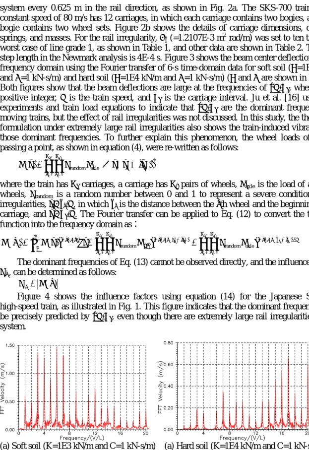
system every 0.625 m in the rail direction, as shown in Fig. 2a. The SKS-700 train with a constant speed of 80 m/s has 12 carriages, in which each carriage contains two bogies, and each bogie contains two wheel sets. Figure 2b shows the details of carriage dimensions, dampers, springs, and masses. For the rail irregularity, Ar (=1.2107E-3 m2 rad/m) was set to ten times the worst case of line grade 1, as shown in Table 1, and other data are shown in Table 2. The time step length in the Newmark analysis is 4E-4 s. Figure 3 shows the beam center deflections in the frequency domain using the Fourier transfer of 6-s time-domain data for soft soil (K=1E3 kN/m and C=1 kN-s/m) and hard soil (K=1E4 kN/m and C=1 kN-s/m) (K and C are shown in Fig. 2a).
Both figures show that the beam deflections are large at the frequencies of nV/Lc, where n is a positive integer, V is the train speed, and Lc is the carriage interval. Ju et al. [16] used field experiments and train load equations to indicate that nV/Lc are the dominant frequencies of moving trains, but the effect of rail irregularities was not discussed. In this study, the theoretical formulation under extremely large rail irregularities also shows the train-induced vibration has those dominant frequencies. To further explain this phenomenon, the wheel loads of a train passing a point, as shown in equation (4), were re-written as follows:
( )
∑∑
= =−
−
= Nc w
1 j
N 1 k
c
k jt )
t t ( P R )
t (
P random axle δ (12)
where the train has Nc carriages, a carriage has Nw pairs of wheels, Paxle is the load of a pair of wheels, Rrandom is a random number between 0 and 1 to represent a severe condition of rail irregularities, tk=sk/V, in which sk is the distance between the kth wheel and the beginning of the carriage, and tc=Lc/V. The Fourier transfer can be applied to Eq. (12) to convert the trainload function into the frequency domain as:
∑∑
∫ ∑∑
= =
+
−
= =
+
∞ −
∞
−
− = =
= c w k c Nc w k
1 j
N 1 k
V / ) jL s ( f 2 i N
1 j
N 1 k
) jt t ( f 2 i axle t
f 2
i dt R P e R P e
e ) t ( P )
f (
P π random π random axle π (13)
The dominant frequencies of Eq. (13) cannot be observed directly, and the influence factors, Rf , can be determined as follows:
) P( f
Rf = (14)
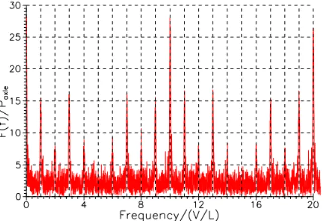
Figure 4 shows the influence factors using equation (14) for the Japanese SKS-700 high-speed train, as illustrated in Fig. 1. This figure indicates that the dominant frequencies can be precisely predicted by nV/Lc, even though there are extremely large rail irregularities in the system.
(a) Soft soil (K=1E3 kN/m and C=1 kN-s/m) (a) Hard soil (K=1E4 kN/m and C=1 kN-s/m) Fig. 3 Vertical-direction measured frequency-domain particle velocities at the beam center under
a train speed of 80 m/s
Fig. 4. Train load influence factors using Eq. (14) for the SKS-700 high-speed train 3. Finite element analyses and field measurements
Since Timosheko beam theory is not suitable to obtain the ground vibrations induced by moving trains, this section uses finite element analyses and field measurements to investigate their behavior. The finite element program can be found on the website (myweb.ncku.edu.tw/~juju).
3.1 Embankment dimensions and soil properties
The field measurements were performed in the center of Taiwan, as shown in Fig.5a, with the embankment dimensions shown in Fig. 5b. The rails are support on a concrete slab system, with a 19-cm-thick upper concrete bed for sustaining the rail, a 4.5-cm-thick cement-asphalt layer (CA layer) for cushioning, and a 33-cm-thick bottom concrete bed for sustaining the track structure on the soil foundation. The rail is the JIS-60-kg type supported on the upper concrete bed with a support interval of 0.625 m in the rail direction (X-direction). The Young’s modulus, Poisson’s ratio and mass density for the concrete bed are 2E7 kN/m2, 0.15, and 2.4 T/m3, while those for the cement-asphalt layer are 0.6E6 kN/m2, 0.25, and 1.6 T/m3, and those for the rail are 2E8 kN/m2, 0.3, and 7.85 T/m3, respectively. The soil profile contains 20-m compact sand, 10-m silty sand, and the rest is very hard sand. The Young's modulus of the surface soil is 4E5 kN/m2, and that of more than 50 m under the ground is 8E5 kN/m2. Linear interpolation was applied to determine it between these two depths. The mass density and Poisson’s ratio of the soil are 2 t/m3 and 0.49, respectively. Rayleigh damping was use in this study. The two factors of α and β in ([Damping]=α[Mass]+β[Stiffness]) for the soil equal 0.774/s and 3.73×10⁻⁴ s, respectively, which gives an approximately 2% damping ratio at a frequency of 4 Hz and 15 Hz. These material properties were estimated according to the soil investigations near our experiment location when the Taiwan high-speed rail was built, and the soil investigation data can be found on-line (www.moeacgs.gov.tw/main.jsp).
Length unit : cm
242 700
143.5 222
19 4.5 33
225 225
CA layer Rail
(a) Experiment location in the center of Taiwan (b) Embankment and railway dimensions Fig. 5 Illustration of the embankment and railway for numerical and experimental analyses
M1=38.9 T Ix1=97.2 T-M Iy1=1470 T-M Iz1=1267.5 T-M
1303
1301,1302
M3=1.77 T Ix3=0.71 T-M Iy3=0.18 T-M Iz3=0.71 T-M 1201~1204
1~4 101~104
401 404
501 504 603 604 601
604
~201
204
801~804 701~704
1101~1102 1103~1104
cx1,cy1,cz1
kx1,ky1,kz1
cz2
kz2
master node node (slave node) spring and damper
moving wheel element
2m0.29m0.28m0.43m
M2,Ix2, Iy2,Iz1
cx4,kx4 cy3=2.5 kN-s/m ky3=11000 kN/m
201 601,602 202
1001
1003
1201 1202
301 302
401 1003
501 502
402 603,604
0.3m2.01m 1.44m
Railway carriage
901 902
25m cx5
cy5
cz5
kx5
ky5
2 2 2
~
301
304~ ~ ~
cz2=40 kN-s/m kz2=1200 kN/m cx1=2500 kN-s/m cy1=60 kN-s/m cz1=20 kN-s/m kx1=140 kN/m ky1=140 kN/m kz1=330 kN/m
2 2 2
~
M2=3 T Ix2 =2.47 T-M2 Iy2 =3.69 T-M2 Iz1 =3.05 T-M2 cx4 =2.5 kN-s/m kx4 =16000 kN/m cx5=2000 kN-s/m,cy5=25 kN-s/m,cz5=25 kN-s/m kx5=4000 kN/m,ky5=kz5=0 kN/m
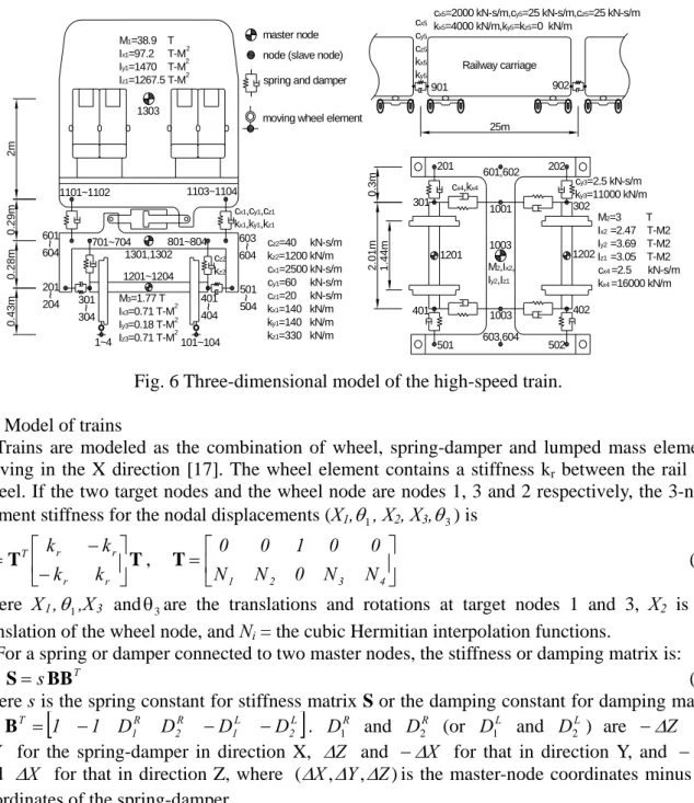
Fig. 6 Three-dimensional model of the high-speed train.
3.2 Model of trains
Trains are modeled as the combination of wheel, spring-damper and lumped mass elements moving in the X direction [17]. The wheel element contains a stiffness kr between the rail and wheel. If the two target nodes and the wheel node are nodes 1, 3 and 2 respectively, the 3-node element stiffness for the nodal displacements (X1,θ1, X2, X3,θ3) is
T T
S
−
= −
r r
r r
T
k k
k
k ,
=
4 3 2
1 N 0 N N
N
0 0 1 0
T 0 (15)
where X1,θ1,X3 andθ are the translations and rotations at target nodes 1 and 3, X3 2 is the translation of the wheel node, and Ni = the cubic Hermitian interpolation functions.
For a spring or damper connected to two master nodes, the stiffness or damping matrix is:
s BBT
S= (16)
where s is the spring constant for stiffness matrix S or the damping constant for damping matrix
S, [ 2L]
L 1 R 2 R 1
T = 1 −1 D D −D −D
B . D1R and D2R (or D1L and D2L) are −∆Z and
∆Y for the spring-damper in direction X, ∆Z and −∆X for that in direction Y, and −∆Y and ∆X for that in direction Z, where (∆X,∆Y,∆Z)is the master-node coordinates minus the coordinates of the spring-damper.
Figure 6 shows the 3D model of the SKS-700 high-speed train, which contains spring-dampers, rigid bodies and lumped mass. These components can be appropriately simulated using the above wheel and spring-damper elements.
C A la ye r
X,Y,Z-sp ring s b e twe e n ra il a nd p la te e ve ry 0 .625 m in ra il d ire c tio n
Soil
C o nc re te p la te s
(a) Mesh near the railway
(b) 3D mesh
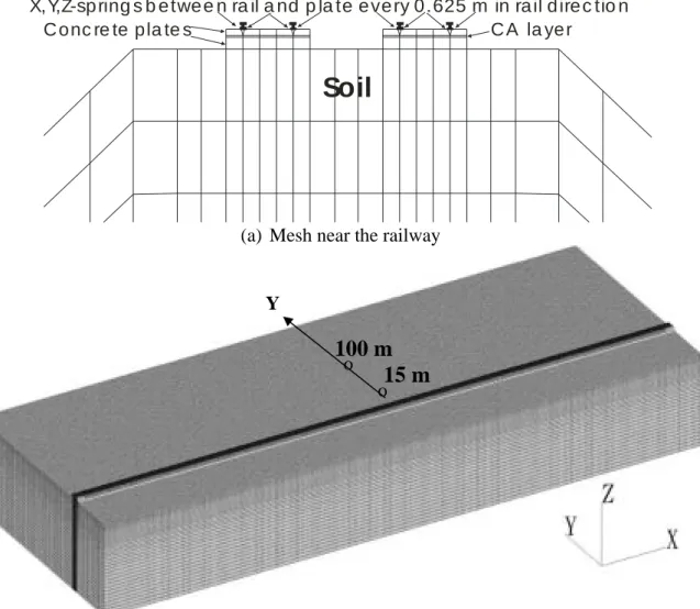
Fig. 7 A typical finite element mesh 3.3 Finite element model
The Newmark direct integration method and the consistent mass scheme were used to solve this problem with the solution scheme of the SSOR (Symmetric Successive Over-Relaxation) preconditioned conjugated gradient method [18]. The finite element model is 985 m long, 360 m wide and 150 m deep with the maximum solid element size of 2.5 m. The major part of the mesh is modeled by eight-node 3D solid elements for the soil and rail foundation. Rails are modeled by two-node 3D beam elements connected to the eight-node solid elements every 0.625 m in the X-direction using two spring elements (spring constant = 2.5E5 kN/m), and the nodes along the rails are the wheel target nodes of the train model. Finally, the five surfaces, except for the top surface of the mesh, are modeled by the absorbing boundary condition [19]. Figure 7 shows a typical 3D finite element mesh, which contains 9,861,576 degrees of freedom. The time step length is 0.005 seconds, and 3,000 time steps are simulated.
3.4 Comparisons between FEA and the field experiments
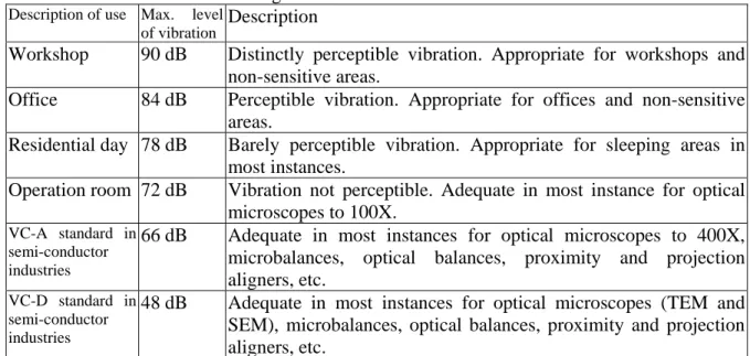
Analyzing vibrations using the 1/3 octave band in the frequency domain has become an international standard in the semi-conductor industry. Thus, this method, presented in decibels
Y
o
o 15 m 100 m
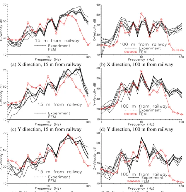
(dB) is utilized. Table 3 briefly presents the recommended vibration guidelines [20], and the calculation procedures can be found in [17]. In field experiments, there are two measurement stations with the distances of 15 and 100 m, respectively, from the railroad centerline (Fig. 7b), and each station had three velocity sensors set up to measure the X, Y, and Z vibration velocities, with 512 measurements per second. Figure 8 shows the experimental and finite element results at the locations of 15-m and 100-m stations under a train speed of 290 km/h. This figure indicates that the accuracy of the finite element analysis is acceptable, especially since the finite element results with variable frequencies agree well with the field experiments. The peaks of the vibration curves in these figures are caused by the dominant frequencies (nV/Lc).
Table 3. Recommended vibration guidelines
Description of use Max. level
of vibration Description
Workshop 90 dB Distinctly perceptible vibration. Appropriate for workshops and non-sensitive areas.
Office 84 dB Perceptible vibration. Appropriate for offices and non-sensitive areas.
Residential day 78 dB Barely perceptible vibration. Appropriate for sleeping areas in most instances.
Operation room 72 dB Vibration not perceptible. Adequate in most instance for optical microscopes to 100X.
VC-A standard in semi-conductor industries
66 dB Adequate in most instances for optical microscopes to 400X, microbalances, optical balances, proximity and projection aligners, etc.
VC-D standard in semi-conductor industries
48 dB Adequate in most instances for optical microscopes (TEM and SEM), microbalances, optical balances, proximity and projection aligners, etc.
To further validate the dominant frequencies of nV/Lc, all the three-direction particle velocities of the seven field measurements at the 100-m station were transformed to the frequency domain using the fast Fourier transform (FFT). The train velocities were measured between two locations divided by the difference in the arrival times, and we also used the tenth dominant frequency (f10) to calibrate the train speed (V=Lcf10/10=2.5f10 m/s, where Lc=carriage interval=25 m). Figure 9 shows the frequency-domain results, which were averaged from the seven experimental measurements in the three directions. This figure, directly obtained from experiments, indicates that the particle velocities are large at the frequencies of nV/Lc, even though the experiment location is 100 m away from the moving train.
(a) X direction, 15 m from railway (b) X direction, 100 m from railway
(c) Y direction, 15 m from railway (d) Y direction, 100 m from railway
(e) Z direction, 15 m from railway (f) Z direction, 100 m from railway
Fig. 8 Frequency-domain velocity at 15 and 100 m from the railroad centerline at a train speed of 290 km/h. (EXP = seven field experiments, FEM = finite element method).
Fig. 9 Average frequency-domain particle velocity of seven field measurements in the X, Y and Z directions at the 100-m station (Each data point is averaged from 21 values.)
3.5 Rail irregularities and layered soil effects for train speed under the soil Rayleigh speed
Since it is not easy to perform a parametric study for the effects of rail irregularities and layered soils using field experiments, we use finite element analyses to investigate these conditions. Five cases were analyzed, as follows: (1) a perfectly smooth rail (no rail irregularity), (2) the same case of Section 3.4 that the rail is in very good smooth, (3) the line grade 3 of rail irregularity, as shown in Table 1, (4) the line grade 1 of rail irregularity, as shown in Table 1, when the rail is very rough, and (5) homogeneous soil with the soil Young’s modulus of 5E5 kN/m2. In addition, the same soil as in section 3.4 and the rail irregularity data of Table 2 were used. Figure 10 shows the surface displacements of finite element analyses for cases 1 to 3, and Fig. 11 shows the finite element results, which indicate the following features:
(1) The train–induced ground vibration is extremely small when the rail is perfectly smooth;
however, for case 1 with a minor rail irregularity under the coefficient (Ar) smaller than the line grade 6 (very good condition), the train-induced ground vibration is significantly increased. At 200 m from the railway, the ground vibration of case 1 is an averagely 24 dB larger than that for the case with no rail irregularity, which means that the actual ground vibration is 16 times bigger. Thus, train-induced ground vibrations are significant due to the rail unevenness.
(2) As shown in Fig. 10a for the perfectly smooth rail the train-induced ground vibration is like the displacements compressed by the point loads of the train wheels moving in the railway direction. This type of problem can be solved by the theoretical steady-state solution in the reference [21], and the result is similar to that in Fig.10a. For a subsonic moving load on a half-infinite soil, the displacement decay is approximately in the order of r [22], where r is the distance between the displacement and point load. While the steady-state displacement under a series of moving loads may be more complicated, the displacement decay is still fast from the finite element as well as theoretical solutions [21]. For example, for the ground vibrations at the 15-m station, the 3.2-Hz vibration is still similar for cases 1 and 2, but very different at the 100-m station, which means that the vibration decay is much larger for the perfectly smooth case.
(3) Figure 11 shows that the ground vibrations at the 15-m station are similar for cases 2 (layered soil) and 5 (homogeneous soil), but those at 200-m are significantly different, which means that the vibrations decay fast with homogeneous soils. The reason is because the parts of vibrations at the layered soil will be reflected back and this condition, named the love wave, means that the vibrations will not decay easily along the soil surface. The love wave is mainly for the wave propagation of the transverse shear along the soil surface. Thus, Fig.11 shows that the Z-ground vibrations decay slower than those in the X and Y directions.
(4) Even though the phenomenon of train-induced ground vibrations is complicated, we can conclude it as follows using the basic theory of wave: The rail irregularities are the major source to induce ground vibrations when trains move on embankments. For the case of a perfectly smooth rail, the ground vibrations decay fast, but for vibrations induced by rail irregularities, the major part of the vibrations propagates in the form of a Raleigh wave which is not easy to decay on the soil surface. If the soil profile is layered, the vibration reflected between soil layers will further cause a slow decay of the train-induced ground vibrations.
(a) Case 1: No rail irregularity
(b) Case 2: Ar=2.5E-6 m2 rad/m<Ar of line-grade-6 (very good case)
(c) Case 3: Ar of line-grade-3 (poor case)
Fig.10 Soil surface displacements for the train speed of 290 km/h (Displacements are magnified by 3E6 times).
(a) X direction, 15 m from railway (b) X direction, 100 m from railway
(c) Y direction, 15 m from railway (d) Y direction, 100 m from railway
(e) Z direction, 15 m from railway (f) Z direction, 100 m from railway
Fig.11 Frequency-domain velocity at 15 and 100 m from the railroad centerline at a train speed of 290 km/h from five finite element analyses of section 3.5 (Case1: Ar=0, Case 2:
Ar=2.5E-6 m.rad, Case 3: Ar=Line grade 3, Case 4: Ar=Line grade 1, and Case 5:
Ar=2.5E-6 m.rad and homogeneous soil)
4. Train speed over soil Rayleigh speed with rail irregularity effect
Finite element analyses performed by Ju and Lin [21] indicated that ground vibrations increase considerably and decay slowly when the train speed exceeds the soil Rayleigh speed (supersonic train speed). However, rail irregularities were not considered in their analyses. In this section, the effect of rail irregularities will be discussed when the train speed exceeds the soil Rayleigh speed. The soil is set to homogeneous with the Young’s modulus of 1E5 kN/m2, Poisson’s ratio of 0.48, and mass density of 2 T/m2, so the soil Rayleigh speed is 445 km/h.
There are six cases with two train speeds of 500 and 600 km/h, and three rail irregularity coefficient Ar of 0 (perfectly smooth), 2.5E-6 (very good smoothness), and 68.16E-6 rad.m2/m (line grade 3 and poor smoothness). Other data and dimensions are the same as those in section 3.3. Figure 12 shows the surface displacements of finite element analyses for Ar of 0 and 68.16E-6 rad.m2/m under the train speed of 500 km/h, and Figs. 13 and 14 shows the finite element results, which indicate the following features:
(1) The vibration pattern is difficult to damp and is like the displacement compressed by the trainloads moving in the railway direction. Notably, the vibration at the first dominant frequency (V/Lc) is much higher than those of other frequencies. The reason is because the vibration decay is very slow when the train speed is faster than the soil Rayleigh speed, and the vibration of the first dominant frequency having the longest wave length is even more difficult to damp.
(2) The ground vibrations with or without rail irregularities are not very different, and the cases with rail irregularities are only larger at high-frequency vibrations. When train-induced vibrations move away from the railway, the high-frequency vibrations will be damped fast, and the vibration at the first dominant frequency will be the most obvious, which means that the effect of rail irregularities is minor for train speeds over the soil Rayleigh speed. The train-induced vibrations under a very poor rail irregularity can be still dominant, but such a poor rail irregularity is almost impossible for the high-speed rail system.
(3) The vibrations in the vertical (Z) direction are obviously much larger than those in the other two directions, but this condition was not found for the train speed smaller than the soil Rayleigh speed (subsonic train speeds). This is because the rail irregularities are the major sources to produce ground vibrations for subsonic train speeds, and the vertical and transverse rail irregularities are often in a similar range (the same in this study), which causes similar vibration magnitudes in all three directions. However, for supersonic train speeds, the most important vibration source is the vertical trainload, so the largest vibration should be in that direction.
5. Conclusions
In this study, a 2D train-rail interaction solution of the Timosheko beam was used to investigate the characteristics of train-induced vibration. The results indicate that the train-induced vibrations are large at the dominant frequencies of nV/Lc, even though the rail is very rough, where n is a positive integer, V is the train speed, and Lc is the carriage interval.
Moreover, the theoretical formulation of train wheel loads under extremely large random rail irregularities also shows that the loads have those dominant frequencies.
This study indicates that train-induced ground vibrations are mainly due to the rail unevenness for subsonic train speeds. When the rail is perfectly smooth, the train–induced ground vibration is extremely small, but with a minor rail irregularity, the train-induced ground vibration can be significantly increased. This is because the train-induced vibrations without rail
irregularities decay very fast, while those induced from the rail irregularities propagate in the form of a Raleigh wave that is not easy to decay on the soil surface. In addition, if the soil profile is layered, the vibration reflected between soil layers will further cause a slow decay of the train-induced ground vibrations. However, for trains moving on bridges, the major vibration may not be generated from rail irregularities, since the resonance of the train’s dominant and bridge’s natural frequencies can be the most important source of ground vibrations.
On the other hand, for supersonic train speeds, the ground vibrations with or without rail irregularities are not very different. The reason is because the vibration decay is very slow, and since the vibration of the first dominant frequency has the longest wave length, it is even more difficult to damp, so other vibrations are not obvious. Thus the effect of rail irregularities is minor for train speeds over the soil Rayleigh speed.
(a) No rail irregularity
(b) Ar of line-grade-3 (poor case)
Fig.12 Soil surface displacements for the train speed of 600 km/h (Displacements are magnified by 5E5 times).
(a) X direction, 15 m from railway (b) X direction, 100 m from railway
(c) Y direction, 15 m from railway (d) Y direction, 100 m from railway
(e) Z direction, 15 m from railway (f) Z direction, 100 m from railway
Fig.13 Frequency-domain velocity at 15 and 100 m from the railroad centerline at supersonic train speeds of 500 km/h
(a) Z direction, 15 m from railway (b) Z direction, 100 m from railway
Fig.14 Frequency-domain velocity in the Z direction at 15 and 100 m from the railroad centerline at supersonic train speeds of 600 km/h
References
[1] P. Remington, J. Webb, Estimation of Wheel/Rail Interaction Forces in the Contact Area due to Roughness, Journal of Sound and Vibration 193 (1) (1996) 83-102.
[2] T.X. Wu, D.J. Thompson, Vibration Analysis of Railway Track with Multiple Wheels on the Rail, Journal of Sound and Vibration 293 (1) (2001) 69-97.
[3] Y. Suda, T. Miyamoto, N. Katoh, Active Controlled Rail Vehicles for Improved Curving Performance and Response to Track Irregularity, Vehicle System Dynamics 35 (2001) 23-40.
[4] Y.S. Wu, Y.B. Yang, J.D. Yau, Three-Dimensional Analysis of Train-Rail-Bridge Interaction Problems, Vehicle System Dynamics 36 (1) (2001) 1-35.
[5] F.T.K. Au, J.J. Wang, Y.K. Cheung, Impact Study of Cable-Stayed Railway Bridges with Random Rail Irregularities, Engineering Structures 24 (5) (2002) 529-541.
[6] Y.S. Wu, Y.B. Yang, Steady-State Response and Riding Comfort of Trains Moving over a Series of Simply Supported Bridges, Engineering Structures 25 (2) (2003) 251-265.
[7] T.X. Wu, D.J. Thompson, On The Parametric Excitation of The Wheel/Track System, Journal of Sound and Vibration 278 (4-5) (2004) 725-747.
[8] Z.F. Wen, X.S. Jin, Effect of Track Lateral Geometry Defects on Corrugations of Curved Rails, Wear 259 (2005) 1324-1331.
[9] M.H. Kargarnovin, D. Younesian, D. Thompson, C. Jones, Ride Comfort of High-Speed Trains Travelling Over Railway Bridges, Vehicle System Dynamics 43 (3) (2005) 173-197.
[10] A. Johansson, C. Andersson, Out-of-Round Railway Wheels - a Study of Wheel Polygonalization Through Simulation Of Three-Dimensional Wheel-Rail Interaction and Wear, Vehicle System Dynamics 43 (8) (2005) 539-559.
[11] Y.T. Fan, W.F. Wu, Dynamic Analysis and Ride Quality Evaluation of Railway Vehicles - Numerical Simulation and Field Test Verification, Journal of Mechanics 22 (1) (2006) 1-11.
[12] J.A. Forrest, H.E.M. Hunt, Ground Vibration Generated by Trains in Underground Tunnels, Journal of Sound and Vibration 294 (4-5) (2006).
[13] X. Sheng, M. Li, C.J.C. Jones, D.J. Thompson, Using the Fourier-Series Approach to Study Interactions between Moving Wheels and a Periodically Supported Rail, Journal of Sound and Vibration 303 (3-5) (2007) 873-894.
[14] L. Fryba, Vibration of Solids and Structures under Moving Load, Thomas Telford, London,
1999.
[15] X. Lei, N.A. Noda, Analyses of Dynamic Response of Vehicle and Track Coupling System with Random Irregularity of Track Vertical Profile, Journal of Sound and Vibration 258 (1) (2002) 147-165.
[16] S.H. Ju, H.T. Lin, Jeng-Yuan Huang, Dominant Frequencies of Train-Induced Vibrations, Journal of Sound and Vibration 319 (2009) 247-259.
[17] S.H. Ju, H.T. Lin, Experimentally Investigating Finite Element Accuracy for Ground Vibrations Induced by High-Speed Trains, Engineering Structures 30 (3) (2007) 733-746.
[18] S.H. Ju, K.S. Kung, Mass Types, Element Orders and Solving Schemes for the Richards Equation, Computers & Geosciences 23 (1997) 175-187.
[19] S.H. Ju, Y.M. Wang, Time-Dependent Absorbing Boundary Conditions for Elastic Wave Propagation, International Journal for Numerical Method in Engineering 50 (2001) 2159-2174.
[20] C.G. Gordon, Generic Criteria for Vibration Sensitive Equipment, Optics and Metrology 1619 (1991) 71-75.
[21] S.H. Ju, H.T. Lin, Analysis of Train-Induced Vibrations and Vibration Reduction Schemes above and Below Critical Rayleigh Speeds by Finite Element Method, Soil Dynamic and Earthquake Engineering 24 (12) (2004) 993-1002.
[22] G. Lykotrafitis, H.G. Georgiadis, The Three-Dimensional Steady-State Thermo-Elastodynamic Problem of Moving Sources over a Half Space, International Journal of Solids and Structu
![Table 1. Rail irregularity classification [15]](https://thumb-ap.123doks.com/thumbv2/9libinfo/9190566.470841/3.892.98.776.379.961/table-rail-irregularity-classification.webp)