車輛行車在軌道損壞與地震作用下之振動特性與安全分析

1. Introduction

High-speed trains have become one of the most important forms of transportation in many countries. Thus, the safety of moving high-speed trains during an earthquake is a subject of great concern in railway engineering. Investigations of the dynamic interaction of trains and railway structures have been developed by many authors; however, to date rather limited efforts have been devoted to examining the seismic resistance of high-speed trains. In order to estimate the related behavior and risks, Yang and Wu [1] used 3-D train and bridge models to investigate the stability of trains initially resting on or travelling over bridges under different seismic excitations, with the effects of the track system taken into account. Xiu Luo [2] evaluated the dynamic response behavior of railway vehicles with a simplified analytical model and proposed a code-type provision based on the concept of energy balance, in which the spectral intensity (SI) is employed as an index for assessment in their paper. Tanabe et al.

[3] used a finite element method to solve the dynamic interaction of a high-speed train and railway structure during an earthquake. A substructure model was devised to obtain the approximated combined motion of a long train with many cars and the railway structure during an earthquake. Fryba and Yau [4, 5] analyzed the vibration of suspended bridges subjected to the simultaneous action of moving loads and vertical support motions due to an earthquake, and their results indicate that the interaction of both the moving and seismic forces may substantially amplify the response of long-span suspended bridges in the vicinity of the supports and increase with the rising speed of trains. Xia et al. [6] investigated a train traveling over a continuous seven-span viaduct shaken by an earthquake, and showed that lack of considering seismic traveling wave effect might lead the train manipulation to an unsafe conclusion.

Obviously, to simulate the dynamic behaviors of a high-speed train is complicated due to the interaction between the train and the railway structure, especially during earthquakes.

However, for the sake of safety assessment, we study the risk of train derailment by using a three-dimensional (3D) time-domain finite element method. To the best knowledge of the authors, this type of finite element analysis is both complex and rare in the literature. Based on the situation of soil-rail-train interaction under seismic excitation, a dynamic response behavior of the train system modelled by FEM, including both the absorbing boundary condition and rail irregularity, has been simulated. Some new results found in these numerical analyses clearly explain the behaviors of trains moving on embankments during seismic loads. This paper also shows how to generate the finite element procedures and examines the derailment of the train during severe earthquake.

2. Models of train, rail irregularity and derailment 2.1 Train model

We set the rail direction in the X axis, the earthquake direction in the Y axis, and the negative gravity direction in the Z axis. Moving trains are modeled as a combination of moving wheel elements, spring-damper elements, lumped mass, and rigid links. The wheel element contains a stiffness k

between the rail and wheel in the X, Y, or Z direction [7]. If the two target nodes and the wheel node are nodes 1, 3, and 2 respectively, the three-node element stiffness for the nodal displacements (X

, θ , X

, X

, θ ) is:

T T

S 



 





−

= −

r r

r T r

k k

k

k ,



 



=

4 3 2

1 0

0 0 1 0 0

N N N

T N

(1)

where X

, θ

^,X

^{, and} θ

are the translations and rotations at target nodes 1 and 3, respectively,

X

is the translation of the wheel node, and N

represents the cubic Hermitian interpolation

functions. The trainload F on the wheel is in equilibrium with the system, so this load F on

node 2 should be transformed into nodes 1 and 3 to obtain the force vector f as follows:

] [ N

N

0 N

N

F

T

=

f (2)

For rail irregularities, the forces (f

) need to be added to the global forces, as follows:

) ( ]

[ N

N

1 N

N

k

r

X

T

r

= −

f (3)

where r

(X) is a function of the rail irregularity, and X is the wheel location in the X axis. For a spring or damper connected to two master nodes, the stiffness or damping matrix is:

sBB

S = (4)

where s is the spring constant for stiffness matrix S or the damping constant for damping matrix S, and B

= [ 1 − 1 D

D

− D

− D

] . D

and D

(or D

and D

) are − Δ Z and Δ Y for the spring-damper in direction X, Δ Z ^and − Δ ^X for that in direction Y, and − Δ Y and X Δ for that in direction Z, where ( Δ X , Δ Y , Δ Z ) ^{are the} master-node coordinates minus the coordinates of the spring-damper. If there is no master node connected to the spring-damper, Δ X , Δ Y , ^and Δ Z are zero. In this study, each master node can contain three mass values and three moment of inertia values.

Figure 1 shows the 3D model of the SKS-700 high-speed train, which contains spring-dampers, rigid bodies and lumped masses. These components can be appropriately simulated using the above wheel and spring-damper elements.

2.2 Rail irregularity

A function r

( X ) of the rail irregularity [8] was used in this study.





+

= +

=

k

k k k

N k

k k k

v

X a X a Vt

r

1 1

) cos(

) cos(

)

( ω φ ω φ ⁽⁵⁾

where a is the amplitude,

ω

is a frequency (rad/m) within the upper and lower limits of the frequency [ ω

^, ω

^], φ

is a random phase angle in the interval [0,

], X is the global coordinate in the rail direction, V is train speed, t is time, and N is the total number of terms.

The parameters a and

ω

are computed by:

ω Δ ω ⁾ ( 2

k

G

a = , ω

= ω

+ ⁽ k − ^{1 / 2 )} Δ ω , and Δ ω = ( ω

− ω

) / N , k=1,2,…,N (6)

) (

) ) (

(

2 2 4

2 1 2 2 2

ω ω ω

ω ω ω ω

+

=

+

rr

G A (7)

Where

ω

is the power spectral density function, A

is the irregularity coefficient, and ω

^and ω

are frequencies to change the shape of

ω

. In this paper, we will perform field measurement and finite element analysis of high-speed trains running in Taiwan. The rail irregularity has the amplitude of about 2 mm per 20 m of the rail. We used the irregularity parameters as shown in Table 1, and Fig. 2 shows the profile.

Table 1. Rail irregularity parameters used in the numerical analyses A

(m

rad/m) ω

^(rad/m) ω

^(rad/m) ω

^(rad/m) ω

^(rad/m) N

0.025E-4 0.0233 0.131 0.2 20 2000

2.3 Train derailment

The maximum wheel derailment coefficient (Q/P) from all the wheelsets of a train is

calculated as follows [9] (Jun and Qingyuan, 2005):

Q/P=Max(Q

/P

), i=1,n (8) where Q

and P

are the horizontal and vertical forces of the i

wheelset, and n means the total

number of wheelsets for the train.

The specification standards for derailment prevention in various countries are: (1) Western Europe: Q/P<0.8, where the average movement distance of Q/P is set to 2m, (2) Japan: Q/P< 0.8, where the continuous action time of Q/P is less than 0.015 s, (3) North America: Q/P<1.0, and (4) China: Q/P<1.0 (allowable limit), 1.2 (danger limit). In this study, the Western Europe an standard was used, since the finite element analysis requires a specific average movement distance or time interval to calculate the train derailment coefficient.

3. Illustration of seismic loading and embankment dimensions 3.1 Illustration of earthquakes used in this study

The characteristics of an earthquake include its magnitude and frequency ranges. In this study, the maximum earthquake magnitude was set to 0.25 g, and three frequency ranges were used for different region zones in Taipei, Taiwan using the software Simqke [10]. Case 1 is the region with soft soil, so the frequencies of the seismic loading are dominated at the low frequency range. Case 2 is the region with moderately hard soil for higher frequency earthquakes. We also generated an earthquake for Case 3 that has very high frequency loading. Figures 3 and 4 show the earthquake accelerations in the time and frequency domains, respectively. The difference among the three earthquakes can be clearly seen from the frequency domain (Fig. 4).

3.2 Absorbing boundary conditions

In this paper, the absorbing boundary condition of equation (9) was used along the finite element boundaries to avoid fake wave reflection.

0 x )u

t c

(

1

i

=

∂

− ∂

∂

∂ for i=1,2 and 3. (9)

where x

is the positive local direction points into the domain, u

denotes the x

-displacement, and c

is the i-direction velocity divided by the cosine of the incidence angle. Ju and Wang [11]

(2000) evaluated time-dependent c

as:



 





∂

∂

∂

 ∂



 





∂

∂

∂

=





=

=

N 1

k 1

ik 1 N ik

1 k

ik ik

i x

u x u t

u t

c u

for i=1,2 and 3 (10)

where N is the number of nodes to obtain the average c

. Then, the forward Euler method derived from equation (9) is

1 n i, i n i, 1 n

i, x

Δtc u u

u ∂

+ ∂

+ =

(11)

where u

is the i-direction displacement at the current time step, u

is the i-direction displacement at the last time step, and Δ t is the time step length. In equation (11), all the values on the right side are known, so the current controlled displacements are obtained.

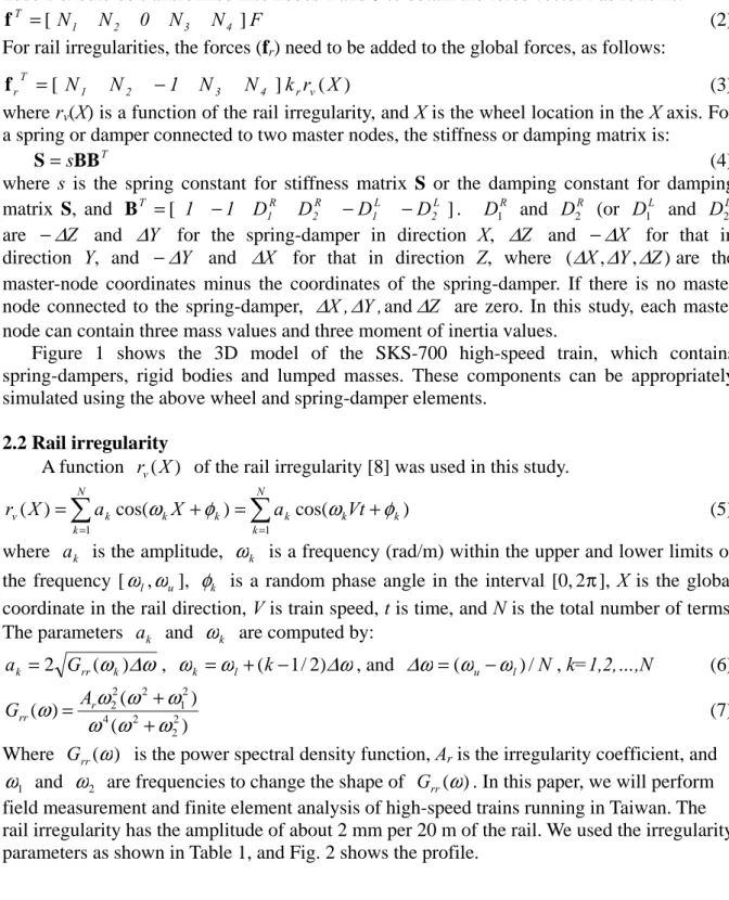
3.3 Embankment dimensions and soil properties

The paper studied the behavior of trains moving on embankments, as shown in Fig. 5,

under seismic loading. The rails are supported on a concrete slab system, with a 19-cm-thick

upper concrete bed for sustaining the rail, a 4.5-cm-thick cement-asphalt layer (CA layer)

for cushioning, and a 33-cm-thick bottom concrete bed for sustaining the track structure on

the soil foundation. The rail is the JIS-60-kg type supported on the upper concrete bed with

a support interval of 0.625 m in the rail direction (X-direction). The Young’s modulus,

Poisson’s ratio and mass density for the concrete bed are 2E7 kN/m

, 0.15, and 2.4 T/m

,

while those for the cement-asphalt layer are 0.6E6 kN/m

, 0.25, and 1.6 T/m

, and those for the rail are 2E8 kN/m

, 0.3, and 7.85 T/m

, respectively. The Young's modulus of the surface soil is 4E5 kN/m

, and that of more than 50 m under the ground is 0.8E5 kN/m

. Linear interpolation was applied to determine it between these two depths. The mass density and Poisson’s ratio of the soil are 2 t/m

and 0.49, respectively. Rayleigh damping was used in this study. The two factors of α and β in ([Damping]=α[Mass]+β[Stiffness]) for the soil equal 0.774/s and 3.73 ×10

s, respectively, which gives an approximately 2% damping ratio at a frequency of 4 Hz and 15 Hz.

4. Time-domain finite element model with the seismic loading

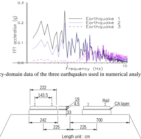
The Newmark direct integration method and the consistent mass scheme were used to solve this problem in the time domain with the solution scheme of the SSOR (Symmetric Successive Over-Relaxation) preconditioned conjugated gradient method [12]. The major advantage of the above scheme is that the computer memory requirement can be minimized, and the numerical solution can be efficient. The finite element model is 2,145 m long, 235 m wide and 97 m deep with the maximum solid element size of 2.5 m. The major part of the mesh is modeled by eight-node 3D solid elements for the soil and rail foundation including CA layers and concrete beds. Rails are modeled by two-node 3D beam elements connected to the eight-node solid elements every 0.625 m in the X-direction using two groups of three spring elements (spring constant = 2.5E5 kN/m) in the global X,Y and Z directions, and the nodes along the top of the rails are the wheel target nodes of the train model.

For the boundary condition of the mesh, the four surfaces, except for the top and bottom surfaces of the mesh, are modeled by the absorbing boundary condition [11], so that the vibration passing these mesh boundaries will not be reflected. Along the soil surface, all the nodes are free to move, and along the bottom of the mesh, the vertical degrees of freedom of all the nodes are fixed. The time-history of the earthquake accelerations, as shown in Fig. 3, then were integrated to obtain the nodal displacements. These nodal displacements were applied to the nodes in the Y direction along the mesh bottom, which means that an earthquake is applied to the problem domain in the Y direction. In practice, the phenomenon is complicated, since the earthquake displacement on the bottom of the mesh can be irregular.

To simplify the finite element analyses, we used a uniform distribution of earthquake displacements along the bottom of the mesh in this study. Figure 6 shows a typical 3D finite element mesh, which contains 12,975,036 degrees of freedom, and more details about mesh near the railway are specified in Fig. 6 (a). The time step length is 0.005 seconds, and 4,000 time steps are simulated. For this analysis, the computer memory requirement is about 6.5 GB, and the computer time requirement is nine days using an Intel I7-950 personal computer.

The finite element result of the train-induced ground vibration with rail irregularities has been validated using field experiments in the reference [13].

5. Investigation of train derailment 5.1 Train speed and rail irregularity effects

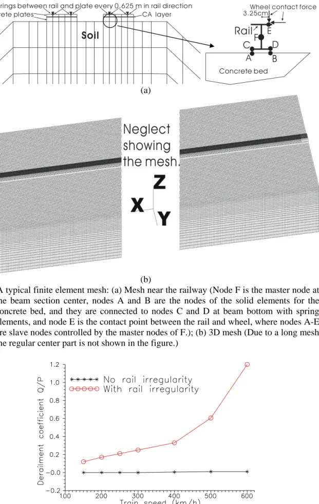
The maximum derailment coefficients versus train speeds with or without rail irregularities are determined in this section. These values were obtained from the maximum derailment coefficients of all train wheelsets and the time interval required for the train to pass through the finite element domain of 2000 m. Seven different train speeds from 150 to 600 km/h were studied with the perfectly smooth rail and the rail irregularities, as shown in Table 1. The maximum derailment coefficients calculated from finite element results are shown in Fig. 7, which indicates the following features:

(1) For the case of a perfectly smooth rail, the derailment coefficients of train wheelsets are

near zero, and they are almost independent of train speeds. It is noted that the soil

Rayleigh speed of this test location is about 850 km/h, so all the conclusions of this study do not consider a supersonic train speed. This result is reasonable, since the vibration of a moving train should be considerably small for a rail without roughness; however, a perfectly smooth rail is not possible in practice.

(2) With the minor rail irregularities in Table 1, the derailment coefficients of train wheelsets are highly dependent on train speeds, and faster trains will cause larger derailment coefficients. The coefficient gradually approaches zero for the train speed close to zero, and it seems that the coefficient increases with train speed with more than a linear relationship. This condition can be explained from equation (5). For a certain constant irregularity frequency ( ω

= ω

V =constant), the increase of V will decrease ω

, and also cause a larger a

from equation (6). This, therefore, produces a larger rail irregularity (r

(X)), and the value is approximately proportional to V

if we set ω

= ω

= ω

= ω

/ V in equation (7).

(3) From the above discussions, one obtains that the rail should be as smooth as possible in order to decrease the derailment of moving trains. For a faster train, the train derailment will be larger, which is due to the rail irregularities. Since it is impossible to avoid rail irregularities completely, the train speed should thus be limited due to safety.

5.2 Earthquake effect

5.2.1 Derailment due to earthquake types and magnitude

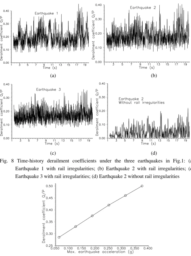
This section investigates the variation of the derailment coefficient due to different seismic loadings. A mentioned in section 3.2, three different earthquakes were analyzed, the train speed was set to 300 km/h, and the rail irregularities in Table 1 were used in finite element analyses. Figure 8 shows the maximum derailment coefficient of all the train wheelsets changing with time during the three earthquakes. To understand the combined effect of rail irregularities and seismic loading, Fig. 8d shows the results during earthquake 2 without rail irregularities. Thus, we can compare it with Fig. 8b that contains rail irregularities. Figure 9 shows the maximum derailment coefficient of all the train wheelsets when the train passes through the mesh domain of 2,000 m for the second earthquake (20-second seismic loading), while the acceleration of earthquake 2 (Fig. 3b) was multiplied by a factor from 0.25 to 1.5, so that the maximum acceleration of the earthquake is equivalent from 0.06 g to 0.375 g. The two figures indicate the following features:

(1) Figures 8b and 8c show that the rail irregularities contribute a lot of high frequency vibrations to the combined result for rail irregularities and seismic loading. The combined derailment coefficient of 0.41 is a little smaller than the sum of the two components from pure earthquake loading (0.22) and pure rail irregularities (0.25), which means that the combined effect of rail irregularities and seismic loading can not be ignored.

(2) Figure 8 indicates that the distributions of the derailment coefficients under the three earthquakes are similar, although the frequency distributions of the three earthquakes are very different (Fig. 3). However, the maximum derailment coefficients equal to 0.36, 0.41 and 0.45 under the three earthquakes in Fig. 8 are quite different, which is due the resonance of the train and earthquake. It can be seen in the frequency domain of Fig. 4 that the three earthquakes dominant frequencies are quite different. Obviously, the lowest-frequency earthquake causes the largest derailment coefficient, while the reverse is true for the highest-frequency earthquake. The first natural frequencies of the train carriage in the lateral and vertical directions are 0.6 and 0.5 Hz, respectively, which are in the low frequency range. Thus, the resonance between the train and earthquake increases the train vibration, which causes a larger derailment coefficient.

(3) The first natural frequencies of the train are often smaller than 1 Hz, which means that an

earthquake with dominant frequencies below 1 Hz may cause resonance between the moving train and seismic loading. A region with soft soil will usually cause the seismic loading to approach the low frequency range when an earthquake passes through. This condition makes the situation even worse, since the magnitude of seismic waves will be also enlarged when they pass through soft soil.

(4) If all the structural behaviors are linear elastic under a certain earthquake loading, the maximum derailment coefficients are quite linear in proportion to the magnitude of the earthquake, as shown in Fig. 9. When the earthquake is significantly small, the maximum derailment coefficients will be dominated by the rail irregularities, but the coefficients are gradually linear in proportion to the magnitude of earthquake when it increases. It is noted that this study only performed linear finite element analyses. For a large scale earthquake, the nonlinear behavior of rails and soils may produce a worse condition with regard to train derailment.

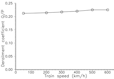
5.2.2 Derailment due to different train speeds under earthquake loading

The previous section indicated that a faster train has a larger derailment coefficient due to the effect of rail irregularities. This section investigates the relationship between train speeds and derailment coefficients under a certain seismic loading, in this case earthquake 2, as shown in Fig. 3b. Since the train derailment coefficient is highly dependent on the rail irregularities, they were not included in the finite element analysis. Thus, the behavior between train speeds and seismic loading can be easily recognized. Figure 10 shows the maximum derailment coefficient of all the train wheelsets when the train passes through the mesh domain of 2,000 m for the second earthquake (20-second seismic loading), while the train speed changed from 50 to 600 km/h. The figure indicates that the train derailment coefficient due to the seismic loading is almost independent of the train speed. Thus, one can analyze the train derailment coefficient under the seismic loading using a stopped train on the embankment, and this result can be applied to the train running with a certain speed. To consider the effect of rail irregularities, one can simply add the train derailment coefficients from the seismic loading and rail irregularities, and this value should be conservable.

6. Conclusions

(1) To simulate the derailment of trains moving on embankments under the seismic loading, the soil profile cannot be ignored. Generally, using the time-domain finite element method to simulate the 3D unbounded wave problem produces a large number of degrees of freedom.

Moreover, the wave will be reflected along the mesh boundary only if the traditional finite element method is used. However, this study overcame these obstacles in order to simulate the derailment of trains due to earthquakes. First, trains, including car bodies, bogies, wheel-axis sets, springs, and dampers, are modeled by assembling moving wheel elements, spring-damper elements, lumped masses, and rigid links. Then, a finite element mesh including rails, embankment foundation, and soil was generated using the traditional two-node beam elements and 3D 8-node isoparametric elements. For the boundary condition of the mesh, the four surfaces except for the top and bottom were modeled by the absorbing boundary condition to avoid fake wave reflection. Along the bottom of the mesh, the time-history of the earthquake displacements were applied to the nodes in the Y direction.

Using the above scheme, Newmark’s method can be used with the efficient solution scheme, the SSOR preconditioned conjugated gradient method, to perform the dynamic finite element analysis, which is exactly the same as the traditional time-domain finite element analysis.

(2) For the case of a perfectly smooth rail, the derailment coefficients of train wheelsets are

near zero, and they are almost independent of train speeds. However, with minor rail

irregularities, the derailment coefficients of train wheelsets are highly dependent on train speeds, and faster trains will cause larger derailment coefficients, and it thus seems that the coefficient increases with train speed in more than a linear relationship. Thus, to decrease the derailment of moving trains, the rail should be as smooth as possible. However since it is impossible to avoid rail irregularities completely, the train speed should be limitated due to safety.

(3) This study shows that the resonance between the train and earthquake plays an important role in train derailment. The first natural frequencies of the train are often smaller than 1 Hz, which means that an earthquake with dominant frequencies below 1 Hz may cause resonance between the moving train and seismic loading. Furthermore, the maximum derailment coefficients are relatively linear proportional to the magnitude of the earthquake, if the structural behaviors are not nonlinear.

(4) Without rail irregularities, the train derailment coefficient due to the seismic loading is almost independent of the train speed, but it is highly dependent on the train speed when rail irregularities are included. Moreover, the combined effect of rail irregularities and seismic loading can not be ignored, so to investigate train derailment under seismic loading without considering rail irregularities is of little practical use.

References

[1]. Y.B. Yang, Y.S. Wu, Dynamic stability of trains moving over bridges shaken by earthquakes, Journal of Sound and Vibration 258 (1) (2002) 65-94.

[2]. X. Luo, Study on methodology for running safety assessment of trains in seismic design of railway structures, Soil Dynamics and Earthquake Engineering 25 (2) (2005) 79-91.

[3]. M. Tanabe, N. Matsumoto, H. Wakui, M. Sogabe, H. Okuda,Y. Tanabe, A simple and efficient numerical method for dynamic interaction analysis of a high-speed train and railway structure during an earthquake, Journal of Computational and Nonlinear Dynamics, Transactions of the ASME 3 (4) (2008) 041002 (8 pages).

[4]. J.D. Yau, L. Fryba, Response of suspended beams due to moving loads and vertical seismic ground excitations, Engineering Structures 29 (12) (2007) 3255-3262.

[5]. L. Fryba, J.D. Yau, Suspended bridges subjected to moving loads and support motions due to earthquake, Journal of Sound and Vibration 319 (1-2) (2009) 218-227.

[6]. H. Xia, Y. Han, N Zhang, W.W. Guo, Dynamic analysis of train-bridge system subjected to non-uniform seismic excitations, Earthquake Engineering & Structure Dynamics 35 (2006) 1563-79.

[7]. S.H. Ju, H.T. Lin, Investigating vehicle dynamic response due to braking and acceleration, Journal of Sound and Vibration 303 (1-2) (2007) 46-57.

[8]. F. T. K. Au, J. J. Wang, Y. K. Cheung , Impact study of cable-stayed railway bridges with random rail irregularities, Engineering Structures 24 (5) (2002) 529-541.

[9]. X. Jun, Z. Qingyuan, A study on mechanical mechanism of train derailment and preventive measures for derailment, Vehicle System Dynamics 43 (2) (2005) 121-147.

[10]. D.A. Gasparini, E.H. Vanmarcke, Simulated earthquake motions compatible with prescribed response spectra. MIT civil engineering research report R76-4 (1976), Massachusetts Institute of Technology, Cambridge, MA.

[11]. S.H. Ju, Y.M. Wang, Time-dependent absorbing boundary conditions for elastic wave propagation, Int J Numer Method Eng 50 (2001) (9) 2159–2174.

[12]. S.H. Ju, K.J.S. Kung, Mass types, element orders and solution schemes for the Richards equation, Computers & Geosciences 23 (2) (1997) 175-187.

[13]. S.H. Ju, Investigation of train-induced ground vibrations using FEM and field

experiments, 4

International Symposium on Enviromental Vibration:prediction,

Monitoring and Evaluation, 2009.

M¹=38.9 T Ix1=97.2 T-M Iy1=1470 T-M I^z1=1267.5 T-M

1303

1301,1302

M3=1.77 T Ix3=0.71 T-M I^y3=0.18 T-M I^z3=0.71 T-M 1201~1204

1~4 101~104

401 404

501 504 603 604 601

604

~201

204

801~804 701~704

1101~1102 1103~1104

cx1,cy1,cz1

k^x1,k^y1,k^z1

c^z2 k^z2

master node node (slave node) spring and damper

moving wheel element

2m0.29m0.28m0.43m

M2,Ix2, I^y2,I^z1

c^x4,k^x4 cy3=2.5 kN-s/m ky3=11000 kN/m

201 601,602 202

1001

1201 1003 1202

301 302

401 1003

501 502

402

603,604 0.3m2.01m 1.44m

Railway carriage

901 902

25m cx5

cy5

c^z5 k^x5 ky5

2 2 2

~

301

304~ ~ ~

c^z2=40 kN-s/m k^z2=1200 kN/m cx1=2500 kN-s/m c^y1=60 kN-s/m c^z1=20 kN-s/m kx1=140 kN/m k^y1=140 kN/m k^z1=330 kN/m

2 2 2

~

M²=3 T Ix2 =2.47 T-M2 Iy2 =3.69 T-M2 I^z1 =3.05 T-M2 cx4 =2.5 kN-s/m kx4 =16000 kN/m cx5=2000 kN-s/m,cy5=25 kN-s/m,cz5=25 kN-s/m k^x5=4000 kN/m,k^y5=k^z5=0 kN/m

Fig. 1 Three-dimensional model of the high-speed train.

Fig. 2 Rail irregularity profile using the parameters in Table 1

(a) (b) (c)

Fig. 3 Time-history data of the three earthquakes used in numerical analyses: (a) Earthquake

1 (soft soil); (b) Earthquake 2 (moderate soil); (c) Earthquake 3 (hard soil)

Fig. 4 Frequency-domain data of the three earthquakes used in numerical analyses

Length unit : cm

242 700

143.5 222

19 4.5 33

225 225

CA layer Rail

Fig. 5 Illustration of the embankment and railway for finite element analyses

CA layer X,Y,Z-springs between rail and plate every 0.625 m in rail direction

Soil

Concrete plates

A

B

C D

3.25cm

Concrete bed

Wheel contact force

Rail

(a)

(b)

Fig. 6 A typical finite element mesh: (a) Mesh near the railway (Node F is the master node at

the beam section center, nodes A and B are the nodes of the solid elements for the

concrete bed, and they are connected to nodes C and D at beam bottom with spring

elements, and node E is the contact point between the rail and wheel, where nodes A-E

are slave nodes controlled by the master nodes of F.); (b) 3D mesh (Due to a long mesh,

the regular center part is not shown in the figure.)

Fig. 7 Derailment coefficient Q/P versus train speed with or without rail irregularities

(a) (b)

(c) (d)

Fig. 8 Time-history derailment coefficients under the three earthquakes in Fig.1: (a) Earthquake 1 with rail irregularities; (b) Earthquake 2 with rail irregularities; (c) Earthquake 3 with rail irregularities; (d) Earthquake 2 without rail irregularities

Fig. 9 Maximum derailment coefficients during the 20-second earthquake loading changing

with the maximum earthquake acceleration

Fig. 10 Maximum derailment coefficients during the 20-second earthquake loading changing

with train speeds without rail irregularities