value. According to the procedure of design methodology,

Chapter 5 Discussion

This chapter aims at the demonstration of EPFHM model 1

& 2 with different weakness types on producing micro-scale

surfaces based on the FEM analysis and experiment of stiffness K

value. According to the procedure of design methodology,

choosing the superiority of these two mechanisms taken to be the

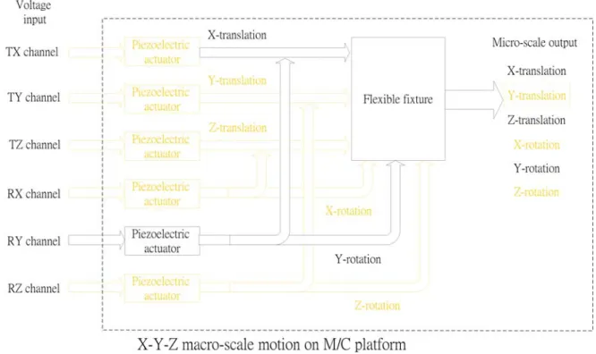
specimen of system experiment. Fig. 17 shows a system block

diagram of two mechanisms resulting in the displacement of

translational X and Z-axis and rotational Y-axis by utilizing a

PZT. By the comparison with Fig.14 containing six freedoms, it

presents the simplification of Fig.17. In terms of the methodology

and providing items of Table 1, parameters of FEM and

experiment are obtained. Due to the elastic material property of

EPFHM, it has difficulties in measuring parameters separately

and accurately. Therefore, according to the methodology of FEM

and experiment, the parameters are derived from Eq. (19) and (20)

that are the system equations of modified parameters with

joint-measurements.

37

Fig. 17 System block diagram of Model 1 and Model 2

5.1. Stiffness Verification of Model 1 & 2

Beginning with analytic K value helps evaluate the maximum displacement in each axis of EPFHM model 1 & 2 and provide the operational resources for experiment reference. The relationship between load and displacement which tends to linearity is derived after the experiment and it also helps the determination of experimental K value.

5.1.1 Model 1

K value is derived from calculating the results of case 1, 2, 3 and 4 by Eq.(18) and it is shown as below.

Case 1:

When

^{= 1}

is loading

The X axial deformation

10

288 .

3 ×

δ = 304.1363 /

Kx

=

,

2 max

0.2617

/

σ =

By utilizing tensile strength (ABS P400 之 σ

^{= 34 . 5}

^/

) as

the calculational datum of a safety coefficient, the maximum deformation is shown as below.

x T

allowable

x SF

δ

σ

δ σ ⋅

= ⋅

max

(48)

This paper specifies that the safety coefficient

in FEM analysis is bigger than 5 and it leads to the strain relation of stress tending to linearity. This is merely assumed to be references for operational use in experiment to prevent the yield deformation of EPFHM. Therefore,

) ( 0867 . 0 10 288 . 2617 3 . 0 5

5 .

34

allowable mm

x

⋅ × =

= ⋅

δ

Case 2:

When

^{= 1}

is loading on

^{= 34}

mm

N M

= 1 × 34 = 34 ⋅

) ( 10 3647 . 34 4 1484 .

0

1

1 Tan rad

Tan r

x z x

−

−

−

= = ×

= δ

θ

And, δ

is z-axial deformation.

rad mm N K_rx

= 7 . 7898 × 10

⋅ /

2 max

0.4310

/

σ =

Therefore, the maximum deformation of z-axial rotation is )

( 38 . 2 1484 . 431 0 . 0 5

5 .

34

allowable

z

⋅ =

= ⋅ δ

Case 3,4:

As same as case 1 and 2 which is illustrated in Table 2.

38

Start with the experiment of displacement and force in order to experiment with

^,

^,

^,

. By utilizing kistler measuring force system, the results of force measurement is shown in Fig. 18 After the calculation of transforming force measurement into moment and rotational displacement, the derivation of

rz ry rx

x K K K

K

, , ,

is shown as below.

mm N K_x

= 49 . 6 /

rad mm N K_rx

= 1 . 1833 × 10

⋅ /

rad mm N K_ry =7.6807×10³ ⋅ /

rad mm N K_rz

= 3 . 8202 × 10

⋅ /

Three rotational axes Rx, Ry, and Rz （ based on the standard of Rz axis）

The ratio of analytic K value is 2.93 : 1 : 3.59 with Rz>Rx>Ry in rigidity order.

The ratio of experimental K value is 15.41 : 1 : 4.97 with Rx>Rz>Ry in rigidity order.

Before the comparison, the discordant of rigidity order between analytic value and experiment one has been confirmed due to several reasons. That is,

1. The rough evaluation by isotropy Young‘s modulus.

2. The different layering precision in X, Y, and Z axes of EPFHM during the process of RP manufacturing.

3. The dissimilar boundary conditions of experiment and analysis.

4. Unexpected deformation occurred beyond the weakness design area.

These above phenomenon results in forming the position of curved surface and uncertain error of EPFHM driven by a PZT.

Meanwhile, it verifies the preceding assumption in proper

direction.

Translation of X-axis

0 10 20 30 40 50 60

0 0.2 0.4 0.6 0.8 1 1.2

Displacement(mm)

Force(N) Rotation about X-axis

0 5 10 15

0 0.1 0.2 0.3 0.4 0.5 0.6

Displacement(mm) Force in Z-

direction (N)

(a)in x-direction (b) in rotational x-axis

Rotation about Y-axis

0 0.5 1 1.5 2 2.5

0 0.5 1 1.5

Displacement(mm) Force in Z-

direction(N)

Rotation about Z-axis

0 5 10 15 20

0 0.5 1 1.5 2 2.5

Displacement(mm) Force in

Y- direction(

N)

(c) in rotational y-axis (d)in rotational z-axis Fig. 18 Results of stiffness experiment of RP Model 1: (a)in x-direction, (b)

in rotational x-axis, (c)in rotational y-axis, (d) in rotational z-axis

5.1.2. Model 2

After the analysis of K value, case 1, 2, 3 and 4 is shown in Table 3 and 4. δ

in loading direction provides the reference to pre-pressure while the experiment of EPFHM by a PZT. If the value which combines the displacement of each axis with the value of pressure in advance is below δ

, it helps the quasi-linear structure of EPFHM. The result of experiment is shown in Fig.19 and K value is obtained as shown as below.

mm N K_x

= 55 . 17568 /

rad mm N K_rx

= 24105 . 02 ⋅ /

rad mm N K_ry

= 5053 . 315 ⋅ /

rad mm N K_rz =195444.2 ⋅ /

40

Table 3 Property analysis on linear structure of EPFHM Model 1

Case Load Motion type Loading direction

Moment (

⋅

) Displacement )

max

(

δ

Displacement in motion type

Stiffness type

) /

(

max N mm

σ δ

^{(mm )}

in loading direction 1 1N x-translation x 3 . 288 × 10

∆

= 3 . 288 × 10

= 304.1363

/ 0.2617 ^0.0867 2 1N x-rotation -z

= 1 × 34 = 34 0.1484

4.3647 10

x rad

θ = ×

= 7.7898 10 ×

⋅ / 0.4310 2.38 3 1N y-rotation -z

74 74 1 × =

y

=

M

0.2011

y

= 0 . 0028

θ

1.272 1.09

4 1N z-rotation y

0.0576

7.7797 10

z rad

θ = ×

= 9.5129 10 ×

⋅ / 0.8914 0.446

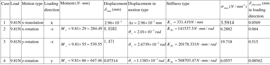
Table 4 Property analysis on linear structure of EPFHM Model 2

Case Load Motion type Loading direction

Moment (

⋅

) Displacement )

max

(

δ

Displacement in motion type

Stiffness type

) /

(

max N mm

σ δ

^{(mm )}

in loading direction 1 9.81N x-translation x 2 . 96 × 10

∆

= 2 . 96 × 10

= 331 . 419

/

3.5914 ^0.0569 2 9.81N x-rotation -z

= 9 . 81 × 29 = 284 . 49 0.0583

x rad

10

01 .

2 ×

θ =

^{= 141537 . 5}

^⋅

^/

6.2882 0.064 3 9.81N y-rotation -z

55 . 539 55 81 .

9 × =

y

=

M

1.471

y rad

10 2

6739 .

2 × ⁻

θ = K_Ry

= 20178 . 331

⋅

/

19.718 0.515

4 9.81N z-rotation y

0.07514

6.0557 0.08562

Three rotational axes Rx, Ry, and Rz （ based on the standard of Rz axis）

The ratio of analytic K value is 6.50 : 1 : 27.07 with Rz>Rx>Ry in rigidity order.

The ratio of K value indicates that the conspicuous displacement in rotational y-axis is occurred by a PZT.

Translation of X-axis

0 10 20 30 40 50 60

0 0.2 0.4 0.6 0.8 1 1.2

Displacement(mm)

Force(N) Rotation about X-axis

0 5 10 15

0 0.1 0.2 0.3 0.4 0.5 0.6

Displacement(mm) Force in Z-

direction (N)

(a) F-x for Kx (b) F-z for Krx

Rotation about Y-axis

0 0.5 1 1.5 2

0 0.2 0.4 0.6 0.8 1 1.2

Displacement(mm) Force in Z-

direction(N )

Rotation about Z-axis

0 10 20 30 40 50

0 0.2 0.4 0.6 0.8 1 1.2

Displacement(mm) Force in Y-

direction(N)

(c) F-z for Kry (d) F-y for Krz

Fig. 19 Results of stiffness experiment of RP Model 2: (a)in x-direction, (b)

in rotational x-axis, (c)in rotational y-axis, (d) in rotational z-axis

42

5.2. FEA and experiment of system property

According to the methodology in Table 2, analytic and experimental items include: (1) the quantity examination regarding to the performance of voltage by PZT displacement, and (2) the qualitative analysis in relation to the allowed movement length of EPFHM, the prior position of PZT, and the influences of variation on spacer ’s friction coefficient.

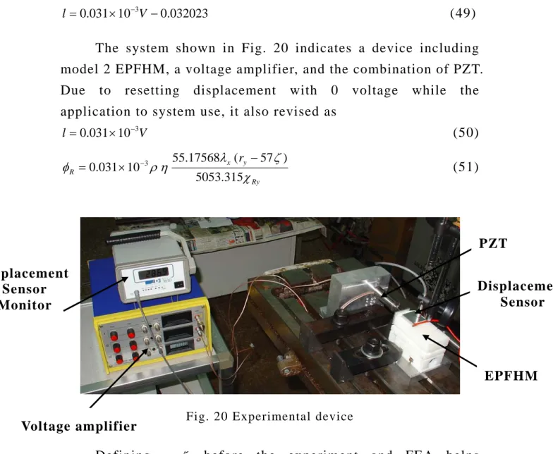
After the experiment of

=

(V ) in a PZT, the quasi-linear is 032023

. 0 10

031 .

0 ×

−

=

l

(49) The system shown in Fig. 20 indicates a device including model 2 EPFHM, a voltage amplifier, and the combination of PZT.

Due to resetting displacement with 0 voltage while the application to system use, it also revised as

V

l

= 0 . 031 × 10

(50)

Ry y x R

r

χ

ζ η λ

ρ

φ 5053 . 315

) 57 ( 17568 . 10 55

031 .

0

−

×

=

(51)

Fig. 20 Experimental device

Defining

, ζ before the experiment and FEA helps determine the proper position and spacer of a PZT. Fig. 21(a) shows the unsatisfactory results of analyzing output condition of Voltage amplifier

PZT

Displacement Sensor

EPFHM Displacement

Sensor

Monitor

working platform and Fig. 21(b) illustrates the quasi-linear output.

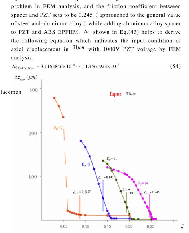
According to the determination of displacement and precision level by the ratio of input and output, Fig. 22 reveals the friction coefficient in a cross axis and the maximum displacement in a vertical axis after the analysis of FEA. With the variation of

in quasi-linear displacement, the maximum deformation is occurred from the aftertreatment figure of FEA. Therefore, the linear area shown in Fig. 22 excluding the horizontal level tends to be identical with tendency of analysis and experiment and that is also the controllable area for experimental use. On the other hands, with less friction coefficient followed by the less

, the displacement of EPFHM tends to be more stable with higher gradient of linear slope, and vice versa. Choosing the maximum

mm

r_y

= 14 as the position of a PZT and polished aluminum alloy as a spacer coordinated with PZT obtains the conditions towards

2456 .

= 0

ζ . Therefore, Eq.(52) is derived from Eq.(51) and Eq.(43) is revised as Eq.(53) which are shown as below.

Ry x

R

χ

ζ η λ

ρ

φ

) 57 14 ( 17568 . 10 55

031 .

0 × ³ −

= ⁻

(52)

r z

Ry

⋅ +

− ⋅

= ×

∆ 3 . 3848 10

( 14 57 ) ( ε ) χ

ζ ρη

(53)

44

(a)discontinuous deformation

(b)linear deformation

Fig. 21 The output condition of working platform: (a)discontinuous

deformation (b)linear deformation

5.3. Estimation equation through input/output system of finite element method

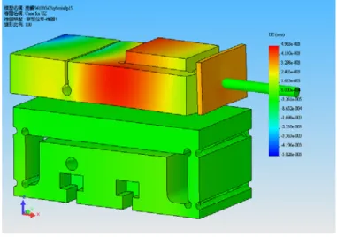
By the reference of Fig. 20, it indicates that the system equation is evaluated by the boundary condition of contract problem in FEM analysis, and the friction coefficient between spacer and PZT sets to be 0.245（ approached to the general value of steel and aluminum alloy） while adding aluminum alloy spacer to PZT and ABS EPFHM. ^∆

shown in Eq.(43) helps to derive the following equation which indicates the input condition of axial displacement in 31 µ

with 1000V PZT voltage by FEM analysis.

3 5

1000 =3.1153846×10⁻ ⋅ +1.4561923×10⁻

∆z_{FEAin V} r

(54) Due to the quasi-linear property of PZT, the system equation is derived shown as below.

V r

z_FEA

= × ⋅ + ⋅

∆ 3 . 1153846 10

( 46 . 7420 ) (55)

Friction coeffiecient

Fig. 22 Diagrm of maximal displacement versus friction coeffiecient in FEA mechaning process

Displacemen

46

5.4. The input and output system equation based on experiment

Fig. 21 shows the experimental diagram of

and

1000

~

0

. Due to the displacement of PZT and deformation of EPFHM within the range of quasi-linear, the experimental system equation is derived shown as below.

V r

z_Experiment = × ⋅ + ⋅

∆ 5.0912 10⁻⁸ ( 23.2892)

(56) Therefore, the voltage of distinct position and height is derived from the following equation.

2892 . 8 23

. 19641734

+

⋅ ∆

=

V z

(57)

Fig. 23 Measured height-voltage Characteristic composed of RP Model 2 flexure hinge mechanism and piezoelectric actuator: (a).

Linear plotting; (b) Linear plotting without data in 1000V; (c) B-spline type plotting without data in 1000V.

5.5. The comparison of system input and output based on FEM and experiment

Eq.(55) is revised as Eq.(56) and also shown in Eq.(58) based on FEM and experiment.

V r

z

=

× 3 . 1153846 × 10

( +

× 46 . 7420 )

∆ β

β (58)

And, β , and

β are modified constants; therefore,

6342

.

= 1

β

, β

= 0 . 4982

V r

z_Experiment =1.6342×3.1153846×10 ⁸ ( +0.4982×46.7420)

∆ ⁻

(59)

5.6. Generating controlled position of curved surface

Under the situation with lots of existing limits, generating a curved surface is verified by Ruled surface and Conical surface according to the design methodology.

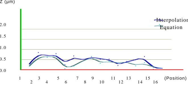
5.6.1 The Ruled forming surface

Generating a curved surface with input voltage of 0V to 1000V in this paper is shown in Fig. 23 And the determination of each voltage point is based on two methods: interpolation and Eq.(57). The assumed measurement of 16 points on a workpiece respectively fits with z-axial coordinates after PZT-driven. The error comparison of these two methods is shown in Fig. 24 And the result reveals that the operational voltage of each point is promptly derived from the calculation. Fig. 25 shows a superimposed diagram of curved surface in relation to the values of experiment and target.

Fig. 24 The error comparison of average equation and ruled forming surface.

Z (µm)

(Position) 1.0

0.5 1.5

0.0

2.0

Interpolation

Equation

1

2 3

4 5

6 7

8 9

10 11

12 13

14 15 16

48

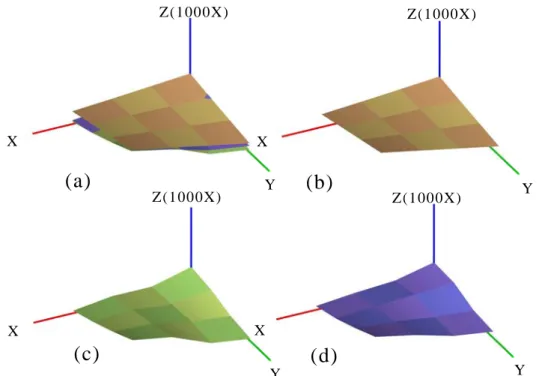
Fig. 25 Ruled forming surface： (a) Three repetition of target, interpolation voltage, and average voltage; (b) target surface; (c)

the forming surface of interpolaton voltage; (d) the forming surface of average voltage

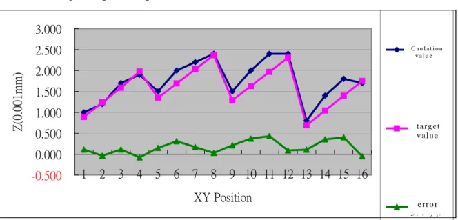
5.6.2. The Conical forming surface

Based on Eq.(57), it helps determine 16 points measurement of driven voltage expressed in a caulation value segment and target values in a target value segment of Fig. 26 The error value segment indicates the error between measurement and target values within 0.4 µ . In Fig. 27 shown as the geometric ratio of Conical forming

surface regarding to experiment and target, Fig. 27(a) indicates a superimposed curved surface generated by the voltage of target value and system equation. Fig. 27(b) is regarded as target surface, while Fig. 27(c) signifies a curved surface generated by the voltage of system equation according to fitting operation. And Fig. 27(d) shows a curved surface generated by the voltage of system equation

Z(1000X) Z(1000X)

Z(1000X) Z(1000X)

X

X

X

X

Y Y

Y Y

(a)

(c)

(b)

(d)

according to spline operation.

-0.500 0.000 0.500 1.000 1.500 2.000 2.500 3.000

1 2 3 4 5 6 7 8 9 10 11 12 13 14 15 16 XY Position

Z(0.001mm)

數列1

數列2

數列3

Fig. 26 The comparison of caulation value, target value, and error.

Fig. 27 Conical forming surface： (a) The repetition of target and average voltage; (b) Target surface; (c) The forming surface A of average voltage;

(d)The forming suface B of average voltage

Vo l t a g e = 0 Vo l t a g e = 0

Vo l t a g e = 0 C o n s t r u c t e d s u r f a c e b y s p l i n e o p e r a t i o n C o n s t r u c t e d s u r f a c e b y f i t t i n g o p e r a t i o n

P r a c t i c a l m e a s u re d p o i n t C o n i c a l ta r g e t s u r f a c e C o n i c a l ta r g e t s u r f a c e

X

X X

X Z（ 1 0 0 0 X ）

Y Y

Y Z（ 1 0 0 0 X ）

Z（ 1 0 0 0 X ）

Z（ 1 0 0 0 X ）

Y Vo l t a g e = 0

C a u l a t i o n v a l u e

t a rg e t v a l u e

e r r o r