利用其他遊戲的經驗來加速新遊戲的訓練

(1)

國立臺灣大學電機資訊學院資訊工程學系碩士論文

Department of Computer Science and Information Engineering College of Electrical Engineering and Computer Science

National Taiwan University Master Thesis

利用其他遊戲的經驗來加速新遊戲的訓練

LEVERAGE EXPERIMENTS FROM OTHER TASKS TO SPEED UP TRAINING

李盈 Ying Li

指導教授：徐宏民博士 Advisor: Winston H. Hsu, Ph.D.

中華民國 107 年 9 月

September, 2018

(2)

(3)

誌謝

首先，非常感謝我的家人們對於我的支持與鼓勵。也非常感謝我的指導教授 Winston 不厭其煩的指點及引導。感謝李宏毅老師協助我入門強化學習的領域，感謝 Winston 和其他實驗室老師們爭取來了強大 GPU 資源，感謝兩屆網管們吳逸群和楊碩碉對於環境設定的鼎力相助，感謝蘇宏庭學長、林之宇等實驗室同學提供我許多寶貴的研究方向及建議，感謝李胡丞、江泓樂、李冠穎學長等同學們協助我理順絲路、排練口試、撰寫論文等等，感謝宿舍室友們以及教會的禱告大軍一路相隨。感謝有這麼多人的鼎力相助，我的研究才終於走到了今天。

唯願一切的榮耀都歸於上帝，感謝有祂一路陪伴與指引，讓我有機會一窺我們習以為常的「歸納學習」是何等困難！

(4)

摘要

雖然深度強化學習（RL）的方法已經在各種視頻遊戲上達到了令人印象深刻的成果，但是 RL 的訓練仍然需要許多時間和計算資源，基於通過隨機探索環境，並從對應的稀疏獎勵中提取信息非常困難。已經有許多作品試圖通過利用以往經驗中的相關知識來加速強化學習過程。有些人認為這是一個轉移學習問題，試圖利用其他遊戲的相關知識。有些人認為這是一個多任務問題，試圖找到一些能夠推廣到新任務的表示方法。在這篇論文中，我們將 agent 與環境互動並收集經驗的過程，視作生成訓練數據的方式，我們需要讓訓練數據擁有更多的差異，以使訓練過程更有效。然後，我們嘗試將在其他遊戲環境中訓練的模型加載到我們想要訓練的新遊戲中，以便生成一些不同的訓練數據。結果表明，使用不同目標的其他遊戲而不是隨機採取行動的策略可以加快學習過程。

關鍵字：強化學習

iv

(5)

Abstract

Although the deep reinforcement learning (RL) approach has achieved impressive results in a variety of video games, training by RL still requires a lot of time and computational resources since it is difficult to extract information from sparse reward by random exploration with the environment. There have been many works attempts to accelerate the RL process by leveraging relevant knowledge from past experience. Some formulated this as a transfer learning problem, exploiting relevant knowledge from other games. Some formulated this as a multitasking problem, tried to find some useful repre- sentations which are capable of generalizing to new tasks. In this work, we treat the process the agent interacts with the environment and collects experience as a way to generate training data, which needs more variance to make the training process more efficient. We then try to load models trained on other game environments to the new game we want to train, in order to generate some different training data. The results show that use policy from other games with different goals instead of randomly taken action could speed up the learning process.

Keywords: Reinforcement Learning

(6)

List of Figures

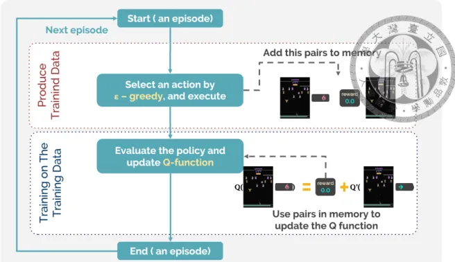
3.1 The Framework for Double DQN: We could consider the process of in- teracting with the environment than collect the experiences, as the process of generating data for training. Refer to Sec. 3 for details. . . 7

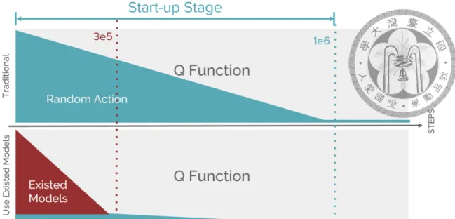
3.2 The Training Data Produced: Here we show the policy that the agent takes when generating training data. The upper graph shows that as the training time increases, the probability of randomly selecting actions will decrease, and the learned policy will be selected. The lower graph shows that if we use the policies of the existing models during the startup phase, we will get more different and goal-oriented training data. (Note that the two numbers 3e5 and 1e6 represent the required steps. More detailed settings will be shown in the experimental setting. Refer to Sec. 4.1 for details.) . . . 8

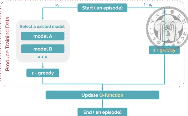
3.3 The Framework to use existing models: Refer to Sec. 3.1 for details. . 9 viii

(9)

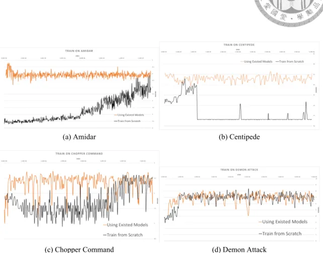
4.1 Comparison between using existing models or not: Black lines are tra- dition method, orange lines are leveraging experience from existing models. The existing models are trained on Air Raid, Alien, Amidar, Cen- tipede, Chopper Command, Bank Heist, Battle Zone, Carnival, Demon Attack, Solaris, Space Invaders, Star Gunner, and Venture. Note that one game will NOT take the model trained from itself as one of the existing models, hence each game has 12 existing models in our experiments.

Leveraging experience from existing model could make the startup phase more efficiently. Moreover, in some game such as (b), experience under random decision cannot support enough information for DDQN to induce, while DDQN could learn from experience from some other models successfully. . . 15 4.2 Comparsion between finetuning from existing models and leveraging

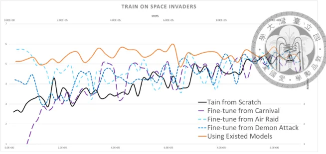
experiments from existing models: the orange line is leveraging from 3 existing models, Carnival, Air Raid, and Demon Attack. The result shows that simply finetune from existing models cannot help us to shorten the startup phase. To finetune from one of the existing models, we first initialize the parameters of the Q Network by the selected model, then follow the same process as training from scratch. Refer to Sec. 4.3 for details. . . 16

(10)

List of Tables

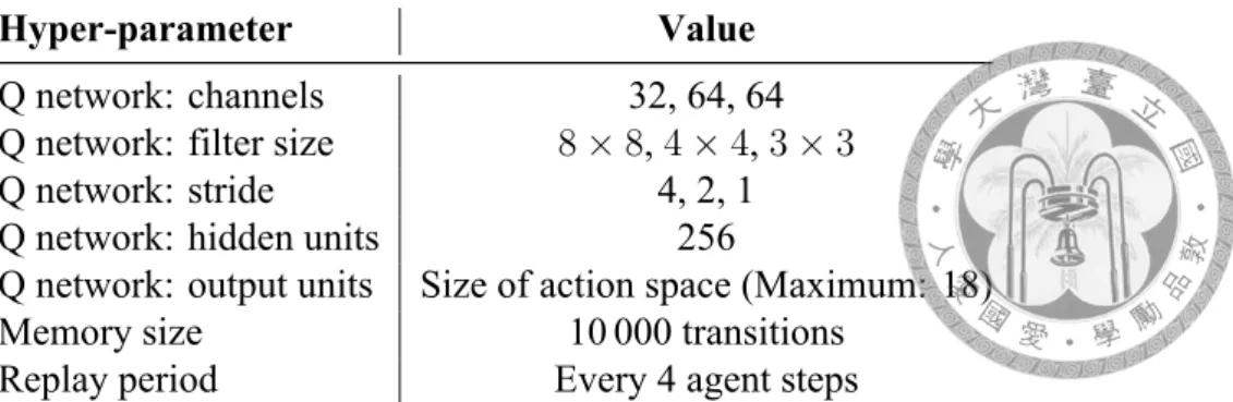
4.1 Hyper-parameters: the values of these hyper-parameters are the same in all the experiments. The network has 3 convolutional layers: with 32, 64 and 64 channels. The layers use 8× 8, 4 × 4, 3 × 3 filters with strides of 4, 2, 1, respectively. Note that we have only 256 units in our hidden layer, as in [7], not 516 units as in the original DQN paper [24] and DDQN paper [34]. Moreover, the maximum number of transitions stored in the memory is much less than in [34] (1M transitions), since the device we use could not afford more. . . 14 4.2 Directly load existing model to another game: we have 3 existed mod-

e, trained from scratch on Demon Attack, Carnival, and Space Invaders respectively. These 3 games are all shooting game with 6 actions available. This table shows the average scores of 300 rounds of each game, loading one of the existing models than play directly without finetuning.

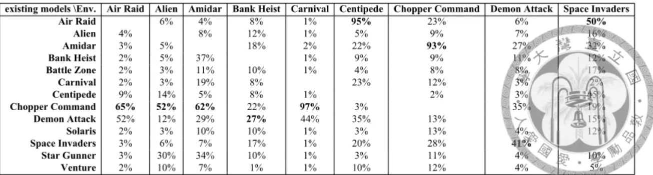
We set the average score of using the model trained on the original game as 100%. The result indicates that sometimes the model trained on one game are suit for the other game. Refer to Sec. 4.3 for details. . . 16 4.3 Most Valuable Player: The proportion of times an existing model (Col-

umn) had been selected to train a game (Row). Refer to Sec. 4.4 for more details. . . 17 4.4 The Screenshot and the size of action space for each game (on the list of

existing models). . . 18

x

(11)

Chapter 1 Introduction

With thriving of deep reinforcement learning (RL) on innumerable areas, such as Atari [24], playing Go [30], controlling continuous systems in robotic systems [21], and video games [35], there has been a dramatic growth in attention and interest. Recent years, researchers have to start to pay attention to some potential issues that can no longer be ignored. [10] pointed out that reproducing results for state-of-the-art deep RL methods are seldom straightforward. [14] addressed some challenges in RL, helping others to set realistic research expectations. Some of these challenges are list as follows:

• Sample inefficient

• The results sometimes will be overfitting to weird patterns in the environment

• The final results may be unstable and hard to reproduce

In our opinion, the main reason for these problems is the way an RL agent explore the environment. People would not explore a new environment completely random. Holding a goal in hand helps a lot, even though this goal is usually different from the current task.

Before finding out how to teach an agent how to explore a new environment efficiently, we tried to let the agent explore the environment with an old goal. It is not necessary for this goal to be similar to the current one, the role of this goal is intended to guide the agent to interact more systematically with the environment more organized, and try not to have such many vague experiments.

(12)

We have some toy experiments to observe the behavior of loading models trained on one Atari game and play with those observations in the other Atari game. Some modes are working! It is needed to train from scratch for each Atari game separately. However, there are some components in common across games. Unlike some works discussed how to define these common parts, such as Hierarchical RL [17], we want to simply use these existed goals from other games to accelerate the training of a new game. In our work, we

load models that were trained in other games directly to generate transitional triples for training. In the initial stage of training, we let our agent hold goals and perspectives from existed models rather than random exploration. This could cause our agent to understand the new environment more efficiently and speed up our training.

In this work, we show that once the agent has some reasonable goals, it will have the opportunity to explore a new environment more efficiently. Though that some of these goals seem to be not similar to the real one, they are much better than random exploration.

2

(13)

Chapter 2 Related Work

2.1 Hierarchical Reinforcement Learning

To improve sample efficiency of unknown tasks, some recent works [17, 9, 27] attempt to define a set of lower-level policy over atomic actions to satisfy the given goal, which could be used for different tasks. These methods tried to provide an abstract state space or a way to define a set of sub-goals. It is very important and very useful to let agents learn by analogy. However, it is too difficult to take a small step. In fact, this field, called hierarchical reinforcement learning, started even before 2000 [31, 26]. Researchers have tried many ways to learn hierarchical policies given various manual specifications, such as a set of sub-goals [31, 26], low-level-skills [13, 3, 20], and state abstractions [11, 15, 16].

In recent works, the state abstraction in [27] is provided by experts, and [17] also uses handcrafted sub-goals for specific tasks. [9] tries to learn a master policy and several fixed-length sub-policies that could not be automatically terminated.In our work, we want a simpler and more versatile way to improve sample efficiency.

2.2 Learning from Demonstration

Learning from expert demonstrations, which is known as behavioral cloning in traditional RL literature, has been tried by many researchers to solve complex tasks. A recent work[2]

tries to let agent learn from human demonstrators from Youtube videos, while the most

(14)

challenge part is not to imitate but to deal with the domain gap between the Arcade Learn- ing Environment [23] and given videos. Such methods attempt to imitate the trajectories have another strong limitation: the agent learning through imitation cannot adapt to the new situations, as described in [1].

2.3 Transfer Learning and Multi-task learning

There is a problem in RL that has been discovered for a long time, a well-trained model and even a problem definition can only be applied to a single task. Since the 1990s, there have been many attempts to apply the idea of transfer learning to RL tasks, and in 2009 there was a survey report on RL transfer learning [32]. As described in [32], the researchers believe that not only generalization can be carried out in tasks, but also generalization between tasks, thus effectively speeding up learning. However, after nearly two decades, which parts should be transferred from which sources, and how to do this, have not been well resolved.

In order to define what should be transferred, some researchers try to define an em- bedding for states, actions or the task, such as [25, 4, 22]. Some motivated by the idea of the student-teacher paradigm introduced by Knowledge Distilling [12], make existing models to be the teachers for a multi-task agent to shorten the time to adapt to the new environment, such as [28, 33, 29, 36, 5].

Whether the researchers want to transfer something from one task to another, or if they want to do multi-task training, the definition of the common part remains a problem.

Furthermore, [8] points out the importance of prior knowledge, claimed that general priors, such as the importance of objects and visual consistency, are critical for efficient game- play. This claim, which was supported by experiments, reveas the fact that this problem is much more difficult than the researchers known.

One of the most similar works with ours is [19]. This work defines a framework for dynamically reusing source policies during training. However, like other transfer learning methods, this work has significant limitations on the source policies: the same action space and the same state space as the new task. Even simple as Atari games are not suitable for

4

(15)

this assumption. In fact, this work only experiments on a series of navigation tasks in the same environment. To make this framework more versatile, we relaxed the restrictions by setting the problem as a goal-oriented exploration rather than reusing source policies.

We want to take advantage of the models we’ve trained as well, while we don’t think it is necessary to extract common components between tasks before doing so.

(16)

Chapter 3 Method

Here, we consider the process of collecting experience as a process for generating training data, as shown in Fig. 3.1. Therefore, the process of evaluating the policy and updating the Q-function could be considered as the process of training on generated training data.

As shown in Fig. 3.2, the training data generated by the traditional method only comes from the Q-Function which are not yet well-trained, and the random policy without a target. In this way, we need to spend a lot of steps in the startup phase to get a few successful experiences. Most training data generated by random policy has less information, which makes it difficult for an agent to introduce some rules. Here, we want to spend most of the steps in the startup phase to use those policies from the existing models, which are trained on other Atari games, instead of random policy. These policies will have different goals because they are designed for different games and have different perspectives since the screen will vary from game to game. To observe the influence of those policies trained on other games, we directly load the model trained on one game, say game A, to the other game B. We found that sometimes the policy from game A will work on game B, and the way the agent solve game B will be different with using the policy trained on game B. We assume that using the policy trained on other game will cause the agent to make a different decision in the same situation and that the decision should be reasonable since the agent has a goal to achieve. Whether or not this goal is similar to the real goal of the current game, keeping a goal during the game may result in more information on the training data generated.

6

(17)

Figure 3.1: The Framework for Double DQN: We could consider the process of inter- acting with the environment than collect the experiences, as the process of generating data for training. Refer to Sec. 3 for details.

Inspired by [19], we use the existing policies to interact with the current environment directly, rather than loading one of the existing models as initial values. Though [19] has strong limitations on the method they proposed, each source policies should have the same action space and state space as the task currently being solved, we could still use the same framework as proposed in [19] since the reason for our use of the old policies are different.

[19] and many other works want to leverage from those learned policies, based on the assumption that some common sense is hidden in learned policies which are useful for the current task. While in this work, we only want some policies that are different from the random policy and the Q-function being updating. We assume that to use centain policies under different goals in the same environment could produce some different experiences.

These different experiences could increase the diversity of our training data, and make our training more effective. The experimental results in Sec. 4 shows that those training data generated by policies trained on other games will make training easier than generated by random policy.

(18)

Figure 3.2: The Training Data Produced: Here we show the policy that the agent takes when generating training data. The upper graph shows that as the training time increases, the probability of randomly selecting actions will decrease, and the learned policy will be selected. The lower graph shows that if we use the policies of the existing models during the startup phase, we will get more different and goal-oriented training data. (Note that the two numbers 3e5 and 1e6 represent the required steps. More detailed settings will be shown in the experimental setting. Refer to Sec. 4.1 for details.)

3.1 System Framework

In our approach, we will have one or more pre-trained models, each of them were trained in a single game. The only limitation on the games they trained in is the game should be one of the 59 Atari games supported by [6]. Therefore, by using the Deep Q-Network algorithm (DQN, [24]), we could place models under a similar architecture. One of the important contributions of DQN is that we could train in different games with one architecture and the same hyper-parameters. All models have 3 convolution layers and 2 fully-connected layers. The only difference between models is the size of the final fully- connected layer, depending on the size of the action space of the game it trained in, refer to Sec. 4.1. We will introduce the method we use to overcome this difference in Sec. 3.3.

This similar network architecture and mapping from different action space make us able to directly load one model trained on game A to play directly in game B. As illustrated in Fig. 3.3, this is almost the same as the framework in[19], we will put all the models available in the pool. Each time before a new episode of the game begins, the agent will

8

(19)

Figure 3.3: The Framework to use existing models: Refer to Sec. 3.1 for details.

have a probability p_t, which will decrease over time, to select a model in the pool. Oth- erwise, the agent will enter the traditional path of Q-Learning (the right path in Fig. 3.3), using the Q-function in training, as shown in Alg. 1. When the agent obtains a policy, from an existing model or the policy which will be updated through time, there is another probability of ϵ to be evaluated every time step. The agent will have a probability of ϵ to select an action randomly or select the best action based on the policy it obtains.

To train the agent by the Q-Learning method, here we use Double Q-Learning (DDQN, [34]), update the policy πq_funcusing the loss

(R_t+1+ γ_t+1q⁻_θ(S_t+1, a^′)− qθ(S_t, A_t))²,

where t is a time step randomly selected from the memory, S_tand A_tare the state and the action in time t respectively. The parameters θ of the online network is used to select actions, and the parameters θ⁻of a target network, which is a periodic copy of the online network, will not be directly optimized.

(20)

3.2 Selecting existing models

Once an episode of a game is over, the environment will return a done signal. The agent then needs to choose a policy for the next episode. Here, the problem of selecting a model from existing models without any prior knowledge of the current game is formulated as the multi-armed bandit problem as [19] did. Different policies loaded from different models could be regarded as bandits with stochastic rewards in muti-armed bandit problem. Since the multi-armed bandit problem has been discussed for a long time, there are many simple and effective algorithms that can achieve the optimal logarithmic regret of this problem, such as the UCB family ([18]). UCB1, which is used in Alg. 2, is one of the algorithms in the UCB family. For each policy π_iin existing_models, the number of selected times T_k(π_i) in the previous k episodes (∀j = 1, ..., n) and the average reward Rk(π_i) will be kept. After all the policies in existing_models have been taken once, UCB1 selects the policy π_j with the equation:

j = arg max_i=1...n^∑_k=1...K(R_k(π_i)) +

√

2ln(K) TK(πi))

3.3 Action Space Mapping

To map one action chosen by the policy from an existing model, which is not included in the action space of the current game, we encode each action using a three-dimensional vector and then performs the action in the action space that is closest to the action selected by the given policy. The 18 actions available in Atari games are Not-Move, Up, UpRight, Right, DownRight, Down, DownLeft, Left, UpLeft, Fire, Up-Fire, UpRight-Fire, Right- Fire, DownRight-Fire, Down-Fire, DownLeft-Fire, Left-Fire, and UpLeft-Fire. Those actions could be divided into three group of components:

• Up, Not-Move, Down

• Right, Not-Move, Left

• Fire, Not-Move

10

(21)

Function learning(env, existing_models):

obs← env.reset();

k ← 0;

total_reward← 0;

for each πi in existing_models do T_k(π_i)← 0;

end

policy_use← policy_selection(Tk, Rk, existing_models);

for t = 1 to max_timestep do act← πpolicy_use(obs);

new_obs, rew, done← env.step(act);

Add obs, act, rew, new_obs, done into memory;

total_reward← total_reward + rew;

if done then k ← k + 1;

total_reward← 0;

obs← env.reset();

T_k(π_{policy_use})← Tk−1(π_{policy_use}) + 1;

R_k(π_{policy_use})← total_reward;

With probability p_t: ;

policy_use← policy_selection(Tk, R_k, existing_models);

With probability 1− p_t: ; policy_use← πq_f unc; end

π_{q_f unc} ← train(memory);

end end

Algorithm 1: Q-learning procedure with existing models to explorate at the startup phase

Function policy_selection(TK, R_K, existing_models):

max_j ← 0 ;

for each πi in existing_models do if TK(π_i) = 0 then

return π_K; end

j ← arg maxi=1...n

∑

k=1...K(R_k(π_i)) +

√

2ln(K) TK(πi)) ; return π_j ;

end

Algorithm 2: select policy from existing models

(22)

We encode the components Up, Right and Fire to 1, encode Down and Left to -1, and encode Not-Move to 0. Using this encoding, the action UpRight-Fire will be encoded as (1, 1, 1), actions with the distance 1 to UpRight-Fire are Up-Fire, UpRight, and Right-Fire.

12

(23)

Chapter 4 Experiments

4.1 Experimental Settings

Here, we compare the results of using existing models with the results obtained by the traditional method, based on Baselines provided by OpenAI ([7]), in the Gym environment ([6]). All experiments used the same hyper-parameters listed in Table. 4.1, training from scratch without additional knowledge. When using the traditional method, the agent has a probability of 0.99 to react to the environment with random action (ϵ = 0.99), and this probability will decrease to 0.02 linearly within the first 1 000 000 time steps (ϵ = 0.02).

While in the method to use existing models, the probability to chose from existing models, p, is set to 1.0 at first and decrease to 0.02 linearly within the first 300 000 time steps. ϵ is

set to 0.1 at first and decrease to 0.02 within the first 300 000 time steps.

4.2 Successfully Speed Up Training

As shown in Fig. 4.1, leveraging from existing models successfully shorten the startup phase. Here we trained our model using one Tesla K80 GPU. To collect 100 000 transitions of experience, it spent about 3 hours GPU time. Without the help from other existing models, we need at least 45 hours, 19 hours, and 3 hours to get a model for Amidar, Chop- per Command, and Demon Attack respectively, while we need less than 3 hours for each game now. Moreover, we even have the opportunity to leverage from some of the experi-

(24)

Hyper-parameter Value

Q network: channels 32, 64, 64

Q network: filter size 8× 8, 4 × 4, 3 × 3

Q network: stride 4, 2, 1

Q network: hidden units 256

Q network: output units Size of action space (Maximum: 18)

Memory size 10 000 transitions

Replay period Every 4 agent steps

Table 4.1: Hyper-parameters: the values of these hyper-parameters are the same in all the experiments. The network has 3 convolutional layers: with 32, 64 and 64 channels.

The layers use 8× 8, 4 × 4, 3 × 3 filters with strides of 4, 2, 1, respectively. Note that we have only 256 units in our hidden layer, as in [7], not 516 units as in the original DQN paper [24] and DDQN paper [34]. Moreover, the maximum number of transitions stored in the memory is much less than in [34] (1M transitions), since the device we use could not afford more.

ence generated by existing models to deal with games where DDQN is underperforming, such as Centipede. We guess that experience under random decision in Centipede does- n’t support enough information for DDQN to induce, therefore the black line (train from scratch) of Fig. 4.1b drops immediately after the probability ϵ decrease to 0.02 after the first 100 000 time steps. Each model has its own rules and unique perspective since it was trained in a completely different environment. These models may able to provide some training data from other distributions, and some of them give Fig. 4.1b the opportunity to derive its own rule.

4.3 Simply Finetune From existing models

Here we will show the reason why we don’t simply finetune from an existing model.

As shown in Table. 4.2, some models could perform well on the other game without finetuning. For instance, to play the game Demon Attack, using the model trained on Space Invaders could beat more than 80% of the average score using the model train on Demon Attack itself. However, to finetune from Demon Attack to Space Invaders could not speed up training, as shown in Fig. 4.2. Moreover, we could not figure out which model could works on another game without experiments. We guess that it is because that the algorithm tries to update the Q function before there is enough training data to derive

14

(25)

(a) Amidar (b) Centipede

(c) Chopper Command (d) Demon Attack

Figure 4.1: Comparison between using existing models or not: Black lines are tradition method, orange lines are leveraging experience from existing models. The existing models are trained on Air Raid, Alien, Amidar, Centipede, Chopper Command, Bank Heist, Battle Zone, Carnival, Demon Attack, Solaris, Space Invaders, Star Gunner, and Venture. Note that one game will NOT take the model trained from itself as one of the existing models, hence each game has 12 existing models in our experiments. Leveraging experience from existing model could make the startup phase more efficiently. Moreover, in some game such as (b), experience under random decision cannot support enough information for DDQN to induce, while DDQN could learn from experience from some other models successfully.

(26)

Figure 4.2: Comparsion between finetuning from existing models and leveraging ex- periments from existing models: the orange line is leveraging from 3 existing models, Carnival, Air Raid, and Demon Attack. The result shows that simply finetune from existing models cannot help us to shorten the startup phase. To finetune from one of the existing models, we first initialize the parameters of the Q Network by the selected model, then follow the same process as training from scratch. Refer to Sec. 4.3 for details.

existing model \Playing Env. Demon Attack Carnival Space Invaders Demon Attack 7.92 (100%) 1.98 (15%) 2.27 (41%)

Carnival 3.56 (45%) 13.04 (100%) 4.13 (75%) Space Invaders 6.6 (83%) 2.01 (15%) 5.54 (100%) Table 4.2: Directly load existing model to another game: we have 3 existed mode, trained from scratch on Demon Attack, Carnival, and Space Invaders respectively. These 3 games are all shooting game with 6 actions available. This table shows the average scores of 300 rounds of each game, loading one of the existing models than play directly without finetuning. We set the average score of using the model trained on the original game as 100%. The result indicates that sometimes the model trained on one game are suit for the other game. Refer to Sec. 4.3 for details.

centain rule. While in our work, we do not edit any of the parameters in the existing model. The agent will update its own Q function from scratch, and the role of existing models are demonstrating some interaction with the environment. The more scores one existing model could earn, the more likely it is to be used. The orange line in Fig. 4.2 indicates that the agent has leverage experience from existing models successfully.

16

(27)

existing models \Env. Air Raid Alien Amidar Bank Heist Carnival Centipede Chopper Command Demon Attack Space Invaders

Air Raid 6% 4% 8% 1% 95% 23% 6% 50%

Alien 4% 8% 12% 1% 5% 9% 7% 16%

Amidar 3% 5% 18% 2% 22% 93% 27% 32%

Bank Heist 2% 5% 37% 1% 9% 9% 11% 12%

Battle Zone 2% 3% 11% 10% 1% 4% 8% 8% 17%

Carnival 2% 3% 19% 8% 23% 12% 3% 2%

Centipede 9% 14% 5% 8% 1% 2% 3% 45%

Chopper Command 65% 52% 62% 22% 97% 3% 35% 19%

Demon Attack 52% 12% 29% 27% 44% 35% 13% 15%

Solaris 2% 3% 10% 10% 1% 3% 13% 4% 12%

Space Invaders 3% 6% 7% 17% 1% 20% 28% 41%

Star Gunner 3% 30% 34% 10% 1% 3% 11% 4% 10%

Venture 2% 10% 7% 1% 1% 10% 12% 4% 5%

Table 4.3: Most Valuable Player: The proportion of times an existing model (Column) had been selected to train a game (Row). Refer to Sec. 4.4 for more details.

4.4 Most Valuable Player

We conducted a record of the frequency of one existing model has been select by another game, as shown in 4.3. The 13 existing models have 3 different action space; in addition, they could be roughly divided into two categories, shooting games and maze games (as shown in Table. 4.4, Alien, Amidar, Bank Heist and Venture are maze games, the rest are all shooting games. Note that most of the shooting games we have are vertical shooting, instead of Chopper Command and Star Gunner, which are horizontal shooting). Here, we refer to the most frequently selected model as the most valuable player (MVP) in that game.

We could find that the MVP of a game, not always the one we think looks like that game. The MVP in Air Raid and Carnival is Chopper Command, all of them are shooting games, while Chopper Command is horizontal shooting and the other two games are not.

MVPs in Alien, Amidar, Bank Heist are not maze games.

Likewise, we found that MVPs of Air Raid, Amidar, Carnival, Centipede and Chopper Command have different action space than the game itself. This implies that mapping different action spaces gives the agent more useful options.

(28)

Environments Screenshot Number of Ac-

tions Environments Screenshot Number of Ac- tions

Air Raid 6 Chopper Com-

mand 18

Alien 18 Demon Attack 6

Amidar 10 Solaris 18

Bank Heist 18 Space Invaders 6

Battle Zone 18 Star Gunner 18

Carnival 6 Venture 18

Centipede 18

Table 4.4: The Screenshot and the size of action space for each game (on the list of existing models).

18

(29)

Chapter 5 Conclusion

In this work, we tried to leverage some experiments from other tasks. We used models trained on other games as the policy to explore the current new environment. Experimental results show that even though these models have different goals and different perspectives, they could explore the environment more efficiently than random attempts. There is only one limitation to this approach: we need to provide a common network structure for each task. With this limitation, we could extend this approach to other tasks without additional computational costs or editing our framework. We hope that there will be a way to design a learning path for the RL agent. Before that, we believe that there are still some more efficient but simple ways to explore a new environment.

(30)

Bibliography

[1] K. Arulkumaran, M. P. Deisenroth, M. Brundage, and A. A. Bharath. A brief survey of deep reinforcement learning. arXiv preprint arXiv:1708.05866, 2017.

[2] Y. Aytar, T. Pfaff, D. Budden, T. L. Paine, Z. Wang, and N. de Freitas. Playing hard exploration games by watching youtube. CoRR, abs/1805.11592, 2018.

[3] P.-L. Bacon and D. Precup. Learning with options: Just deliberate and relax. In NIPS Bounded Optimality and Rational Metareasoning Workshop, 2015.

[4] M. Baroni, A. Joulin, A. Jabri, G. Kruszewski, A. Lazaridou, K. Simonic, and T. Mikolov. Commai: Evaluating the first steps towards a useful general ai. arXiv preprint arXiv:1701.08954, 2017.

[5] G. Berseth, C. Xie, and P. Cernek. Multi-skilled motion control. 2018.

[6] G. Brockman, V. Cheung, L. Pettersson, J. Schneider, J. Schulman, J. Tang, and W. Zaremba. Openai gym, 2016.

[7] P. Dhariwal, C. Hesse, O. Klimov, A. Nichol, M. Plappert, A. Radford, J. Schulman, S. Sidor, Y. Wu, and P. Zhokhov. Openai baselines. https://github.com/openai/

baselines, 2017.

[8] R. Dubey, P. Agrawal, D. Pathak, T. L. Griffiths, and A. A. Efros. Investigating human priors for playing video games. CoRR, abs/1802.10217, 2018.

[9] K. Frans, J. Ho, X. Chen, P. Abbeel, and J. Schulman. Meta learning shared hierar- chies. CoRR, abs/1710.09767, 2017.

20

(31)

[10] P. Henderson, R. Islam, P. Bachman, J. Pineau, D. Precup, and D. Meger. Deep reinforcement learning that matters. CoRR, abs/1709.06560, 2017.

[11] B. Hengst. Discovering hierarchy in reinforcement learning with hexq. In ICML, volume 2, pages 243–250, 2002.

[12] G. Hinton, O. Vinyals, and J. Dean. Distilling the knowledge in a neural network.

arXiv preprint arXiv:1503.02531, 2015.

[13] M. Huber and R. A. Grupen. A feedback control structure for on-line learning tasks.

Robotics and autonomous systems, 22(3-4):303–315, 1997.

[14] A. Irpan. Deep reinforcement learning doesn’t work yet. https://www.alexirpan.

com/2018/02/14/rl-hard.html, 2018.

[15] J. Z. Kolter, P. Abbeel, and A. Y. Ng. Hierarchical apprenticeship learning with application to quadruped locomotion. In Advances in Neural Information Processing Systems, pages 769–776, 2008.

[16] G. Konidaris and A. G. Barto. Building portable options: Skill transfer in reinforce- ment learning. In IJCAI, volume 7, pages 895–900, 2007.

[17] T. D. Kulkarni, K. Narasimhan, A. Saeedi, and J. B. Tenenbaum. Hierarchical deep reinforcement learning: Integrating temporal abstraction and intrinsic motivation.

CoRR, abs/1604.06057, 2016.

[18] T. Lai and H. Robbins. Asymptotically efficient adaptive allocation rules. Adv. Appl.

Math., 6(1):4–22, Mar. 1985.

[19] S. Li and C. Zhang. An optimal online method of selecting source policies for rein- forcement learning. CoRR, abs/1709.08201, 2017.

[20] R. Liaw, S. Krishnan, A. Garg, D. Crankshaw, J. E. Gonzalez, and K. Goldberg.

Composing meta-policies for autonomous driving using hierarchical deep reinforce- ment learning. arXiv preprint arXiv:1711.01503, 2017.

(32)

[21] T. P. Lillicrap, J. J. Hunt, A. Pritzel, N. Heess, T. Erez, Y. Tassa, D. Silver, and D. Wierstra. Continuous control with deep reinforcement learning. CoRR, ab- s/1509.02971, 2015.

[22] D. Lopez-Paz et al. Gradient episodic memory for continual learning. In Advances in Neural Information Processing Systems, pages 6467–6476, 2017.

[23] M. C. Machado, M. G. Bellemare, E. Talvitie, J. Veness, M. J. Hausknecht, and M. Bowling. Revisiting the arcade learning environment: Evaluation protocols and open problems for general agents. CoRR, abs/1709.06009, 2017.

[24] V. Mnih, K. Kavukcuoglu, D. Silver, A. A. Rusu, J. Veness, M. G. Bellemare, A. Graves, M. Riedmiller, A. K. Fidjeland, G. Ostrovski, et al. Human-level control through deep reinforcement learning. Nature, 518(7540):529, 2015.

[25] M. Nickel and D. Kiela. Poincaré embeddings for learning hierarchical represen- tations. In Advances in neural information processing systems, pages 6338–6347, 2017.

[26] R. E. Parr and S. Russell. Hierarchical control and learning for Markov decision processes. University of California, Berkeley Berkeley, CA, 1998.

[27] M. Roderick, C. Grimm, and S. Tellex. Deep abstract q-networks. In AAMAS, 2018.

[28] A. A. Rusu, S. G. Colmenarejo, Ç. Gülçehre, G. Desjardins, J. Kirkpatrick, R. Pas- canu, V. Mnih, K. Kavukcuoglu, and R. Hadsell. Policy distillation. CoRR, ab- s/1511.06295, 2015.

[29] T. Shu, C. Xiong, and R. Socher. Hierarchical and interpretable skill acquisition in multi-task reinforcement learning, 2017.

[30] D. Silver, A. Huang, C. J. Maddison, A. Guez, L. Sifre, G. van den Driess- che, J. Schrittwieser, I. Antonoglou, V. Panneershelvam, M. Lanctot, S. Diele- man, D. Grewe, J. Nham, N. Kalchbrenner, I. Sutskever, T. Lillicrap, M. Leach,

22

(33)

K. Kavukcuoglu, T. Graepel, and D. Hassabis. Mastering the game of Go with deep neural networks and tree search. Nature, 529(7587):484–489, Jan. 2016.

[31] R. S. Sutton, D. Precup, and S. Singh. Between mdps and semi-mdps: A framework for temporal abstraction in reinforcement learning. Artificial intelligence, 112(1- 2):181–211, 1999.

[32] M. E. Taylor and P. Stone. Transfer learning for reinforcement learning domains: A survey. Journal of Machine Learning Research, 10(Jul):1633–1685, 2009.

[33] C. Tessler, S. Givony, T. Zahavy, D. J. Mankowitz, and S. Mannor. A deep hierarchical approach to lifelong learning in minecraft, 2016.

[34] H. van Hasselt, A. Guez, and D. Silver. Deep reinforcement learning with double q-learning. CoRR, abs/1509.06461, 2015.

[35] O. Vinyals, T. Ewalds, S. Bartunov, P. Georgiev, A. S. Vezhnevets, M. Yeo, A. Makhzani, H. Küttler, J. Agapiou, J. Schrittwieser, J. Quan, S. Gaffney, S. Petersen, K. Simonyan, T. Schaul, H. van Hasselt, D. Silver, T. P. Lillicrap, K. Calderone, P. Keet, A. Brunasso, D. Lawrence, A. Ekermo, J. Repp, and R. Tsing.

Starcraft II: A new challenge for reinforcement learning. CoRR, abs/1708.04782, 2017.

[36] H. Yin and S. J. Pan. Knowledge transfer for deep reinforcement learning with hierarchical experience replay. In AAAI, pages 1640–1646, 2017.