選擇權隱含波動與股價分配之研究

行政院國家科學委員會專題研究計畫 成果報告

選擇權隱含波動與股價分配之研究

計畫類別： 個別型計畫

計畫編號： NSC93-2416-H-011-009-

執行期間： 93 年 08 月 01 日至 94 年 07 月 31 日 執行單位： 國立臺灣科技大學企業管理系

計畫主持人： 林丙輝

報告類型： 精簡報告

處理方式： 本計畫涉及專利或其他智慧財產權，1 年後可公開查詢

中 華 民 國 94 年 11 月 17 日

行政院國家科學委員會補助專題研究計畫成果報告

選擇權隱含波動與股價分配之研究

Implied Volatility and Stock Price Distribution in Options

計畫類別：

5

執行期間： 93 年 8 月 1 日至 94 年 7 月 31 日

計畫主持人：林丙輝

本成果報告包括以下應繳交之附件：

□赴國外出差或研習心得報告一份

□赴大陸地區出差或研習心得報告一份

□出席國際學術會議心得報告及發表之論文各一份

□國際合作研究計畫國外研究報告書一份

執行單位：國立台灣科技大學企業管理系

中 華 民 國 94 年 11 月 16 日

行政院國家科學委員會專題研究計畫成果報告 選擇權隱含波動與股價分配之研究

Implied Volatility and Stock Price Distribution in Options 計畫編號：NSC93-2416-H-001-009

執行期限：93 年 8 月 1 日至 94 年 7 月 31 日

計畫主持人 ：林丙輝 國立台灣科技大學企業管理系 中文摘要

波動性在金融市場中是風險管理不可或缺的資 訊，也是選擇權評價中最關鍵的變數。而藉著選 擇權市場，不同到期期限與履約價格選擇權契約 的交易，波動性資訊可以適當反映出來。完整的 選擇權市場價格中亦隱含了其標的資產價格風險 中立的分配，特別是偏態係數與峰態係數，在資 產評價、風險管理決策中均扮演著很重要的角色。

Black and Scholes (1973)的模型假設簡單，其評價 與實際市場資料並無法吻合，例如波動性並不是 固定常數，使得標的股價分配並不符合對數常態 分配。因而市場上選擇權的價格呈現履約價格低 的選擇權，其隱含波動較高，履約價格高的選擇

權，其隱含波動較低。此種現象在1987 年以後的

股票選擇權尤為普遍，稱為波動性偏態。此現象 係對映於股價的分配較對數常態分配有較為肥厚 的左尾，亦即偏態係數為負數，與較高的峰態係 數。

股票選擇權市場呈波動性偏態的現象，是否有系 統或規則，對市場很重要的意義。Bakshi, Kapadia, and Madan (2003)提出計算隱含風險中立偏態及 峰態係數的公式，並導出風險中立偏態與峰態係 數與實際股價報酬分配偏態與峰態係數的關係，

主要反映市場風險趨避的因素。其亦證明了風險 中立偏態係數可直接衡量選擇權隱含波動偏態程 度，並探討了個股選擇權與指數選擇權隱含偏態 之關係，可說明指數選擇權為何有較個股選擇權 左偏的風險中立分配。再則，波動性偏態現象是 否與標的股票公司的基本特質有關也是一個重要 的議題。由於槓桿效果常與波動偏態現象連結，

認 為 是 解 釋 此 現 象 的 原 因 之 一 。Dennis and Mayhew (2002)即檢驗橫斷面個股選擇權偏態狀 況是否與個股槓桿比率是否有關。除了槓桿因素 外，股票交易量、公司市值、系統風險等因素是 否與股價偏態分配有關，也是很直接的議題。另 外Bakus, Foresi, Li, and Wu (1997)提出了考慮隱 含偏態與峰態之選擇權定價公式，並可決定選擇 權避險策略。

綜合以上文獻，本研究欲驗證下列幾個假說：

假說一：選擇權隱含股價風險中立分配呈越左

偏，則其隱含波動曲線斜率越陡。而風險中立分 配呈越厚尾，則隱含波動曲線斜率越平。

假說二：期限較短的選擇權波動曲線斜率較期限 較長選擇權波動曲線斜率較陡。

假說三：指數報酬風險中立分配之偏態平均而言 較個股報酬風險中立分配之偏態越為左偏。

假說四：個股選擇權的隱含波動曲線較指數選擇 權的隱含波動曲線有較小的負斜率。

假說五：選擇權的隱含風險中立偏態與峰態係數 與標的股票實際偏態與峰態係數的關係決定於風 險趨避係數。

假說六：個股選擇權的隱含風險中立分配與波動 曲線斜率與其標的股票的槓桿比率與其他個股相 關變數有相關。

本研究針對在英國倫敦證券交易所上市的公司股

票選擇權以及金融時報股價指數 FTSE 100 指數

選 擇 權 進 行 實 證 研 究 。 資 料 來 源 主 要 為 DataStream 資料庫，資料期間為 1991 年 2 月 19

日至2003 年 11 月 23 日。由於英國倫敦選擇權市

場為美國以外最重要的市場之一，加上研究文獻 實證資料不多，因此應為有趣的研究標的。其研 究成果在學術上與對國內選擇權市場之發展應具 有相當之貢獻。

關鍵詞：隱含波動偏態、風險中立偏態、風險中 立峰態、槓桿效果

ABSTRACT

This article provides some empirical evidence on the implied volatility skew in LIFFE equity options. We investigate the structure and characteristic of the risk-neutral skewness relating to implied volatility skew, using prices of individual equity and FTSE 100 index options. Based on the model of Bakshi, Kapadia, and Madan (BKM, 2003), we test several interesting hypotheses and obtain sometimes contrasting empirical results. First, the slope of implied volatility curve is significantly negative for both individual stocks and index options, and the negativity of the slope becomes less for longer-term options. The implied volatility skew can be described by risk-neutral skewness and kurtosis with the former the first-order effect and the later second-order. Moreover, the implied volatility skew for individual stock options is less severe than that

of the index options, and the idiosyncratic component dominates the market component in determining the individual stock risk-neutral skewness. Finally, as we relate the risk-neutral skewness and kurtosis to those for the real return distribution, the risk-aversion parameter comes to play its significant role. The empirical estimation for the risk-aversion parameter is significantly positive and quite consistent in quantity confirming the stable relationship between the real and the risk-neutral moments implied in option prices. Compared to the results of BKM which use S&P 100 index options and stock options traded on the CBOE, our results indicate that for FTSE 100 index and stock options traded on LIFFE, the slope of implied volatility skew is flatter than that of options traded on CBOE.

As a consequence, the coefficients of skewness and kurtosis for explaining the implied volatility slope, as well as the risk aversion parameter for linking the risk-neutral moments to the physical ones, are considerably less for the U.K. market than the U.S.

market.

Keywords: implied skewness, risk-neutral skewness, risk-neutral kurtosis, leverage effect

1. Introduction

The assumption of the Black and Scholes (1973) option pricing formula is that the underlying process follows a Wiener process with constant volatility. As a result, the underlying conditional distribution is log-normal. However, it is hardly able to fit the actual market option prices. For example, volatility may not be constant, so that the underlying distribution is not consistent with the log-normal distribution. It is quite common to observe that implied volatility in the Black-Scholes formula tends to be high for options with lower exercise prices and low for options with higher exercise prices, the so-called implied volatility skew, a phenomenon particularly prevalent in equity option markets after the crash of 1987. As described in Hull (2003), this phenomenon reflects the fact that the stock price distribution exhibits a fat left tail relative to the log-normal distribution, i.e., the skewness is negative and the kurtosis is high.

There are several types of models to adapt the implied volatility skew or smile effect, that mainly focus on the fact that the volatility is non-constant.

The first type of models incorporates the stochastic volatility component into the underlying process.

For example, the stochastic volatility option pricing models of Hull and White (1987) and Heston (1993), and the GARCH option pricing model of Duan (1995) are different types of stochastic volatility models. The second type of models, such as the Jump-Diffusion model of Merton (1976), assumes

the underlying process is a combination of a continuous diffusion process and a jump process.

Since the jump can lead to a change of the volatility of the underlying price, and an asymmetric jump can cause the underlying distribution to skew and exhibit fat tails, the model can explain the volatility skew or smile to some extent. Alternatively, one can use the model admitting that the volatility is non-constant, by assuming the volatility is a time-varying deterministic function. The model uses the option prices observed from the market to recover the deterministic volatility function, or the underlying risk-neutral distributions. It then can use the arbitrage argument that is underlying the Black-Scholes model, to evaluate other derivatives, and to implement risk management. For example, Derman, Kani, and Zou (1996), Rubinstein (1994), Jackwerth (1999, 2000), and Dupire (1994), all incorporate market prices of options with different exercise prices and maturities, and recover the underlying stock price distribution. One of the main economic functions of a complete option market is to recover the risk-neutral distribution, including the volatility, skewness, and kurtosis of the underlying stock prices, which is important for asset pricing, from prices of options with different maturities and exercise prices. One can develop procedures for backing out implied risk-neutral density functions from observed option prices, such as Breeden and Litzenberger (1978), Rubinstein (1994), and Jackwerth (1999).

Volatility as well as skewness or other higher moments of asset price distribution plays a critical role in asset pricing and risk management. Apart from the second moment, for example, Rubinstein (1973), Kraus and Litzenberger (1976), Harvey and Siddique (1999, 2000), and Lin and Wang (2003) all document that the higher moments play an important role in asset pricing. For example, stocks with negative coskewness require higher equilibrium risk premium. So do those with high cokurtosis. On the other hand, Ait-Sahalia and Lo (1998), Bakshi, Cao, and Chen (1997), Bates (2000), Duffie, Pan, and Singleton (2000), Madan, Carr, and Chang (1998), Pan (1999), and Rubinstein (1994) have incorporated the asymmetries in the underlying risk-neutral pricing distribution into the option pricing model.

It is thus critical to understand the behavior of implied volatility skew and its determinants. Among the researches in this area, Bakshi, Kapadia, and Madan (2003) (hereafter BKM) used the results of Bakshi and Madan (2000) to derive several propositions clarifying the relation between implied volatility skew and risk-neutral skewness and

kurtosis. They also specified the relationship of skewness between individual stock options and index options. Dennis and Mayhew (2002) relate the implied risk-neutral skewness to the underlying stock characteristics such as the leverage effect, the systematic risk, size, trading volume, and so on.

Moreover, Backus, Foresi, Li, and Wu (1997) (hereafter BFLW) derived an option pricing formula which incorporates skewness and kurtosis in the model. They also prove that the implied volatility skew dies out as the maturity becomes infinite.

In this study, we investigate several interesting issues concerning the implied volatility skew and risk-neutral moments. First of all, based on theories developed in BFLW and BKM, for options with certain maturity, the more negative the risk-neutral skewness, the steeper is the slope of implied volatility skew. And in the presence of risk-neutral skewness, the greater the risk-neutral kurtosis, the flatter is the implied volatility slope. However in the absence of risk-neutral skewness, the greater the risk-neutral kurtosis, the steeper is the implied volatility slope. That is to say that skewness plays the first-order role in determining the implied volatility skew, while kurtosis has the second-order effect on it. BKM use CBOE options data to perform empirical examinations and confirm the theory.

Secondly, according to the BFLW model, the implied volatility slopes for shorter-term options are steeper than that for longer-term options. This is quite a common phenomenon observed by many researchers including the BKM and BFLW, and also consistent with Duque and Lopes (2003) using LIFFE options. Third, risk-neutral distributions recovered from individual stock options are, on average, less negatively skewed than that from the market index options. This is also confirmed by the empirical results of BKM. Similarly, the natural consequence is that the implied volatility curves should be less negatively sloped for individual stock options than for stock index options. After conducting a regression analysis, BKM conclude that the idiosyncratic skew is more important than the market skew in explaining the individual stock skew. And it may be directionally offsetting the negative market skew, resulting in the individual stock skew less negative than the market skew.

Finally, also based on BKM, the relationships between the risk-neutral skewness (kurtosis) and the physical return skewness (kurtosis) are determined by the coefficient of relative risk-aversion.

Our samples are individual stock options and the FTSE 100 index option (ESX) traded on the

London International Financial Futures and Options Exchange (LIFFE). Due to limited empirical evidence in the literature, especially outside the U.S.

market, the results of this study provide interesting empirical evidence to the literature. Besides, thanks to extensive empirical results of BKM, we are able to make rigorous comparisons between the UK LIFFE options market and the US CBOE options market in relation to the implied volatility skew, and obtain some interesting empirical implications.

Compared to the results of BKM which use S&P 100 index and stock options traded on the CBOE, our results indicate that for FTSE 100 index and stock options traded on LIFFE, the slope of implied volatility skew is flatter (less negative) than that of options traded on CBOE. As a consequence, the coefficients of skewness and kurtosis for explaining the implied volatility slope, as well as the risk aversion parameter for linking the risk-neutral moments to the physical ones, are considerably less for the U.K. market than the U.S. market.

2. Recovering Implied Risk-Neutral Moments in Options

To see how the implied risk-neutral distribution can be recovered from option prices which exhibit the implied volatility skew, we first focus on the Black and Scholes (1973) model. Under the Black-Scholes (1973) assumptions, the underlying stock price, S(t) follows the process,

( ) ( , , ) ( ) ( )

dS t adt t K dW t

S t = +σ τ (1) where a is the expected rate of return on holding the stock, W(t) is a standard Wiener process;

(σ τ( , , )t K ) is the underlying stock price volatility, which may be a deterministic function of exercise price and maturity. According to risk-neutral pricing paradigm, the price of a call option on a non-dividend paying stock is equal to its discounted expected payoff under the risk-neutral measure:

( , , ) *[max( ( ) , 0)]

max( ( ) , 0) ( ( )) ( )

r t r

C t K e E S t K

e S t K q S t dS t

τ τ

τ τ

τ τ τ

−

− ∞

−∞

= + −

= ∫ + − + +

(2) where q S t( ( +τ)) is the risk-neutral probability density for the distribution of the stock price at time

t+τ , K is the exercise price, τ is the time to maturity of the option, r is the risk-free interest rate, and E^* is the expectation operator with respect to the risk-neutral probability measure.

According to Breeden and Lizenberger (1978), in a complete option market where a full series of options with a continuum of different exercise prices are traded, we can take the partial derivative of the option with respect to its exercise price (K) and obtain:

∫^∞

− + +

−

∂ =

∂

K

r q S t dS t

K e

C ^τ ( ( τ)) ( τ) (3)

We then can further take the second derivative of the option price with respect to the exercise price to obtain the risk-neutral probability density of the stock price distribution when it is at the level of K:

2 2

)

( K

e C K

q ^r

∂

= ^τ ∂ (4)

Thus, when there is a complete set of option series traded in the market, the risk-neutral probability distribution of underlying stock price, as well as the volatility function as in equation (1) are embedded in the option prices. This provides a basis to analyze the option implied risk-neutral volatility and the higher order of moments. However as we are only interested in some moments of the risk-neutral density, rather than the entire density, we can apply the BKM method to measure the risk-neutral moments of interest.

Utilizing the payoff replicating principle, BKM use continuous out-of-the-money (OTM) put and call option prices to compute theτ-period risk-neutral skewness of the underlying asset. That is:

* * 3

* * 2 3/ 2

3 2 3/ 2

{( ( , ) [ ( , )]) } ( , )

{ ( ( , ) [ ( , )]) }

( , ) 3 ( , ) ( , ) 2 ( , ) [ ( , ) ( , ) ]

t t

t t

r r

r

E R t E R t SKW t

E R t E R t

e W t t e V t t

e V t t

τ τ

τ

τ τ

τ τ τ

τ µ τ τ µ τ

τ µ τ

≡ −

−

− +

= −

(5)

And the risk-neutral kurtosis is:

* * 4

* * 2 2

2 4

2 2

{( ( , ) [ ( , )]) } ( , )

{ ( ( , ) [ ( , )]) }

( , ) 4 ( , ) ( , ) 6 ( , ) ( , ) 3 ( , ) [ ( , ) ( , ) ]

t t

t t

r r r

r

E R t E R t KUT t

E R t E R t

e X t t e W t e r V t t

e V t t

τ τ τ

τ

τ τ

τ τ τ

τ µ τ τ µ τ τ µ τ

τ µ τ

≡ −

−

− + −

= −

(6)

where R(t,τ)≡ln[S(t+τ)/S(t)], is the τ-period continuously compounded return on the underlying asset, S. V t( , )τ , W t( , )τ , and X t( , )τ represent the time t price of a quadratic, cubic, and quartic payoff received at time t+τ , which is defined as V t( , )τ ≡E e R t_t^*{ ^−rτ ( , ) }τ ² ; W t( , )τ ≡E e R t_t^*{ ^−rτ ( , ) }τ ³ ; and

* 4

( , ) _t{ ^r ( , ) }

X t τ ≡E e R t^−τ τ respectively. According to Bakshi and Madan (2002), any payoff function can be replicated by a continuum of OTM call options and put options, and the prices of quadratic, cubic, and quartic payoffs can be a weighted sum of OTM calls and puts option prices:

( ) ( )

1 ln 1 ln

( ) ( )

2

2 2

( , ; ) 0 2 ( , ; )

( , ) ^{S t}

S t

K K

S t S t

C t K dK P t K dK

K K

V t τ τ τ

⎛ ⎡ ⎤⎞ ⎛ ⎡ ⎤⎞

⎜ − ⎢ ⎥⎟ ⎜ + ⎢ ⎥⎟

⎜ ⎣ ⎦⎟ ⎜ ⎣ ⎦⎟

⎝ ⎠ ⎝ ⎠

=

∫

∫

2

( )

2

( )

2 6

( , ; )

6

( , ; ) 0 2

ln 3 ln

( ) ( )

( , )

ln 3 ln

( ) ( )

S t

S t

C t K dK K

P t K dK K

K K

S t S t

W t

K K

S t S t

τ

τ

τ ^∞

⎛ ⎞

⎡ ⎤ ⎡ ⎤

− ⎜ ⎟

⎢ ⎥ ⎢ ⎥

⎣ ⎦ ⎝ ⎣ ⎦⎠

=

⎛ ⎞

⎡ ⎤ ⎡ ⎤

+ ⎜ ⎟

⎢ ⎥ ⎢ ⎥

⎣ ⎦ ⎝ ⎣ ⎦⎠

−

∫

∫

(8)

2 3

( )

2 3

( )

2 ( , ; )

( , ; ) 0 2

12 ln 4 ln

( ) ( )

( , )

12 ln 4 ln

( ) ( )

S t

S t

C t K dK K

P t K dK K

K K

S t S t

X t

K K

S t S t

τ

τ

τ ^∞

⎛ ⎡ ⎤⎞ − ⎛ ⎡ ⎤⎞

⎜ ⎢ ⎥⎟ ⎜ ⎢ ⎥⎟

⎣ ⎦ ⎣ ⎦

⎝ ⎠ ⎝ ⎠

=

⎛ ⎡ ⎤⎞ + ⎛ ⎡ ⎤⎞

⎜ ⎢ ⎥⎟ ⎜ ⎢ ⎥⎟

⎣ ⎦ ⎣ ⎦

⎝ ⎠ ⎝ ⎠

+

∫

∫

(9)

Finally the risk-neutral expected return µ τ( , )t in Equation (6) can be approximated as:

( )

( , ) *ln[ ] 1 ( , ) ( , ) ( , )

( ) 2 6 24

r r r

S t r e e e

t Et S t e V t W t X t

τ τ τ

τ τ

µ τ = ⁺ ≈ − − τ − τ − τ (10)

The advantages of the BKM methodology are that it is easy to compute the risk-neutral moments of density, and does not rely upon any specific pricing model. However, it is assumed that there exists a continuum of exercise prices in the option market. In fact, traded option contracts have discrete exercise prices specified by the exchange. Dennis and Mayhew (2002) investigate biases caused by approximating the above formulas using the options with discrete exercise prices. They show that biases can be caused from discrete exercise intervals, as well as asymmetric domain of integration in the above formula due to the unequal number of OTM calls and puts. Fortunately they show that as long as the exercise price intervals for the sample series of options are not significantly different from one and others, and as long as we use the largest range of strike prices such that the domain of integration is generally symmetric, the bias will not significantly influence the results.

3. The Data and Preliminary Analysis

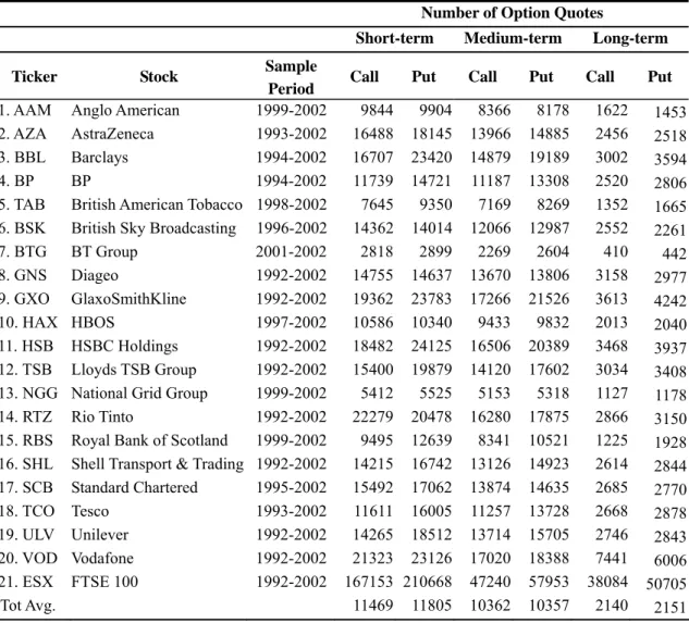
In this study we use daily settlement prices for 79 individual stock options and the FTSE 100 index option (ESX) traded on the London International Financial Futures and Options Exchange (LIFFE) as our research samples. The underlying stocks are traded on the London Stock Exchange (LSE). Individual stock options are American style, while the FTSE 100 index (ESX) option is European. The primary options data are obtained from the LIFFE database, and the corresponding stock prices and index data are from the DataStream database. The 3-month Treasury-bill rate is used as the proxy for the risk-free interest rate, which is also obtained from the DataStream database. The overall sample period extends from March 13, 1992 through December 31, 2002. The 79 individual stock options are selected simply because their price data are most complete for the whole sample period. However, the sample period for each of the 79 individual equity options varies with each other according to the availability of its price data. The sample period for each individual equity options is shown in Table 1.

Although we conduct empirical examinations for the 79 individual stock option contracts, here we only report the empirical results for the twenty largest stocks in FTSE 100 index. We alternatively report the averages of 79 stocks for the purpose of saving space. We decided to include the largest stocks, as their stock options are likely to be more liquid than those options on other smaller-sized stocks.

According to the methodology of BKM described in the previous section, we only use OTM calls and puts to construct the risk-neutral skewness and kurtosis. As a result, for each date, t, the puts in the sample always have moneyness corresponding to K/S(t)<1, and calls have moneyness corresponding to K/S(t)>1. As very short maturity stock option quotes may not be active, options with remaining days to expiration less than 9 days were discarded. Although options with longer-term maturity are illiquid compared to short-term options, we decided to incorporate them in this study to increase the degrees of freedom. To examine hypothesis across maturities, we group the sample options into three categories. If an OTM option has remaining days to expiration between 9 and 120 days, it is grouped in the short-term option category, if the remaining days to expiration falls between 121 and 240 days, the option is grouped in the medium-term category, and if the remaining days to expiration over 240 days, the option is grouped in the long-term category. Although arbitrary, this grouping criterion is convenient and should not be sensitive to our

empirical analysis.

Table 1 reports the number of observations, for the short-term, medium-term, and long-term OTM calls and puts, respectively, used in this study. As would be expected, the index has considerably more strikes quoted than individual stock options, with puts traded more actively than calls on average, except for the medium-term options. The number of ESX OTM puts exceeds the OTM calls by a substantial margin, possibly reflecting strong demand for downside insurance. In total, there are 1,780,231 option quotes (including 816,991 calls and 963,240 puts) included in the research sample.

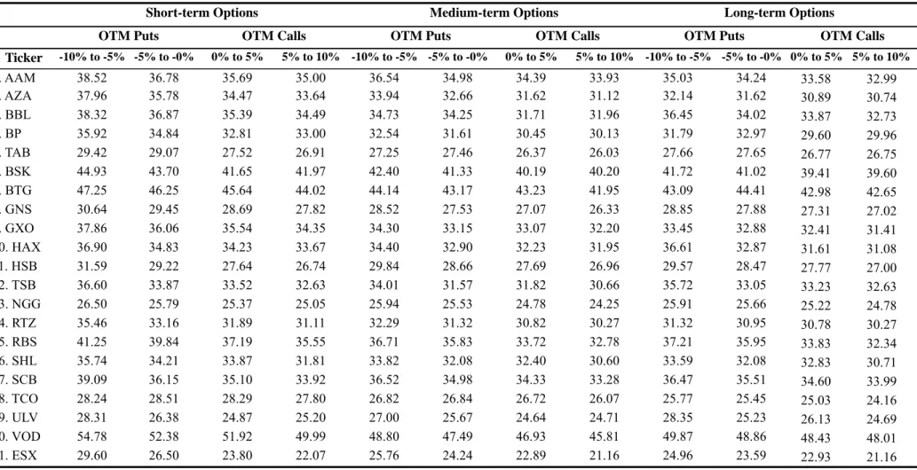
In Table 2 we report the summary of Black-Scholes implied volatility for options (calls and puts) on each stock and the FTSE 100 index, with short-term, medium-term, and long-term maturities. The implied volatilities of individual options are then averaged within each natural log of moneyness and maturity category. Among them, the OTM put options are used corresponding to the log-moneyness intervals [-10%, -5%] and [-5%, 0%], the OTM call options are used corresponding to the log-moneyness intervals [0%, 5%]

and [5%, 10%]. Without losing generality, we only report the results for the most recent year 2002, which corresponds to the period from January 1, 2002 through December 31, 2002. For other years the results are quite similar. Looking through the preliminary evidence, we observe that the average implied volatility for options with lower exercise price (OTM puts) is greater than that with higher exercise price (OTM calls). For example, in the case of short-term ESX options, the average implied volatility for OTM puts in the log-moneyness interval [-10%, -5%] is 29.60, while the average implied volatility for OTM calls in the log-moneyness interval [5%, 10%] is only 22.07%. In the case of medium-term and long-term ESX options, the average implied volatility decreases almost monotonously with the increases in the exercise price. This is also consistent for almost all individual stock options with all different times to maturity. These preliminary results also confirm the existence of the phenomenon of implied volatility skew in the LIFFE options market.

4. Empirical Examination

The above preliminary results indicate that the LIFFE equation options market exhibits a common phenomenon of implied volatility skew. We are now interested in the structures and characteristics embedded in this phenomenon. First of all, we need to quantify the slope of implied volatility curve and formally test whether the skew is statistically significant.

4.1 The slope of implied volatility skew

Hypothesis 1: For options with certain time to maturity, the slope of implied volatility curve across moneyness is negative.

To quantify the implied volatility skew, using options with certain time to maturity, we can measure the slope of implied volatility curve by the following regression model,

0 1

ln[STD y( )]_j =π +π ln( )y_j +ε_j j=1, 2, ," M (11) were y_j =K S_j/ is the moneyness of an option with the strike price K_j. There are M traded options for certain time to maturity at certain time. By regressing the logarithm of implied volatility on the logarithm of moneyness, the regression coefficient π₁, which represents the slope of implied volatility curve, can be the measure of the magnitude of implied volatility skew.

The model of equation (11) is estimated daily and across our sample of 79 stocks and the ESX, using a least-squares estimation (LSE). We then calculate the average of the estimated coefficients across time, and compute the t-statistics by dividing the average slope coefficient by its standard error. The model is estimated using only OTM puts and calls and conducted for short-term, medium-term, and long-term options, respectively.

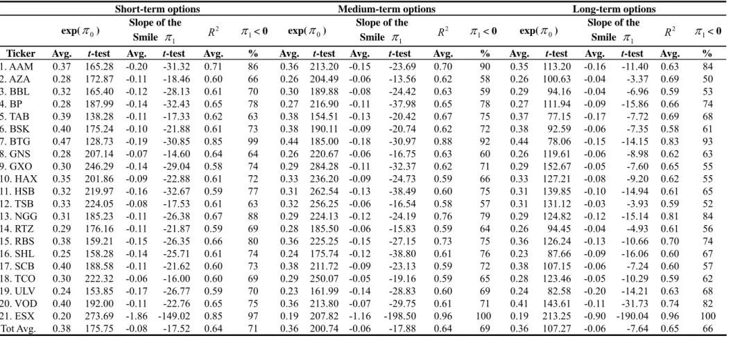
Table 3 reports the average of estimated slope of the implied volatility curve for each of the largest 20 stocks and the ESX options. The average slope of the 79 stocks is also reported. The intercept of the regression equation, π₀ has a particular meaning. Taking exponential function on π₀ results in exp(π₀) as

the estimated at-the-money (ATM) implied volatility. Consider the results for short-term options, the average ATM implied volatility for the ESX is about 20%, while the average ATM implied volatility for the 79 stocks is 38%, considerably greater than the market implied volatility. Concerning the estimate of π₁, there are several points to be made. First of all, on average, π₁ is negative for all of the individual stocks (ranging from -0.06 to -0.20) and the ESX (-1.86) options. The slopes are all statistically significant, and the R² of the regression ranges from 58% (for the GXO) to 85% (for the BGT) with the average of the 79 stocks being 64%. Second, the slope for the ESX is much steeper than that for the individual stocks. Compared to the short-term ESX slope of -1.86, the average slope over the 79 stock is only -0.08. Further compared to the results of BKM, we also find that the implied volatility slope of the ESX and individual stocks options which trade on the LIFFE, is flatter (less negative) than the S&P 100 index and the largest 30 individual stocks options trade on the CBOE.

Next, Table 3 also reports the statistic π₁<0, which is an indicator for the number of observation days in which the slope of the implied volatility curve is negative. This statistic ranges from 63% (for the TAB and TSB) to 99% (for the BGT) for short-term equity options. The statistic for the ESX is 97% and the average of the 79 stocks is 71%. This indicates that in most of the times during the sample period, the implied volatility curve is negatively skewed. Finally, we find the implied volatility curve for the ESX displays a smirk phenomenon, with respect to time to maturity, the long-term options is flatter than the medium-term and the short-term options, with short-term slope -1.86, medium-term slope -1.16, and long-term -0.90, respectively. For individual equity options, the slope is not unanimously flatter for the longer-term options than the short-term option. However, the average slope for short-term options is -0.08, and it is -0.06 for longer-term options. On average, this evidence is consistent with the empirical results of BKM and the theoretical inference of BFLW. We further formally test this hypothesis.

Hypothesis 2: The slope of implied volatility skew for short-term options is more negative than that for long-term options.

According to the model of BFLW, the longer maturity options induce the decrease of implied skewness and kurtosis. When maturity becomes infinite, the implied volatility skew will disappear, and the Black-Scholes formula will be valid. To formally test whether the implied volatility slopes for shorter-term options are steeper than that for longer-term options, for a certain day t, there are L options with different time to maturities traded, we thus combine the time-series data as well as the cross-sectional data to run the following regression model across our sample of 79 stocks and the ESX options

0 1

( , _tk) _{tk tk}

SLOPE t τ = Π + Π ⋅τ +ε ; k =1, 2, ," L; t=1, 2, ," T (12) where SLOPE denotes the slope of implied volatility curve obtained from the regression equation (11), τ_tk

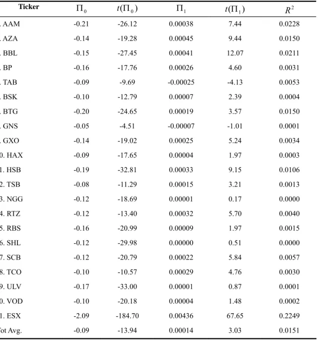
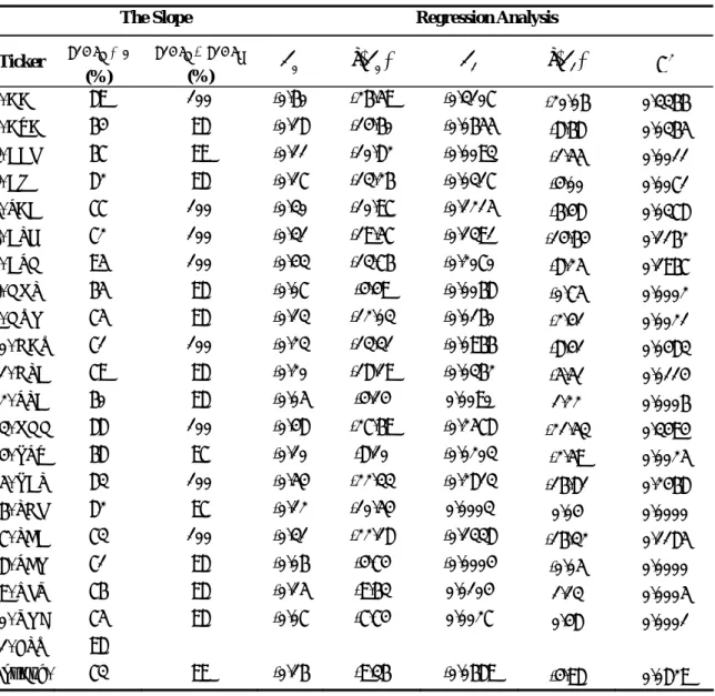
is the time to maturity of option k at time t. The model of equation (12) is estimated for each of the 79 stock and the ESX options using the OLS to estimate the regression coefficient Π₁. Table 4 reports the estimated coefficient for each of the 20 stocks and the ESX options. We also report the average estimate of the 79 stocks at the bottom row in the table. One can notice that the ESX option has the greatest value of Π₁, which is equal to 0.00436, compared to the average of 79 stock options, which is 0.00014. Overall the coefficients are mostly positive and statistically significant, with exceptions of the TAB (-0.00025, non-significant) and GNS (-0.00007, significant). In general, the evidence shows that increasing the time to maturity of options, flattens the implied volatility skew. However, the explanatory power is not high, with the ESX having the highest R² of 22.49%, compared to the average of 79 stocks of 1.51%. The result is also consistent with Duque and Lopes (2003) using LIFFE options for period from August 1990 to December 1991.

4.2 Implied volatility skew and risk-neutral skewness and kurtosis

Hypothesis 3: For options with certain time to maturity, the more negative the risk-neutral skewness, the steeper is the implied volatility slope. Furthermore, in the presence of the risk-neutral skewness, the more fat-tailed the risk-neutral distribution, the flatter is the implied volatility slope. However in the absence of the risk-neutral skewness, the more fat-tailed the risk-neutral distribution, the steeper is the implied volatility

slope.

According to BKM and BFLW which use the Gram-Charlier expansion to derive the option pricing model that allows the underlying distribution to deviate from log-normal, the Black-Scholes option implied volatility, STD t( , , )τ y for options with time to maturity of τ and moneyness of y, at time t, can be approximately expressed as a function of the risk-neutral skewness and kurtosis, which is:

( , , ) ( ) ( ) ( , ) ( ) ( , )

STD t τ y ≈α y +β y SKW t⋅ τ +θ y KUT t⋅ τ (13) where y = K/S is defined as the option moneyness, which is deterministic. The negative coefficient β( )y means that stocks with more negative skew have greater implied volatility at low levels of moneyness. The positive coefficient θ( )y specifies that stocks with greater kurtosis have higher implied volatility for both out of the money and in the money puts, resulting in an implied volatility smile phenomenon. In sum, with regard to the effect of higher-order moments on the shape of the implied volatility curve, the skewness represents the first-order effect relative to kurtosis, and a more negative skewness steepens the implied volatility curve. On the other hand, the kurtosis represents the second-order effect, and a greater kurtosis flattens the slope of the implied volatility curve in the presence of risk-neutral skewness. Whereas if we restrict on the effect of the skewness, the kurtosis will be a proxy for the skewness and will steepen the implied volatility curve.

Having quantified the implied volatility slope, we now can formally test the hypothesis 3. We first use the formulas (7), (8), (9), and (10) to estimate the price of the volatility contract, the cubic contract, and the quartic contract, respectively, and then use the formulas in (5) and (6) to estimate the risk-neutral skewness and kurtosis from OTM options. The risk-neutral moments are estimated daily, using the short-term, medium-term, and long-term options for the following regression model:

( , ) ( , ) ( , )

i i i i

SLOPE t τ = + ⋅α β SKW t τ θ+ ⋅KUT tτ +ε i=1, 2, ," N (14) where the series for the slope of implied volatility curve are the daily estimates of the coefficient π₁

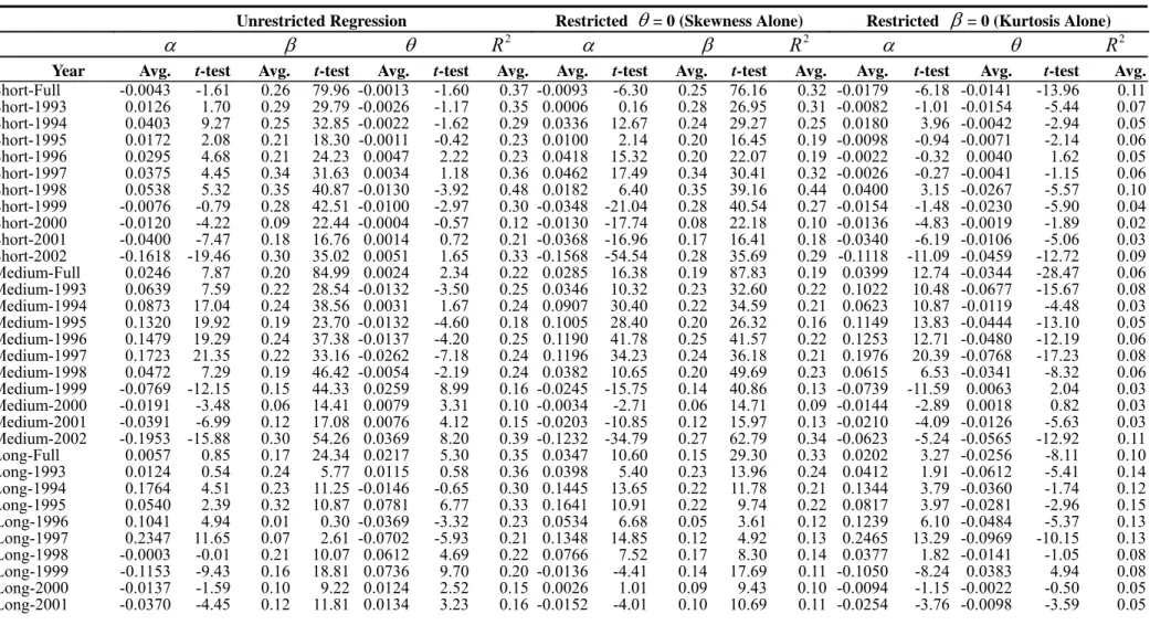
obtained from the regression model as in the equation (11). Having complied daily estimate of slopes and the corresponding moments for each of the 79 stocks, we can estimate the cross-sectional regression daily in the period from March 13, 1992 to December 31, 2002. We then average the estimated regression coefficients and the coefficients of determination, R², and report the results in Table 5. In order to check which variable play a dominant role in explaining the implied volatility skew, we conduct both the unrestricted multivariate regression of the equation (14), as well as the restricted univariate regressions (with only skewness or kurtosis as the explanatory variable separately). To assess the stability of the estimation, we also report the regression results for each year as a sub-period.

In the case of unrestricted multivariate regression, for all sub-periods in the sample period, regardless of the maturity structure of options, the average coefficients for risk-neutral skewness,β, are almost all significantly positive with the value ranging from 0.01 to 0.35. The evidence indicate that a more negatively skewed stock exhibits a steeper implied volatility curve, consistent with the first part of Hypothesis 3.

However, the results about estimated coefficients for risk-neutral kurtosis,θ , is mixed. For the short-term options, the full-period average of θ is -0.0013, with the t-statistic equal to -1.60, indicating non-significant statistically. For the medium-term and long-term options the full-period average coefficients of θ are 0.0024, and 0.0217 respectively, all positive and statistically significant. The average R² for the unrestricted regression is 37% for the short-term options, 22% for the medium-term options, and 35% for the long-term options. Although mixed, the results show that in general with the risk-neutral skewness in presence, the greater the risk-neutral kurtosis, the flattern is the slope of implied volatility. This is consistent with the second part of Hypothesis 3.

In the restricted regression cases we put the constraints, θ=0 or β=0, on the regression equation (14) to run a univariate regression model. Examining the restricted regressions, we can observe several interesting results. First of all, the full-period average R² for the short-term univariate regression with skewness alone is 32%, as compared to 11%, the case with kurtosis alone. In the cases of the medium-term and long-term univariate regression, it is 19% vs. 6%, and 33% vs. 10%, respectively. Obviously, the univariate regression

with skewness alone has a considerably greater average R² than that with kurtosis alone. Moving from the restricted regression with skewness alone to the unrestricted regression, the marginal contribution of the kurtosis to the explanatory power, R² is quite limited. This evidence support the hypothesis that the first-order effect on the implied volatility slopes is primarily driven by risk-neutral skewness. Further checking the sign and magnitude of the estimated coefficient, β, the sign remains unaltered, and the magnitude remains roughly the same, moving from the unrestricted regression to the restricted regression.

However the sign of coefficient on kurtosis, θ turns from mostly positive to almost all negative, and mostly statistically significant. This evidence is consistent with the third part of Hypothesis 3, claiming that in the absence of skewness, the kurtosis will come to play a proxy role for the skewness, steepening the implied volatility curve. In summary, the overall results are consistent with our conjectures, in the presence (absence) of negative the skewness, the kurtosis flattens (steepens) the implied volatility curve.

4.3 Implied volatility skew in individual stock and stock index options

Hypothesis 4: Individual stock option skew is determined by the index option skew and the idiosyncratic skew. On average, the individual stock option implied skewness is less negative than the index option implied skewness.

To consider the relation between the individual stock option implied skewness and the index option implied skewness, assume that τ-period return of individual stock i, R t_i( , )τ , follows a generating process of the single-factor model:

( , ) ( , ) ( , ) ( , ) ( , )

i i i m i

R t τ =a t τ +b t τ R t τ +ε τt (16) where R t_m( , )τ is the stock index return, a t_i( , )τ and b t_i( , )τ are scalars in the equation. The above return process is also well-defined under the risk-neutral measure, only some adjustments are needed for the parameters a t_i( , )τ and b t_i( , )τ . Assume that the unsystematic risk component ε τ_i( , )t has a zero mean, and it is independent of R t_m( , )τ for all t, then the relation between the individual stock option implied skewness, SKW t_i( , )τ and the index option implied skewness, SKW t_m( , )τ can be specified as:

( , ) ( , ) ( , ) ( , ) ( , )

i i m i

SKW t τ = A t τ ⋅SKW t τ +B t τ ⋅SKW t_ε τ (17) where SKW t_ε( , )τ is the skewness of the unsystematic risk component, ε, which is idiosyncratic to the individual stock. A t_i( , )τ and B t_i( , )τ are the scalars between zero and one. Note that the equation (17) is well-defined under either the physical or the risk-neutral measure, with certain adjustments for the scalars

( , )

A ti τ and B t_i( , )τ . This means that the individual risk-neutral skewness is a weighted combination of the risk-neutral market skewness and the idiosyncratic skewness. Under the condition that the idiosyncratic skewness is non-negative, or it does not significantly deviate from zero, as a result, SKW t_i( , )τ is greater than SKW t_m( , )τ , i.e., the individual stock option risk-neutral skewness is less negative than the risk-neutral skewness of the index option.

To check this, as reported in the first two columns of Table 6, for the largest 20 stocks, the averaged proportion of the total samples with negative skewness ranges from 72% to 95%. Across our sample of 79 stocks, the overall average proportion is 78%. While it is 98% for the ESX options, significantly higher than for the individual stocks. On average, the proportion that the individual skewness is greater (less negative) than the market skewness is 94%. In terms of magnitude, as shown in the last three columns of Table 7, the average skewness for the ESX options is -1.75, substantially more negatively skewed than any of the 20 stocks, as well as the overall average across the 79 stocks, which is -0.22. Incidentally, the average implied volatility of the ESX options is less than any of the individual stocks and the overall average, while the average of risk-neutral kurtosis for the ESX options is much higher than for individual stock options.

Next corresponding to the equation (17), we construct the following regression model using time-series data across different time to maturity, to examine the importance of market skew in explaining the individual stock skew.

0 1

( , ) ( , ) ( , )

i k m k i k

SKW tτ =λ λ+ ⋅SKW t τ +ε τt ; t=1, 2, ," T;k=1, 2, ," L (18) The testing hypothesis is that the regression coefficient, λ₁ is greater than zero and less than one. The regression results are shown in the middle part of Table 7.

The results are mixed, with only slightly more than one-half of the estimated coefficient λ₁ significantly positive, and the others significantly negative. Nonetheless, we notice that the coefficients of determination are all small, with only three stocks having R² great than 10% (AAM, TAB, and BTG). One possible interpretation of this result is that the idiosyncratic skew is more important than that of the market skew in determining the risk-neutral individual skew. Alternatively, the idiosyncratic skew may be directionally offsetting the negative market skew.

Similarly, recognizing the relationship between the slope of implied volatility skew and the risk-neutral skewness, it follows that the implied volatility curves are less negatively sloped for individual stock options than for stock index options. As shown in the first two columns of Table 8, we can observe that the slopes for implied volatility curve are mostly negative, and the slopes for individual stock are almost all less negative than the slope for the index options. This evidence is quite consistent with our conjecture. Incidentally, we also consider the following regression model to test whether the slope of implied volatility curve is determined by the market slope.

0 1

( , ) ( , ) ( , )

i k m k i k

SLOPE t τ =η η+ ⋅SLOPE tτ +ε τt ;t=1, 2, ," T;k=1, 2, ," L (19) As shown in Table 7, the regression coefficients, η₁ are mostly negative and about two-third of the 20 stocks have the estimate statistically significant. Overall average of the estimated coefficient is -0.0689, which is significant. For some stocks, the R² is as high as 0.3494, while for others it is as low as 0.0000, varying across the sample stock quite drastically. The average R² is 0.0829, a moderate level. The results indicate that the slope of implied volatility skew for individual stock options is negatively correlated with that for the stock index options. These results seem to contradict the BKM hypothesis.

5. Conclusion

In this article, we empirically examine the phenomenon of implied volatility skew in LIFFE equity options. We investigate the structure and characteristic of the risk-neutral skewness and kurtosis which is in relation to implied volatility skew, using prices of 79 individual stock options and the FTSE 100 index options, with the sample period extending from March 13, 1992 through December 31, 2002. Only out-of-the-money options are used for calculating the risk-neutral moments and testing the hypotheses. In total, there are 816,991 call prices and 963,240 put prices used as research sample in this study. Based on the model of BKM, we test several interesting hypotheses and obtain sometimes contrasting empirical results.

First of all, the slope of implied volatility curve is significantly negative for both individual stock options and stock index options. And the implied volatility skew can be described by risk-neutral skewness and kurtosis to some extent, where the risk-neutral skewness dominates the risk-neutral kurtosis in explaining the effect, leaving the risk-neutral kurtosis to be the second-order. Furthermore, the slope of implied volatility skew increases as the time-to-maturity of options increases, meaning the negativity of the slope becomes less for longer-term options, which is consistent with the model of BFLW. Moreover, the implied volatility skew for individual stock options is less severe than that of the stock index options. And the idiosyncratic component dominates the market component in determining the individual stock risk-neutral skewness. Finally, as we relate the risk-neutral skewness and kurtosis to the physical ones, the risk-aversion parameter comes to play its significant role. The empirical estimation for the risk-aversion parameter is significantly positive and quite consistent in quantity confirming the stable relationship between the physical and the risk-neutral moments implied in option prices.

References

Ait-Sahalia, Y., and A. Lo, 1998,”Nonparametric Estimation of State-Price Densities Implicit in Financial Prices”, Journal of Finance 53, No. 2, 499-548.

Backus, D., S. Foresi, K. Lai, and L. Wu, 1997, “Accounting for Biases in Black-Scholes”, mimeo, New