最適促銷組合之策略 – 建構於馬可夫轉換模型

國

立

交

通

大

學

經營管理研究所

碩

士

論

文

最適促銷組合之策略 – 建構於馬可夫轉換模型

Optimal Sales Promotion Strategy

- Markov Switching Approach

研 究 生：黃俊諺

指導教授：唐瓔璋 教授

最適促銷組合之策略 – 建構於馬可夫轉換模型

Optimal Sales Promotion Strategy

- Markov Switching Approach

研究生：黃俊諺

Student：Jiun Yan Hang

指導教授：唐瓔璋

Advisor： Edwin Tang

國立交通大學

經營管理研究所

碩士論文

A Thesis

Submitted to Institute of Business and Management

College of Management

National Chiao Tung University

in Partial Fulfillment of the Requirements

for the Degree of

Master of Business Administration

June 2008

Taipei, Taiwan, Republic of China

中華民國 九十七 年 六 月

i

最適促銷組合之策略 – 建構於馬可夫轉換模型

學生:黃俊諺

指導教授:唐瓔璋 博士

國立交通大學經營管理﹙研究所﹚碩士班

摘要

本論文主旨在於研究，如何在競爭激烈的快速流通產品產業中建立促銷組合之最佳 策略，在文中，我們利用品類管理的觀點分別檢視不同的品類、包裝以及通路，並且使 用馬可夫轉換模型將銷售分為促銷期間以及非促銷期間衡量以衡量跨期促銷投入的效 果。首先我們利用模型決定衡量過去促銷投入的標準，進而以對過去促銷投入的評鑑作 為未來預算投入的準則，解決品牌經理或產品經理過去以直覺、過去經驗、或隨機決定 預算分配的困境；我們利用馬可夫轉換模型所建立的假設，尋求未來進行促銷投入時， 促銷期間與非促銷期間的比例，以及其間隔時間的長短、促銷次數等，；最後我們利模 型所顯現的結果歸納出未來廠商進行策略決策時的準則。 我們使用目前世界最大的食品公司過去 39 個月的銷售以及促銷投入的資料，進行 行銷組合之最佳策略之研究。數據結果顯示，過去的促銷投入的次數過多，且並未在刺 激銷售上有明顯的效果；此外我們發現在擬定促銷方案時，應當考量產品銷售量的多寡， 使用不同的促銷型式。最終的目的在於提供品牌經理以及產品經理一個具理論基礎的解 決方案。 關鍵字: 品類管理、馬可夫轉換模型、促銷組合

ii

Optimal Sales Promotion Strategy

- Markov Switching Approach

Student：Jiun Yan Huang Advisors：Dr. Edwin Tang

Department﹙Institute﹚of Business and Management

National Chiao Tung University

Abstract

This paper investigates the optimal sales promotional strategy for the fiercely competitive FMCG (Fast Moving Consuming Goods) industry. We propose a Markov Switching Autoregressive model that incorporates AR(1) retailing demand process to capture nonlinear structure among promotional budget allocation, evaluation of promotion performance, and optimal promotion frequency within a given time span. The past promotion investment is evaluated first by comparing the changes in promotional budget allocation. We then apply Markov switching feedback rules to figure out the proper length of equilibrium state with and/or without promotion. Finally, effective decision rules on magnitude, duration, and frequency of promotional strategy are induced. We apply three product categories with 39 months time-series data from a multinational packaged food company. The result shows that most past decisions on promotional budget allocation are non-optimal – most promotion investments were either extended too long or allocated too low in stimulating sales. Implications for the brand- or category- manager in removing those non-optimal promotional policies are suggested.

iii

Content

摘要 ... I ABSTRACT ... II CONTENT ... II LIST OF TABLE ... IV LIST OF FIGURE ... IV 1. INTRODUCTION ... 1 2. REVIEW ... 6 2.1CATEGORY MANAGEMENT ... 6 2.2SALES PROMOTION ... 9

2.3MARKOV SWITCHING AR(1)TIMES SERIES MODEL ... 12

3. MODELING ...14

3.1RESEARCH OBJECTIVES... 14

3.2DATA ... 14

3.3LINEAR REGRESSION ... 18

3.4OPTIMAL SALES PROMOTION –MARKOV SWITCHING MODEL ... 19

4. ANALYSIS ...26

4.1LINEAR REGRESSION MODEL ANALYSIS ... 26

4.2MARKOV SWITCHING MODEL ANALYSIS ... 27

5. CONCLUSION...30

iv

List of Table

Table 3-1 Classification of promotion expenditure ... 15

Table 3-2 scanner data table ... 17

Table 3-3 Notations and Symbols ... 21

Table 4-1 Result of the linear regression ... 26

Table 4-2 Result of the moderation effect ... 26

Table 4-3 Summary of θij ... 28

Table 5-1 Comparison table between average sales and θ ... 31

Table 5-2 Comparison table between promotion expenditure and θ ... 32

List of Figure

Figure 1-1 Research Framework under regression model ... 2

Figure 1-2 Decision making framework under Markov Switching model ... 3

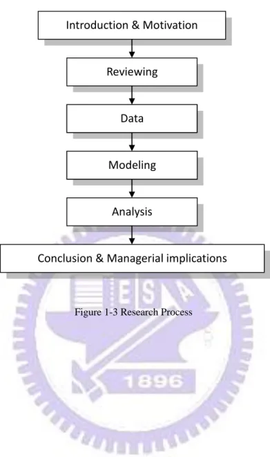
Figure 1-3 Research Process... 5

1

1. INTRODUCTION

A fundamental change is taking place in the FMCG (Fast Moving Consuming Goods) industry as retailers and manufacturers begin to embrace a process called category management (CM) (Suman, Murali, & Rockney, 2001). And so is to the manufacturers and development. Not too many years ago, manufacturers were the leaders of the marketplace, and retailers were their distribution arms. Manufacturers knew marketplace well, and retailers were content to rely on their marketing wisdom. But now consumers have changed. Faced with so many shopping options, and recognizing the intense price competition that exists among retailers, today‟s shopper is more likely than ever to cherry-pick among stores – and among brands. While the market is getting mature and even the decline period of the product life cycle, manufacturers faced the problem improving their economic performance and what is the benefit as they invest huge on pricing, promotion, and merchandising activities.

In our study, we use the latest data of a multinational packaged food company, which is a global market leader in many product lines, including milk, chocolate, confectionery, bottled water, coffee, ice cream, food seasoning and pet foods, and the data had witnessed many innovative promotion activities in the recent past. We look into two categories, bouillons and seasonings, with three kinds of packages and split up into sales promotion.

Promotion has, for a long time, been one of the topics most frequently discussed by both marketing practitioners and researchers. It is still worth debating. Promotion decision under category management involves three decision aspects: promotion depth (i.e., how much money should they invest), promotion frequency (i.e., how often a store should offer a discounted price), and promotion extent (i.e., how many products in the category should be promoted). So far, promotion has been done in varied ways, including coupons, direct mails, B2B, B2C, on-pack policy, events and so on, and we call it sales promotion.

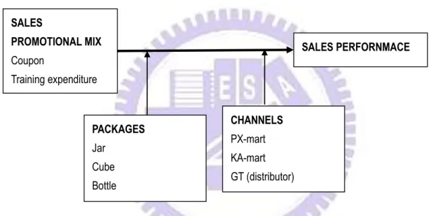
So we consider the promotion decision among varied channels, different product categories and dissimilar kinds of sales promotion. In the first part of analysis, we use a linear regression model to test our research framework shown in figure 1. We suppose categories, packages and channels have a moderate effect on sales promotion. However, we expect that it

2 SALES PERFORNMACE SALES PROMOTIONAL MIX Coupon Training expenditure Display expenditure CHANNELS PX-mart KA-mart GT (distributor) PACKAGES Jar Cube Bottle

Figure 1-1 Research Framework under regression model

will not be significant. Numerous factors were responsible for such a phenomenon. One of the reasons being that the market being sluggish, companies were trying to increase market share in stagnant to declining (volume terms) market in order to retain consumers, to encourage switching, to induce trials and liquidate excessive inventories. Another reason possible was that with the presence of so many brands the competition had increased severally leading to fight for market share and shelf space. If a significant impact didn‟t exist, it result in some problem that brand manager would get confused with the future promotion input.

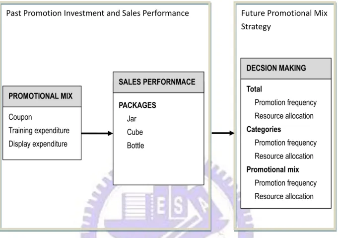
In order to provide a better solution to the manufactures, in the second part of analysis, we use a Markov Switching AR(1) times series Model, which could capture a spike-shaped response of demand to promotion by switching two promotion states and analyze the optimal promotion frequency. Based on the model and research framework shown in figure 2, we want to develop a model to help brand manager make an optimal promotion frequency decision under a budget constraint.

3

Future Promotional Mix Strategy Coupon Training expenditure Display expenditure PACKAGES Jar Cube Bottle SALES PERFORNMACE

PROMOTIONAL MIX Total

Promotion frequency Resource allocation Categories Promotion frequency Resource allocation Promotional mix Promotion frequency Resource allocation DECSION MAKING

Figure 1-2 Decision making framework under Markov Switching model Past Promotion Investment and Sales Performance

To sum up, this study can provide the most important guidance on the following issues:

 Considering the issues at the same time, sales promotion, categories, and packages :

In our study, we provide a total solution to the manufactures by considering categories, packages, and sales promotion together, which is the difficult position they deal with all day long.

 Evaluating promotion performance :

Manufacturers are always confused with the effect of promotion when they faced so many product categories at the same time. Sometimes the effect of promotion may happen at next period according to the inventory of household (Chakravarthi, Scott, & Subrata, 1996). Understanding how well the different type of promotion works in the cross-category should provide a benchmark for assessing the performance of each category‟s promotions.

4  Resource allocation

At each decision-making period, brand manager has to allocate his own resources and limited budget on the categories. They will not only dependent on their experiences but the promotion-responsiveness of the category before. However, the promotion-responsiveness would be ignored by the brand manager because of the complexity and they just take a quick glance on the scanner panel data. By using the Markov Switching Model they can easily know the promotions work or not and move further beyond budget allocation problem.

We begin by reviewing relevant literature about sales promotion, with discussion of the depth and the frequency of promotion, and the Markov Switching AR(1) time series Model, the most important parts of this study, to introduce the whole concept of this study. Next, we develop a framework for understanding different types of promotion in distinct categories, and use it to generate hypotheses. We then describe our measurement and analysis methodology and present our results. We conclude with a discussion of managerial implications and opportunities for further research. And the research process is as below:

5

Introduction & Motivation

Reviewing

Modeling

Data

Analysis

Conclusion & Managerial implications Data

Modeling

6

2. REVIEW

2.1 Category Management

In 1995, the Category Management Subcommittee of the ECR Best Practice Operating Committee and the Partnering Group Inc. published an important study: Category

Management Report: Enhancing Consumer Value in the Grocery Industry. This report is

basically the how-to of CM and lays out eight critical steps that the necessary for a proper implementation of CM by a retailer. However, this study is from the aspect of the manufacturer. For manufacturer, category management is an ongoing, dynamic process that involves managing categories as separate businesses, each with its own pricing and profit/loss responsibilities. The manufacturer can undertake this new selling/marketing approach most successfully by focusing on five stages. They include: (Nielsen marketing research, 1992)

I. Reviewing the category

The first stage, reviewing the category, requires that a manufacturer gather and integrate a broad range of internal and external data to create a national overview of the category. Essential pieces of information include the category‟s unit and dollar volume and growth rates, both on a national basis and by retail trade channel; the level of advertising and promotional activity within the category; and the number of new products introduced into the category during the last year. The manufacturer also should examine national household purchasing patterns, including how many households buy products from the category, where they shop and how much they spend. It‟s also important for the manufacturer to chart the performance of its brands versus those of competitors at the national, market and retail-account levels.

II. Targeting consumers

This stage involves three steps: (1) Building a demographic profile of the typical buyer, both for the category and for a specific brand. The profile would include information such as income level, family size and age. It also would indicate whether the typical buyer purchased a lot or a little, where the purchases usually occurred, whether

7

the typical buyer was price-sensitive, and whether he was likely to use coupons. (2) Identifying and evaluating target groups. This step involves analyzing general information about the lifestyles of target consumers. What products do they buy? What stores d they shop at? That leisure activities do they pursue? This information can yield a deeper understanding of the needs of target customers. It also can help a manufacturer identify cross-merchandising opportunities and can provide useful knowledge for the development of advertising aimed at target consumers. (3) Planning promotion and media strategies. By examining data on consumer media preferences, the manufacturer can select the appropriate advertising vehicles such as television, radio, magazines and newspapers, for reaching target consumers.

III. Planning merchandising

The third stage of category management, planning merchandising, involves developing a detailed strategy by retail account for product mix, pricing, promotion, and shelf-space allocation within a category. In examining product mix, a manufacturer can use software applications to determine which of its brands a particular retailer does not carry and which of these have strong volume potential for both the retailer and the manufacturer. These applications also enable a manufacturer to recommend an optimum product mix by projecting the volume and profit gains a retailer would realize by adding such items. By making such recommendations, a manufacturer can demonstrate its category knowledge to the retailer. When trying to determine appropriate pricing and promotion strategies for a category, a manufacturer must recognize that retailers design specific promotional programs for each store or cluster of stores, and that the manufacturer‟s brand or brands are only part of the entire category. Both the retailer and manufacturer must focus on the category as a whole to execute mutually beneficial pricing and promotional strategies.

Our study involves this step by looking forward to the varied channels and analyzing the impact of the consumer promotion, which indicates a demo to the retailer, cross the categories.

8 IV. Implementing strategy

At this point, the manufacturer‟s team sales leader makes his presentation to the category buyer at the retail account for which the strategy was devised. Using information gleaned during the first three stages of the category management process, the team sales leader provides an overview of the category, his brands and consumer purchasing patterns. In discussing promotions, the manufacturer should note opportunities to tie together promotions across categories, and to take maximum advantage of special allowances provided by the manufacturer. Leading-edge manufacturers have begun to sign one-year contracts stipulating the amount in special allowances a retailer will receive over a 12-month period, with the understanding that the manufacturer and retailer will try to tie their promotions together. Implementing strategy isn‟t confined to one presentation to a retailer buyer. It‟s a long process that requires a continuing dialogue between the manufacturer and the retailer. After implementing merchandising and marketing strategies for a category the manufacturer next must evaluate their impact.

This study involves this step by discussing the promotional pix cross categories and channels. Furthermore we could provide a guide to the optimal promotion strategy of the manufacturer.

V. Evaluating results

This fifth stage of category management is as critical to the process as pedals are to a bicycle. That‟s because it involves questions, answers and decisions that keep the circular process flowing naturally back into its first stage, reviewing the category. This knowledge can help manufacturer‟s sales managers and brand managers identify new opportunities and unforeseen challenges in the marketplace. They then must decide if and how to modify their strategies. These decisions require managers to review their category once again, providing the link that makes category management a dynamic, ongoing process.

9

promotion which cover the most critical step of the category management.

Most empirical research only discusses one or two step of the process. Fader and Lodish (1990) examine various structural characteristics of categories and relate them to the frequency and types of promotions offered by retailers and manufacturers and it covers the first and third step of the process. Dhar, Hoch, and Kumar (2001) relate the variability in category performance across retailers to category characteristics and retailer pricing, promotion, and merchandising strategy, while controlling for the level of manufacturer support and it covers only the third step of the process. Our study apparently would cover three step of the process, the 3rd, 4th, and 5th steps, providing a more comprehensive discussion than ever before.

2.2 Sales Promotion

In many industries, sales promotions represent a significant percentage of the marketing mix budget. Nondurable goods manufacturers now even spend more money on sales promotion than on advertising. Kotler (2006) defines sales promotion as: “Sales promotion consists of a diverse collection of incentive tools, mostly short-term designed to stimulate quicker and/or greater purchase of particular products/services by consumers or the trade.” Roger Strang (2006) has given a more simplistic definition i.e. “sales promotions are short-term incentives to encourage purchase or sales of a product or service.”Sale promotion in our study primarily indicates coupon and on-pack policy. The effectiveness of a sales promotion can be examined by decomposing the sales “bump” during the promotion period into sales increase due to brand switching, purchase time acceleration, and stockpiling (Gupta Sunil 1988). According to our data, we classify several sales promotion tools as below:  Coupon

It is well recognized in the marketing literature that coupons have immediately impacts on sales. Most of them are a short-tem promotion not to only accelerate consumer‟s purchases but maximize the total sales (Neslin, Quelch, & Henderson, 1985). Previous research has shown that brand sales increase shortly after coupons are distributed (Iron, Little, & Klein 1983, Klein 1981, Neslin, Henderson, & Quelch 1985),

10

but these short-term gains appear to be attributed mainly to consumers who switch temporarily from the other brands to the coupon-promoted brands (Johnson, 1984). From the manufacturer‟s perspective, the profitability of the couponing operation is a function of both the incremental sales generated by the coupon and the number of coupons redeemed (Leone and Srinivasan, 1996). Ronald and James (1978) used a regression model to show that purchases quantities of orange juice were larger when coupons were used in the purchases.

 Training Expenditure

Training Expenditure in our study indicates the expenditure to salesman or promoters. Salesman or promoters can deliver the latest information from the market to the manufacturers, and it is very useful while manufacturers doesn‟t know marketplace well. They also have a big influence on the selling. However, turnover of salespeople possessing high transaction specific asset is costly to the firm because it is difficult for a firm to hire salespeople with comparable skill. When salespeople are hired who do not possess these skills, the firm suffers an opportunity loss and a direct cost as salespeople are trained about the unique aspects of the firm (Ganesan, Weitz, Barton, & John, 1993). So the Training Expenditure is a good tool for manufacturers to retain their sales productivity. The higher expenditure to salesman or promoters, the more they can do. An excellent promoter has higher perceptions of the importance of promotions than non-excellent promoting retailers and they follow up by spending more on the total promotion budget (Friestad and Wright, 1994).

 Display expenditure

In this study, display expenditure mainly indicates event, display on the shelf, and road-show held in the retail stores. Such display and feature expenditure have strong effects on sales item. The effect of display and feature expenditure was found by Woodside and Waddle (1975), Blattberg and Wisniewski (1987), and Kumar and Leone (1988). Bemmaor and Mouchoux (1991), Bolton (1989), and Kumar and Leone (1988) also confirm the effect. We recognized the display expenditure is getting important but how it works? Retailers are the vehicles for pass-through of promotional money to

11

consumers. It is important to recognize that most brands receive far less than 100% pass-through.(Chevalier and Churchman 1976, Curhan and Kopp 1986, Walter 1989, Blattberg and Neslin 1990)

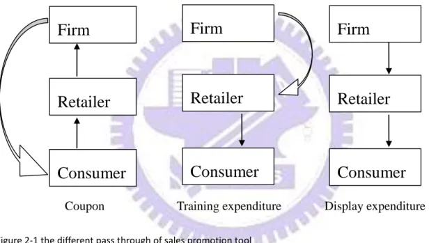
Each sales promotion tool has its own way passing the effort to the consumer. Coupon, sent to the consumer, would stimulate the sales in the retailers, and result in the expenditure on coupon from retailers. Training expenditure is spent directly to the retailers and retains their sales productivity to push consumer purchasing. Firm spent display expenditure on shelf space, displays, or road show in the retailer store and make their product exposure more to let consumer purchase.

Figure 2-1 the different pass through of sales promotion tool

However, not only the types of promotion act different influences on sales. Some findings indicate that the frequency of promotion changes the consumer‟s reference price. Those findings offer an explanation for the loss of brand equity when brands are heavily promoted. A lower consumer reference price reduces the premium that can be charged for a brand in the marketplace, which result in less “equity.” The effect of deal frequency on consumer‟s reference price was found by Lattin and Bucklin (1989), Kalwani and Yim (1992), Mayhew and Winer (1992). The greater the frequency of deals, also the lower the height of the deal spike. This result is likely to be caused by (1) consumer expectations about the frequency of deals and (2) changes in the consumer‟s reference price. The empirical result

Firm

Consumer

Retailer

Firm

Consumer

Retailer

Firm

Consumer

Retailer

12

was documented by Bolton (1989), Raju (1992), and indirectly through the preceding generalization (3), which, in combination with Winer (1986), links reference price to purchases behavior. So the promotion frequency is a very important part of the sales promotion strategy. It affects the sales but has a negative effect on the perceived brand quality, and brand image.

On the other side, how would it affect the brand equity if we do long-term promotion? Advocates of advertising (e.g., advertising agency) often argue that promotions are detrimental to the long-term health of brands. Early research seemed to confirm this long-term negative effect (e.g., Dodson et al. 1978 and Strang 1975) but later studies began question this result (e.g., Johnson 1984). “How many times” and “how long” are two major problems faced by brand or product managers. Furthermore, they might have a budget constraint so that it would very difficult to determine the optimal frequency and optimal period of a promotion campaign. All above are the key of long-term sales promotion plan.

2.3 Markov Switching AR (1) Times Series Model

Hisashi, and John (2006) use the Markov switching model to describe how promotion influences sales at the retailer. A Markov switching time series model is an established approach in econometrics and is considered to be able to properly describe time series data that might shift from one regime to another according to unobserved random variables (Hamilton, 1990, 1994, 1996). Achabal, McIntyer, and Smith (1990) developed a closed-form analytical response model that can determine the periodic promotion plan of both discount depth and frequency, including the impact of seasonal and inventory effects. Rao (1991) modeled the equilibrium of promotion depth and frequency by applying a multi-stage game-the-oretic model, and analyzed the competition between national and store brands. The experimental study by Kalwani and Yim (1992) investigated the impact of the depth and frequency of price discount promotion on customers‟ expected price formulation and brand-choice behavior. Assuming that demand follows a discrete Markov process and that market share changes over time due to advertising, Bronnenberg (1998) studied the optimal advertising planning decision under a budget constraint. Before proceeding, it is useful to

13

describe the types of promotions considered in this article. For example, one often observes that sales suddenly soar on the day of a special promotion. Marketing research (for example, Blattberg and Neslin, 1990, pp. 344–345) reports that the time series plot of actual sales has „„spikes‟‟ due to promotion. While traditional market response models, such as the linear or multiplicative methods, have difficulty in expressing an impulsive increase in demand caused by promotion, a Markov switching model can. They analyzed the optimal promotion depth and frequency under a supply chain framework, when the retailer wants to maximize expected revenue and the supplier tries to minimize expected inventory cost.

We not only base on the Markov Switching Model to have the optimal promotion depth and frequency but look into these decisions by packages, categories, channels, and types of promotion. According to the Hisashi, and John research in 2006, they treat θ as promotion frequency and as they proved θ∗ represent the optimal promotion frequency, which is related to the sales of non-promotion state and promotion state1 and the unit promotion cost. In our study, we consider θ∗ as a measurement of evaluating manufacture‟s promotion performance and also a unit of the budget allocation.

1

θ∗=_2kμp

2 μ2− μ1 , μ2 are the sales of promotion state, μ1 are the sales of non-promotion state, and k

14

3. MODELING

3.1 Research Objectives

This study intends to build up a tool, which guide brand managers modifying their sales promotion strategy.

First, we use linear regression model to test the significance of sales promotion and the moderate effect of categories, packages, and outlets. We assume that linear regression couldn‟t explain the variation of sales performance via sales promotion and neither could the moderation effect. Second, we provide another measurement using Markov Chain Switching Model to evaluate performance of sales promotion with time series scanner data. We defined promotion-state period and non-promotion-state period to see what is the difference. We find out the optimal promotion frequency by θ for a given period. Third, based on the results we could get θ, which indicate the effect of promotion and we use θ as the proportion to allocate the limited budget. A brand manager usually handles two more product categories with flavors or packages so that how to efficiently use their own resources becomes a tough problem.

3.2 Data

Our data include a time series sales of varied outlets, stable list price, and investment to the sales promotion.

 Outlet

We can see three outlets in the panel data. One is PX mart, used to only sell to the army before, but now PX mart has over 700 retail stores in Taiwan and provides over 6000 brands on the shelves. PX mart is a special outlet that is probably unique in the world. When the PX mart first established, it‟s just like a VIP club and in the store whole product is discounted about 20% of the list price. Around 10 years ago, PX mart turned to an opening store and was still with the high discount rate so PX mart left the consumer

15

a “the cheapest” image. Now in Taiwan, PX mart is the most widely distributive retail stores in FMCG industry.

Second is hypermarket, including Carrefour, a French international hypermarket chain with a global network of outlets, and RT-MART, a Taiwan corporation builded in 1996. In commerce, a hypermarket is a superstore which combines a supermarket and a department store. The result is a very large retail facility which carries an enormous range of products under one roof, including full lines of groceries and general merchandise. When they are planned, constructed, and executed correctly, a consumer can ideally satisfy all of their routine weekly shopping needs in one trip. Hypermarkets, like other big-box stores, typically have business models focusing on high-volume, low-margin sales. Because of their large footprints , a typical Carrefour 19,500 m² (210,000 square feet), and the need for many shoppers to carry large quantities of goods, many hypermarkets choose suburban or out-of-town locations that are easily accessible by automobile.

Three is distributor. Distributors make profit by taking orders from the manufacturer and selling them to the retailers. It‟s far different from the two kinds of outlets we mentioned above which could sell the product on the shelves in their own stores.

 Investment of sales promotion

We have a variety of promotion tools, including online e-commerce, CI, trade-promotion, POSM, sample, events, and coupons. As our reviewing, we classify each promotion tool into the different types of promotion. And the classifications are as the table below:

Table 3-1 Classification of promotion expenditure

16  Coupons expenditure

Coupon is a ticket or document that can be exchanged for a financial discount or rebate when purchasing a product. And it includes the on-pack promotion in our study.

Coupon

 CI

CI is an investment of corporate communication between manufacturers and outlets in order to transfer the product information helping salespeople or retailers know more about the categories

 Sample expenditure

Sample means brand manager will give salespeople and promoter samples of the product to let them taste.

Training expenditure

 POSM expenditure

POSM refers to the layout on the shelf, including posters, stand, and any other decoration, making the categories strikingly in the store.

 Event expenditure

Event expenditure is for holding display and road show for the categories in the stores.

 CCD expenditure

It refers to the expenditure to increase the shelf space and the trade promotion money passed through to the consumer.

Display Expenditure

The total promotion spent on Bouillons and Seasoning were NT$ 3276.22 thousands and NT$ 2177.47 thousands. The Coupon spent on Bouillons and Seasoning were NT$ 990 thousands and NT$ 472 thousands. The display expenditure spent on Bouillons and Seasoning were NT$ 202.5 thousands and NT$ 382 thousands. The display expenditure spent on Bouillons and Seasoning were NT$ 2083.72 thousands and NT$ 1323.47 thousands. Obviously, they spent more on the Bouillons.

17

Price in our study, we treat it as a given exogenous variable. Because we are from the aspect of a brand manager which only take charge of the sales promotion strategy meanwhile the salespeople take charge of price discount or price cut of the outlets. And the categories we discuss have also rarely been price cut or price discounted in the retail stores. So we put a given list price into our model in order to rustically measure the performance of sales promotion regardless of the selling price.

 Sales of categories

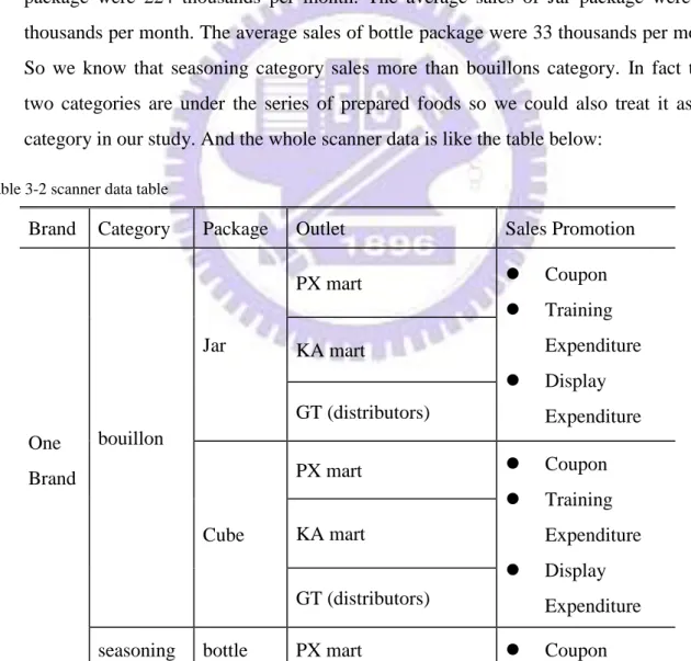
We examine two categories, bouillon and seasoning, with 39 months sales number and we will check the time series data by AR(1) process. The average sales of bottle package were 224 thousands per month. The average sales of Jar package were 156 thousands per month. The average sales of bottle package were 33 thousands per month. So we know that seasoning category sales more than bouillons category. In fact these two categories are under the series of prepared foods so we could also treat it as one category in our study. And the whole scanner data is like the table below:

Table 3-2 scanner data table

Brand Category Package Outlet Sales Promotion

One Brand bouillon Jar PX mart  Coupon  Training Expenditure  Display Expenditure KA mart GT (distributors) Cube PX mart  Coupon  Training Expenditure  Display Expenditure KA mart GT (distributors)

18 KA mart  Training Expenditure  Display Expenditure GT (distributors)

3.3 Linear Regression

In our first part of discussion, we use linear regression model to test significant influence of sales promotion on sales performance and the interactive impact of the sales promotion and moderator, outlets, packages, and categories.

In the beginning, we use simple linear regression to test the performance of sales promotion. The dependent variable is the sales revenue and the independent variable is the amount of promotion expenditure. We find out that the sales revenue has autocorrelation with the former period, following AR(1) process therefore we put a sales revenue of former period as a controlled variable into each regression model. We use the AUTOREG procedure in SAS language which enables us to estimate and predict of linear regression models with autoregressive errors and to test linear hypotheses and estimate. The regression model and the definition of each variable are as below:

𝐘_{𝐭𝐢𝐣𝐤}= 𝛃𝟎+ 𝛃𝟏 𝐘𝐭−𝟏𝐢𝐣𝐤+ 𝛃𝟐𝐗𝟏𝐢+ 𝛆𝓲𝟏 𝛆𝓲𝟏~𝓲𝓲𝓭

𝐘_{𝐭𝐢𝐣𝐤} represents the sales revenue in period t

𝐘_{𝐭−𝟏𝐢𝐣𝐤} represents the sales revenue in period t-1 𝐗𝟏𝐢 represents the amount of promotion expenditure

∀ i = 1, 2, 3, 4

1 represents sum of all sales promotion, 2 represents coupon, 3 represents training expediture, 4 represents display expenditure ∀ j = 1, 2, 3

1 represents Jar, 2 represents Cube, 4 represents bottle ∀ k = 1, 2, 3, 4

19

And then, we test the moderation effect including categories, packages, and outlets. The regression model is as below:

𝐘_{𝐭𝐢𝐣𝐤} = 𝛃_𝟎+ 𝛃_𝟏 𝐘_{𝐭−𝟏𝐢𝐣𝐤}+ 𝛃_𝟐 𝐗_𝟏𝐢 + 𝛃_𝟑 𝐗_𝟐𝐣 + 𝛃_𝟒 𝐗_𝟏𝐢𝐗_𝟐𝐣 + 𝛆_𝓲𝟐 𝛆_𝓲𝟑~𝓲𝓲𝓭 𝐗_𝟐𝐣 represents the packages

𝐘 = 𝛃𝟎+ 𝛃𝟏 𝐘𝐭−𝟏𝐢𝐣𝐤+ 𝛃𝟐 𝐗𝟏𝐢+ 𝛃𝟑 𝐗𝟑𝐤+ 𝛃𝟒 𝐗𝟏𝐢𝐗𝟑𝐤+ 𝛆𝓲𝟑 𝛆𝓲𝟒~𝓲𝓲𝓭

𝐗_𝟑𝐤 represents the outlets

We assume that the promotion wouldn‟t have a significant impact on the sales and neither did the moderation effect. Since the effect of sales promotion is uncertain, we may have a trouble investing the money just by personal experience or just tag along the investment we did before without a statistics measurement to ensure not to waste the money. So after examining the assumption, we would provide another solution using Markov Switching Model to figure out the optimal promotion strategy.

3.4 Optimal Sales Promotion – Markov Switching Model

3.4.1 Structure

The decision process works as follows:

(1) The manufacturer decides rate of promotion recurrence (i.e., frequency) for an item. (2) Promotion affects customer demand , yt.

(3) The manufacturer sells the item to retailer.

3.4.2 Promotion Decision

Our research centers on a stochastic promotion offer for these reasons. First, some factors that influence promotion decisions are actually stochastic, such as the temperature or weather, marketing actions unexpectedly made by competitors, or a store manager‟s intuition. Second, even if a store follows its predetermined, deterministic rule of promotion, if that decision procedure is confidential or complicated, its outcome becomes unpredictable for

20

outsiders. In such a case, one can reasonably assume that the promotion offer is a random event. Finally, several existing articles about promotion research already apply stochastic promotion to encapsulate the uncertainty of the promotion effect on the objective function (for example, Kahn and Raju, 1991; Assunc.ao and Meyer, 1993; Bronnenberg, 1998).

3.4.3 Markov Switching time series for a regime change by promotion

We assume that a Markov switching model with an AR(1) process has two promotion regimes and that these two regimes represent reverse sales situations with respect to promotion. Therefore, the Markov switching time series model of the AR(1) process with two regimes can be expressed as

𝐲_𝐭− 𝛍_𝐬𝐭 = 𝛟 𝐲_𝐭−𝟏− 𝛍_{𝐬𝐭−𝟏} + 𝛆_𝐭 (1)

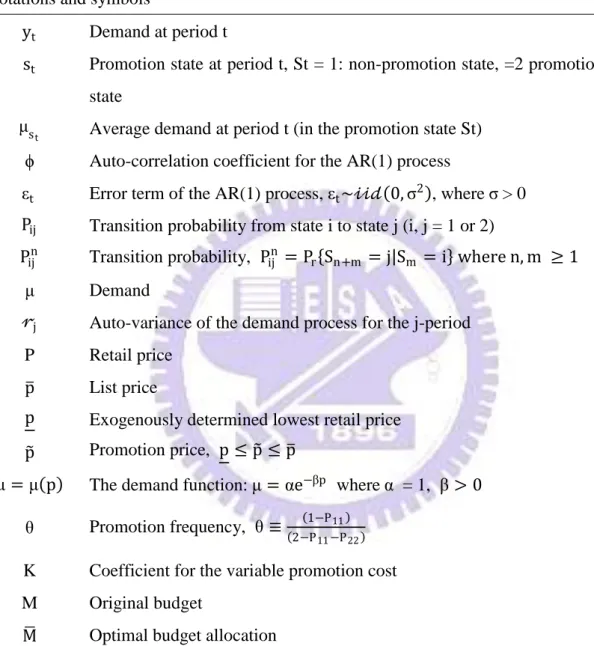
Where s_t represents the regime at time t, that is, s_t = 1 or 2, and ε_t~𝒾𝒾𝒹 0, σ2 . Note that all the symbols and notations are listed in Table 3-3. To apply a Markov switching time series model to promotion effects on demand, we make the following assumption:

Assumption 1:

For demand following the AR(1) process such as (1), assume that promotion activity increases by 𝛍, but that the correlation coefficient 𝛟 and error 𝛆𝐭 are unaffected.

In (1), the transition between regimes form one period to the next is considered a random variable that follows Markov chain properties. Thus, its transition probability is expressed as:

𝐏𝐫 𝐒𝐭 = 𝐣 𝐒𝐭−𝟏= 𝐢 = 𝐏𝐢𝐣 (2)

Here we name States 1 and 2 as the non-promotion state and the promotion state, respectively

In (1), ϕ is an auto-correlation coefficient. Lee et al. (2000) theoretically and empirically report that most commodities sold at retailers have positively-correlated demands. One interpretation of ϕ is brand loyalty. The stronger the brand loyalty, the higher the ϕ exhibited by the AR(1) process (Hanssens et al., 2001, p.253). The error term in the AR(1) model, ε_t , captures random shocks that the model cannot directly observe or control. For

21

instance, a change in the national economic environment can be understood as a random shock.

Table 3-3 Notations and Symbols Notations and symbols

yt Demand at period t

st Promotion state at period t, St = 1: non-promotion state, =2 promotion

state μ_s

t Average demand at period t (in the promotion state St)

ϕ Auto-correlation coefficient for the AR(1) process

εt Error term of the AR(1) process, εt~𝒾𝒾𝒹 0, σ2 , where σ > 0

Pij Transition probability from state i to state j (i, j = 1 or 2) P_ijn _{Transition probability, P}

ijn = Pr Sn+m = j Sm = i where n, m ≥ 1

μ Demand

𝓇j Auto-variance of the demand process for the j-period P Retail price

p List price

p Exogenously determined lowest retail price p Promotion price, p ≤ p ≤ p

μ= μ p The demand function: μ = αe−βp _{where α = 1, β > 0}

θ Promotion frequency, θ≡ 1−P11

2−P11−P22

K Coefficient for the variable promotion cost

M Original budget

M Optimal budget allocation

The period-expected profit becomes stable over several periods if stationary switching is assumed. Hence, we consider a Markov Switching time series model that has a stationary distribution. Set P_ijn = P_r S_n+m = j S_m = i where n, m≧1 for the N-state Markov chain. For the existence of a stationary distribution, which is defined as Pi = limn→∞Pijn > 0, the

22

ergodic Markov chain is covariance-stationary, and a time series process yt is defined as

covariance-stationary if neither the mean μ nor the auto-variance 𝓇_j of y_t depends on time. 𝐄 𝐲𝐭 = 𝛍 ∀𝐭 𝐚𝐧𝐝 𝐄 𝐲𝐭− 𝛍 𝐲𝐭−𝐣− 𝛍 = 𝓻𝐣 ∀𝐭 𝐚𝐧𝐝 𝐚𝐧𝐲 𝐣 (3)

Being covariance-stationary ensures the consistency of the model structure over time, which improves confidence in our analysis.

Remark1. In the case of the two-state Markov switching time series model, if the transition

probabilities satisfy 0 ≤ P₁₁, P₂₂ ≤ 1 and 0 ≤ P₁₁+ P₂₂ ≤ 1 , then the model is covariance-stationary; that is, the average profit is consistent over time and a stationary distribution exists.

Assumption 2:

(a) We consider only the stationary Markov switching process that satisfies Remark 1. (b) In addition to the stationary Markov switching process, we allow the case 𝐏_𝟏𝟏 =

𝟏 (𝐨𝐫 𝐏_𝟐𝟐 = 𝟏), where the demand process always belongs to State1 (or State 2).

3.4.4 Distribution of the two-state Markov switching AR(1) process

It is well-known that the variance of the AR(1) process y_t − μ_s

t = ϕ yt−1 − μst−1 + εt

where ε_t~𝒾𝒾𝒹. N 0, σ2 , is Var y_t = σ2/ 1 − ϕ2 . Here we set a stationary distribution probability of being in State 2 (i.e., the promotion state) as 0 ≤ θ ≤ 1, and, in a stationary Markov chain, θ is defined as

𝛉 = 𝛉 𝐏𝟏𝟏, 𝐏𝟐𝟐 = _𝟐−𝐏 𝟏−𝐏𝟏𝟏

𝟏𝟏−𝐏𝟐𝟐 (4)

A stationary distribution, θ, can be understood as the probability that manufacturer offers a promotion in a given period. Thus, we refer to θ as promotion frequency. θ in our model can be reasonably connected to a realistic promotion plan that actual manufacturers may apply. P₁₁ represents the manufacturers have a continuous non-promotion decision and P₂₂ represents they have a continuous promotion decision in two state. P12 represents they don‟t

23

in the period 1 but do not in the period 2. In the case of the two-state Markov switching time series model, if the transition probabilities satisfy θ ≤ P₁₁, P₂₂ ≤ 1 and 0 ≤ P₁₁+ P₂₂ ≤ 1, then the model is covariance-stationary.

Remark2.

(a) Period demand, yt, follows a normal distribution, such that

y_t~N θμ₁+ 1 − θ μ₂ , 1+ϕ 2 1 − ϕ2θ 1 − θ μ2− μ1 2 + σ2 1 − ϕ2

for the two-state Markov switching AR(1) time series process yt− μ_st = ϕ yt−1 − μ_st−1 +

ε_t where ε_t ~𝒾𝒾𝒹 N 0 , σ2 , and θ is the stationary probability of being in State 2. (b) E yt is decreasing and concave in P11, but increasing and convex in P22

(c) Var y_t is concave in θ, and maximized at θ = 0.5

3.4.5 Expected revenue for the manufacturer

We set the expected revenue, R, for the manufacturer as the product of the expected demand from customers, μ₁ or μ₂, and the discounted price p

𝐑 = 𝐑 𝐩 , 𝛉 = 𝟏 − 𝛉 𝐩 𝛍_𝟏+ 𝛉 𝐩 − 𝐤𝛉 𝛍_𝟐 𝐩 (5) Here we assume that the unit purchasing cost of the item is zero without loss of generality. Also the promotion cost is proportional to the promotion frequency, θ, and k is a coefficient of this linear promotion cost.

All the assumption and formula above (3.4.1~3.4.5) are from Hisashi and John‟s research in 2006 (European Journal of Operational Research 177, p1028~1032)

3.4.6 Optimal Sales Promotion plan

Based on Hisashi and John‟s research, we modify some part of them. We use the list price as a given exogenous variable, so the expected revenue, R, will as below:

24

𝐑 = 𝐑 𝛉 = 𝟏 − 𝛉 𝐩 𝛍𝟏+ 𝛉 𝐩 − 𝐤𝛉 𝛍𝟐 (6)

We take the first and second order derivatives of (6).

𝐅𝐎𝐂. 𝛛𝐑_𝛛𝛉 = −𝐩 𝛍𝟏+ 𝐩 − 𝟐𝐤𝛉 𝛍𝟐 , (7)

𝐒𝐎𝐂. 𝛛_𝛛𝛉𝟐𝐑_𝟐 = −𝟐𝐤𝛍𝟐 (8)

From Weierstrass theorem of the optimal value, the maximum point exist in the closed region of the decision variables, p, θ p = p , 0 ≤ θ ≤ 1 . Consequently, the maximum revenue is determined by the first order conditions (FOC):

−𝐩 𝛍_𝟏+ 𝐩 − 𝟐𝐤𝛉 𝛍_𝟐= 𝟎 (9) So the optimal promotion plan under maximized revenue condition is determined as follows (derived from (8)):

𝛉∗ ₌ 𝐩

𝟐𝐤𝛍𝟐 𝛍𝟐− 𝛍𝟏 (10)

If θ∗ is located below or above the boundaries, set θ∗= 1 or θ∗ = 0.  Optimal budget allocation

We could get θij crossing each type of promotion and every package.

∀ i = 1, 2, 3, 4

1 represents sum of all sales promotion, 2 represents coupon, 3 represents training expenditure, 4 represents display expenditure ∀ j = 1, 2, 3

1 represents Jar, 2 represents Cube, 4 represents bottle

Although θ_ij is to determine an optimal promotion frequency in a given period, it could also be a standard to allocate the budget. The bigger θ is, the more times promotion frequency is so that θ_ij is like a measurement of promotion performance while our sales promotion strategy is to maximize the profit.

25

We assume the total budget of these two categories, bouillons and seasonings, is M and the optimal budget allocation is M .

With M_i (except i=1, sum of all sales promotion, because when a=1 then M_a= M), we assign the budget of coupon, training expenditure, and display expenditure.

𝐌𝐢 = 𝐌 ×

𝛉𝐢𝐣 𝟑 𝐣=𝟏

𝛉𝐢 𝐣 𝐢𝐣 ; ∀ 𝐢 = 𝟐, 𝟑, 𝟒 (11)

According to θij, we could easily distribute the budget into each type of promotion across

every package.

𝐌𝐢𝐣 = 𝐌𝐢× 𝛉𝐢𝐣_𝛉

𝐢𝐣 𝟑

26

4. ANALYSIS

4.1 Linear Regression Model Analysis

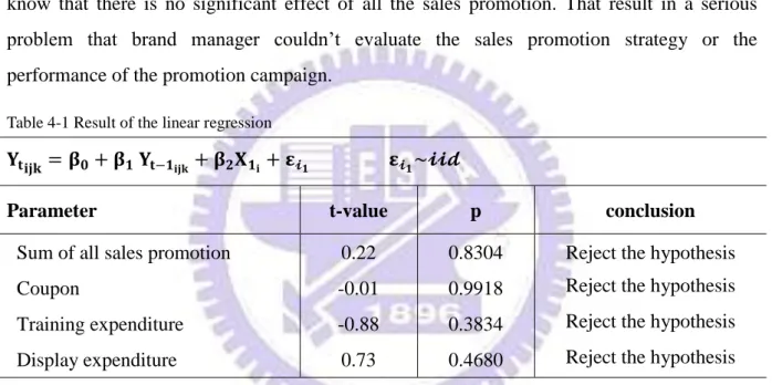
We examined the significance of the sales promotion acting on the sales performance. Here is the result of the examination in Table 4-1. P-value of a simple linear regression or a multiple linear regression is inside the blank. If p-value < 0.05, we could reject the null hypothesis that the parameter estimator of the independent variable is not equal to zero. We know that there is no significant effect of all the sales promotion. That result in a serious problem that brand manager couldn‟t evaluate the sales promotion strategy or the performance of the promotion campaign.

Table 4-1 Result of the linear regression

𝐘_{𝐭𝐢𝐣𝐤}= 𝛃𝟎+ 𝛃𝟏 𝐘𝐭−𝟏𝐢𝐣𝐤+ 𝛃𝟐𝐗𝟏𝐢+ 𝛆𝓲𝟏 𝛆𝓲𝟏~𝓲𝓲𝓭

Parameter t-value p conclusion

Sum of all sales promotion 0.22 0.8304 Reject the hypothesis

Coupon -0.01 0.9918 Reject the hypothesis

Training expenditure -0.88 0.3834 Reject the hypothesis

Display expenditure 0.73 0.4680 Reject the hypothesis

And then we examine the moderation effect. The testing result is shown in the Table

4-2.

Table 4-2 Result of the moderation effect

𝐘𝐭𝐢𝐣𝐤 = 𝛃𝟎+ 𝛃𝟏 𝐘𝐭−𝟏𝐢𝐣𝐤+ 𝛃𝟐 𝐗𝟏𝐢 + 𝛃𝟑 𝐗𝟐𝐣 + 𝛃𝟒 𝐗𝟏𝐢𝐗𝟐𝐣 + 𝛆𝓲𝟐 𝛆𝓲𝟐~𝓲𝓲𝓭

We set two dummy variables for three different packages.

Interaction F-value p conclusion

Sum of all sales promotion*packages 1.22 .2269 Reject the hypothesis .61 .5412 Reject the hypothesis

Coupon*packages .23 .8192 Reject the hypothesis

27

Training expenditure*packages .54 .5925 Reject the hypothesis

.87 .3843 Reject the hypothesis

Display expenditure*packages 1.43 .1565 Reject the hypothesis

.48 .6322 Reject the hypothesis 𝐘 = 𝛃_𝟎+ 𝛃_𝟏 𝐘_{𝐭−𝟏𝐢𝐣𝐤}+ 𝛃_𝟐 𝐗_𝟏𝐢+ 𝛃_𝟑 𝐗_𝟑𝐤+ 𝛃_𝟒 𝐗_𝟏𝐢𝐗_𝟑𝐤+ 𝛆_𝓲𝟑 𝛆_𝓲𝟑~𝓲𝓲𝓭

We set two dummy variables for three distinct outlets.

Interaction F-value p conclusion

Sum of all sales promotion*outlets 1.32 .1904 Reject the hypothesis -1.30 .1955 Reject the hypothesis

Coupon*outlets .24 .8138 Reject the hypothesis

-.83 .4089 Reject the hypothesis

Training expenditure*outlets -.45 .6562 Reject the hypothesis

-.03 .9750 Reject the hypothesis

Display expenditure*outlets 2.11 .0374* Significant

-1.00 .3205 Reject the hypothesis

Overall, the sales promotion strategy has no impact on stimulating sales and neither the moderation effect. The reason may be that it faced an acute competition with thousands of brands in the market or that it is in a market declined. Since the performance is not significant, how a brand manager weighs their budget on varied outlets, distinct categories, and different packages. Brand managers have to deal with two tough issues, how to allocate the budget among different categories, outlets, and packages and how the frequency of spending the money is, so that we introduce Markov Switching Model to solve the problems.

4.2 Markov Switching Model Analysis

We have several objectives introducing the Markov switching model. Table 4-3 summarizes θ with respect of sales promotion and different packages.

 Evaluating promotion performance

28

performance. θ ranged from 0 to 1. When θ = 0, it means past promotion investment hardly increasing the sales performance. First, coupon acted most on bottle package and so did training expenditure. Second, display expenditure plays an important role stimulating the sales of the cube. Overall sales promotion had greater impact on bouillons category (with sum of θ = .47) than seasoning category (with sum of θ =.34).  Budget allocation

Fist we could allocate total budget into different types of promotion.

𝐌_{𝐜𝐨𝐮𝐩𝐨𝐧} =. 𝟐𝟑𝐌 ; 𝐌_{𝐭𝐫𝐚𝐢𝐧𝐢𝐧𝐠𝐞𝐱𝐩𝐞𝐧𝐝𝐢𝐭𝐮𝐫𝐞} =. 𝟐𝟓𝐌 ; 𝐌_{𝐝𝐢𝐬𝐩𝐥𝐚𝐲𝐞𝐱𝐩𝐞𝐧𝐝𝐢𝐭𝐮𝐫𝐞}=. 𝟑𝟑𝐌 Based on the allocation of different types of promotion, 𝐌_𝐚 , we divided into each categories or packages. 𝐌_{𝐜𝐨𝐮𝐩𝐨𝐧−𝐉𝐚𝐫}=𝟏_𝟗𝐌 ; 𝐌_{𝐭𝐫𝐚𝐢𝐧𝐢𝐧𝐠𝐞𝐱𝐩𝐞𝐧𝐝𝐢𝐭𝐮𝐫𝐞−𝐉𝐚𝐫}= _𝟖𝟏𝟓 𝐌

𝐌_{𝐝𝐢𝐬𝐩𝐥𝐚𝐲𝐞𝐱𝐩𝐞𝐧𝐝𝐢𝐭𝐮𝐫𝐞−𝐂𝐮𝐛𝐞}=𝟑𝟑_𝟖𝟏𝐌 ; 𝐌_{𝐜𝐨𝐮𝐩𝐨𝐧−𝐁𝐨𝐭𝐭𝐥𝐞} =𝟏𝟒_𝟖𝟏𝐌 ; 𝐌_{𝐭𝐫𝐚𝐢𝐧𝐢𝐧𝐠𝐞𝐱𝐩𝐞𝐧𝐝𝐢𝐭𝐮𝐫𝐞−𝐁𝐨𝐭𝐭𝐥𝐞} =

𝟐𝟎 𝟖𝟐𝐌.

We have to notice that for some item, θ∗= 0, which means we assign no budget to the sales promotion on the packages. However, we emphasized providing a criterion to figure out the budget issues. We do not suggest that a brand manager use a random number generator to make a budget allocation decision.

Table 4-3 Summary of θ_ij

Bouillons Seasonings

Sum of θ

JAR CUBE BOTTLE

Coupon 0.09 ≈0 0.14 0.23

Training expenditure 0.05 ≈0 0.2 0.25

Display expenditure ≈0 0.33 ≈0 0.33

29  Optimal promotion frequency

According to Markov switching stationary distribution, we could calculate the possible transition probability combinations that can achieve from θ = θ P₁₁, P₂₂ =

1−P11

2−P11−P22 , which is constrained by θ ≤ P11, P22≤ 1 and 0 ≤ P11+ P22≤ 1, but that θ

is not uniquely decided by probabilities P₁₁ and P₂₂. So how a brand manager can apply the stochastic promotion result obtained by our model to real promotion planning?

For example, the model determines, say, θ21 = 0.09 for coupon on JAR package.

“P₁₁= 0.9 and P₂₂ = 0.0” could be a possible transition probability combinations that can achieve θ∗ = 0.09. In the two-state Markov chain, the average length that a manufacturer stays in the promotion state (or in the non-promotion state) is obtained as 1

1−P22 (or

1

1−P11). Thus P11= 0.9 and P22 = 0.0 can be interpreted as that a proper

length of staying non-promotion is ten months got non-promotion and one months for promotion in a year. So, in this case, the proposed promotion plan from our model will be offering a coupon an every ten month.

30

5. CONCLUSION

We analyzed the optimal sales promotion strategy, including budget allocation, promotion frequency and how to evaluate the promotion performance. Nowadays in a heavily competitive FMCG market, sales promotion could no longer guarantee stimulation of the sales and also too complicated to explain whether promotion works or not. So the manufacturer has trouble making the promotion decision. It is a dilemma that the effect of promotion seems to be uncertain but the promotion investment is getting larger proportion of the budget.

First we obtained a latest scanner data of a famous multinational packaged food company with rich information about sales, sales promotion, channels, and packages. Our result showed that indeed promotion didn‟t work out and so did the moderation effect. Second, We applied a Markov switching AR(1) process with the promotion and non-promotion regimes in order to capture the actual demand response to promotion. It is very important for a decision maker, brand manager or product manager, to make his promotion planning. Third, we not only try to figure out the actual demand response to promotion, but treat it as a criterion of budget allocation and further offer a promotion frequency decision. Base on θ∗ _we

could offer a standard to allocate our sales promotion budget on different packages or categories and we could also suggest a proper length of staying non-promotion state (or staying promotional state). Our study covers three steps of the category management, including planning merchandising, Implementing strategy and evaluating result.

Based on the Markov switching process and the optimal promotion frequency,θ∗_{, we}

generalize following rules for an optimal sales promotion strategy:

In such a competitive market, we should reduce the frequency of promotion. The Markov switching process has shown that θ∗ is quite low, which means the proposed promotion plan is offering at least every 8 months or longer. On the contrary, we should increase the investment on promotion plan each time. Because there are so many competitive products with their own promotion campaign in the market, consumer is in an information overloading condition. If the investment is not huge enough to deliver the

31

message against other promotion campaign to the consumer it would be less effective and waste a lot of money.

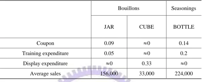
Table 5-1 Comparison table between average sales and θ

Bouillons Seasonings

JAR CUBE BOTTLE

Coupon 0.09 ≈0 0.14

Training expenditure 0.05 ≈0 0.2

Display expenditure ≈0 0.33 ≈0

Average sales 156,000 33,000 224,000

We could know from Table 5-1 that when the sales of a product were large, coupon and training expenditure had more impact on increasing sales. And while the sales of a product were small, display expenditure is a better choose of promotion plan. In our definition, display expenditure refers to the layout on the shelf, posters, event expenditure for display or road show, and shelf space which are ways to give a product more exposure to the consumer shopping in the store. Because there are too many similar products in this category, we need a specific way to get consumer‟s awareness especially for low-sales product. As to the coupon and training expenditure, when the sales of non-promotion state is large which imply higher awareness and more consumers so that promotion could easily accelerate their buying.

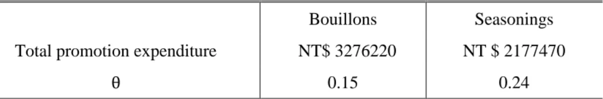
Our results also showed that higher promotion investment not necessarily comes out higher effectiveness. See Table 5-2. The reason for this consequence may be caused by consumer price sensitivity, brand awareness, substitutes, or consumer preference which is beyond the assumption in our study.

32

Table 5-2 Comparison table between promotion expenditure and θ

Bouillons Seasonings

Total promotion expenditure NT$ 3276220 NT $ 2177470

θ 0.15 0.24

However, we have some research limitation. First, we treat price as a given exogenous variable so that we did not consider the price discount effect in the retailer store and it would provide additional perspective. Second, we didn‟t consider the change in brand awareness, brand image and the impact on the customer‟s decision process. It provides some topics for the future study.

33

Reference

[1] Achabal, D.D., McIntyer, S., Smith, S.A. "Maximizing profits from periodic department score promotion", Journal of Retailing 66, (4), p383–407, 1990.

[2] Bemmaor, A. C. and D. Mouchoux, "Measuring the Short-Term Effect of In-Store Promotion and Retailer Advertising on Brand Sales" Journal of Marketing Research, 28 (May), p202-214, 1991.

[3] Blattberg C Robert, Richard Briesch, Edward J Fox "How Promotions Work" Marketing

Science, ABI/INFORM Global pg. G122, 1995.

[4] Bronnenberg, B.J. "Advertising frequency decisions in a discrete Markov process under a budget constrain", Journal of Marketing Research, 35 (3), p399–406. 1998.

[5] Chakravarthi Narasimhan, Scott A. Neslin, & Subrata K. Sen "Promotional Elasticities and Category Characteristics", Journal of Marketing, 60, ABI/INFORM Global pg. 17, Apr 1996.

[6] Chevalier, M. and R. C. Curhan, "Retail Promotion as a Function of Trade Promotions: A Descriptive Analysis", Sloan Management Review (Fall), 19-32, 1976.

[7] Curhan, R. C. and R. J. Kopp, "Factors Influencing Grocery Retailer‟s Support of Trade Promotions", Report No. 86-114, Cambridge, MA: Marketing Science Institute, July 1986.

[8] Friestad, Marian; Wright, Peter "The persuasion knowledge model: How people cope with persuasion attempts", Journal of Consumer Research, 1 p1-31, Jun 21, 1994.

[9] Ganesan, Shankar; Weitz, Barton A; John, "George Hiring and promotion policies in sales force management: Some antecedents and consequences", The Journal of Personal

Selling & Sales Management, 13, 2, ABI/INFORM Global pg. 15, Spring 1993.

[10] Hamilton J.D, "Analysis of Time Series Subject to Changes in Regime", Journal of

34

[11] Hamilton, J.D, Time Series Analysis. Princeton University Press, Princeton, NJ, 1994

[12] Hamilton, J.D "Specification testing in Markov-switching time-series models", Journal

of Econometrics, 70, p127–157, 1996

[13] Hissshi, K.&John,J.Liu "Optimal promotion planning-depth and frequency-for a two-stage supply chain under Markov switching demand", European Journal of

Operational Research, 177, p1026-1043, 2006.

[14] Jean-Marie Dufour, Maxwell L. King "Optimal invariant tests for the autocorrelation coefficient in linear regressions with stationary or nonstationary AR( 1) errors" Journal

of Econometrics, 47 115-143, 1991.

[15] Jeongwen Chiang "Competing Coupon Promotions and Category Sales", Marketing

Science, Vol14, No.1, Winter 1995.

[16] Kalwani, M.U., Yim, C.K. "Consumer price and promotion expectations: An experimental study" Journal of Marketing Research 29(1), 90–100., 1992.

[17] Kotler, P. & Keller, K.L., Principles of Marketing, Prentice Hall, 11th Edition, 2006.

[18] Kumar, V. and R. P. Leone, "Measuring the Effect of Retail Store Promotion on Brand and Store Substitution", Journal of Marketing Research, 25(May), 178-185, 1988.

[19] Leone P. Robert, Srinivasan S. Srini "Coupon face value: Its impact on coupon

redemptions, brand sales, and brand profitability", Journal of Retailing, Volume 72, Issue 3, Pages 273-289, Autumn 1996,

[20] Norm Borin, Paul W. Farris and James R. Freeland "A Model for Determining Retail Product Category Assortment and Shelf Space Allocation", Decision Sciences, 25, 3, ABI/INFORM Global, May/Jun 1994.

[21] Nielsen Marketing Research McGraw-Hill 1992

[22] Ronald W. Ward and James E. Davis "A Pooled Cross-Section Time Series Model of Coupon Promotions", American Journal of Agricultural Economics, Vol. 60, No. 3, pp. 393-401, Aug, 1978.

35

[23] Sanjay K. Dhar, Stephen J. Hoch, Nanda Kumar "Effective category management depends on the role of the category", Journal of Retailing, 77, p165–184, March 2001.

[24] Scott A. Neslin, Caroline Henderson and John Quelch "Consumer promotion and the acceleration of product purchases", Marketing Science, VoL4, No.2, Spring 1985.

[25] Sogomonian, A.G., Tang, C.S. "A modeling framework for coordinating promotion and production decisions within a firm", Management Science, 39 (2), p191–203, 1993.

[26] S. P. Meyn and R. L. Tweedie "Markov Chains and Stochastic Stability", London: Springer-Verlag, 1993.

[27] Suman Basuroy, Murali K. Mantrala, & Rockney G. Watlers "The impact of Category Management on Retailer Prices and Performance: Theory and Evidence", Journal of

Marketing, 65, 4, ABI/IMFORM Global pg.16, Oct 2001.

[28] Woodside, A. G. and G. L. Waddle, "Sales Effect of In-Store Advertising", Journal of