國立臺灣大學生命科學院生態學與演化生物學研究所 博士論文
Institute of Ecology and Evolutionary Biology, College of Life Science National Taiwan University
Doctoral dissertation
現行與未來氣候下的台灣森林植物分布預測研究 PREDICTING THE POTENTIAL DISTRIBUTIONS OF PLANT SPECIES AND FORESTS IN TAIWAN
UNDER PRESENT AND FUTURE CLIMATES 林奐宇
Huan-Yu Lin
指導教授:胡哲明教授 Advisor: Prof. Jer-Ming Hu
中華民國 109 年 3 月
March, 2020
誌謝
花了七個半年頭,終於寫出一部稍微完整的故事,從科學的角度講述臺灣森 林植群與氣候環境的關係。首要歸功於臺灣大學生態學與演化生物學研究所的兩 位老師—胡哲明教授與謝長富教授的多年指導、支持與科學訓練,使我的研究腳步 能夠踏得紮實穩固,在此致上無限感激。論文初成階段,得蒙王震哲教授、陳子英 教授、曾彥學教授及鍾國芳研究員指正,使文字表述臻於精準,更感謝諸位師長審 查過程中的觀點交換與討論激盪,讓本研究獲得許多未來的發展與想像。
這是一部由無數前人數據堆砌而成的論文。在展現研究成果之前,我必須慎 重地向諸多前輩表達我的敬意與謝意。包含曾經投入國家植群多樣性調查與製圖 計畫的師長、野外工作夥伴、調繪製圖與資料庫建置人員;林務局外來入侵植物調 查計畫團隊;臺灣四大植物標本館(TAI, TAIF, HAST, TNM)的標本採集與數位典 藏工作同仁;以及科技部臺灣氣候變遷推估資訊與調適知識平台(TCCIP)團隊。
由於眾多先進的支持,本論文才能站在充足的森林植物分布與氣候資料基礎上,對 臺灣森林植群與氣候的關係展開研究探索;也期許這篇論文能延續前輩的分享精 神,替臺灣未來的森林生態研究添磚加瓦,略盡一份棉薄之力。
猶記論文研究初期,單憑己力摸索著氣候變遷與物種分布的統計方法,頗有 摸石過河的無助與焦慮。感謝陳子英老師帶領我認識兩位貴人—不列顛哥倫比亞 大學(UBC)的王同立教授與王光玉教授,經由兩位師長的經驗技術傳授,以及亞 太森林復育與永續經營網絡(APFNet)的訓練課程支持,才使論文獲得長足進展。
此外,我的研究概念、邏輯思辨及統計方法,亦多得益於臺大森林系李靜峯教授、
關秉宗教授與邱祈榮教授。在此一併表達個人的點滴謝意。
這個博士學位,是在職進修獲得的。我的歷任服務單位,包含農林航空測量 所、林務局及林業試驗所,都為本研究提供了充足的調查資料、計畫經費與設備資
源。深切感謝臺灣林業部門的支持,也希望我的研究成果能回饋給林業界,對未來 的森林保育與經營管理做出貢獻。科學研究是一個快樂而充實的過程,然而,在工 作與進修並進下,難免壓縮了與家人共處的假日時光。謝謝我的家人,包括妻子、
父母及妹妹幫忙分擔了三個孩子的照顧工作,使我能專心處理研究工作疑難而免 於家庭牽掛,謹與我的所有親人,共享走完臺大學業段落的喜悅。
最後,借用指導教授胡哲明老師的一段講評:「這部論文除了整理出臺灣植物
分布的趨勢,更重要的,是它挖掘出更多值得探討的研究議題」。學術研究是沒有
止盡的,期望我的論文成果能作為後人探討森林生態的另一個起點,也期許來者秉 持合作分享的精神,擴大臺灣森林研究的力量。
於林業試驗所 2020 年 3 月
中文摘要
氣候與森林植物的分布緊密關連,而多項研究也證實,臺灣山地的帶狀植群分 化、以及部分泛域植群類型的分布,均與氣候條件高度相關,尤其受到溫度與年 間降水分配差異的影響。為瞭解臺灣森林植群與氣候的關係,進一步建立森林植 群氣候棲位資訊,以及推估氣候變遷的可能影響,本論文整合臺灣既有植群調查 及長期氣候資料,建立預測森林植物現生與未來分布的流程方法,並提出森林分 布變遷之研究結果。茲就各章節研究成果摘述如下:
一、動態氣候降尺度模型與高解析氣候圖層之產製
氣候資料是生態研究的重要基礎,然而一般泛用氣候圖資之空間解析度以數公里 至數十公里不等,難以反映山區起伏地形導致的氣溫與降水的劇烈變化。本章節 利用臺灣氣候變遷推估與資訊平台(TCCIP)5 公里網格氣候資料,經動態局部
迴歸方法獲得區域範圍之海拔遞減率,作為內插校正參數,於R 軟體設計一套自
由尺度化之氣候降尺度模型,命名為clim.regression。經 15 處不同海拔氣象測站
實測驗證,clim.regression 推估月尺度氣候之平均絕對誤差為 0.56°C(月均溫)、
0.79°C(月均低溫)、0.80°C(月均高溫)及 36.26mm(月累積降水),改善了 TCCIP 原始資料 54.6–66.7%的誤差。Clim.regression 共可針對歷史年度(1960–
2009)及三個未來階段產製 73 種氣候因子,其自由尺度化、高準確度的特色,
極適合在山地氣候與生態關係研究應用,亦是本論文進行後續章節研究之氣候資 料來源。
二、以氣候為基礎的臺灣山地植群分布模擬與預測方法
相較於傳統航遙測影像判釋或現場調查方法,森林植群氣候的棲位模擬預測,是 相對簡易而迅速獲得森林植群空間分布資訊的方法。本章節使用林務局國家植群 多樣性調查計畫樣區資料,以及李靜峯等人建立之森林分類架構,經由
clim.regression 產生各森林類型之氣候幅度,再利用隨機森林方法,建立 13 種與
氣候相關森林類型的棲位模型,並完成13 種森林類型的現生分布預測。依據
3817 個樣區交叉驗證顯示,隨機森林對於現生植群分布預測之平均錯誤率為 6.59%,森林分布預測結果與地形高度擬合,並反映出不同森林類型交會帶之過 渡現象。本章節證實高解析度、高準確度的氣候資料,配合野外調查樣本及充分 的機器學習訓練,可提供良好的植群現生分布資訊,作為預測未來變遷的基礎工 具。
三、海拔梯度下,氣候變遷對於臺灣山地森林植群的影響程度為何?
目前全球森林與氣候變遷相關研究,主要集中在北半球中緯度,對熱帶森林的研 究較少。以山地森林而言,普遍認為暖化可能導致森林植物的向上遷徙,對高海
拔或山頂植群造成威脅與衝擊。臺灣山地森林跨越近4000 公尺的海拔梯度,涵
蓋熱帶至亞高山森林類型,利用前一章獲得之山地植群模擬預測方法,於本章節 探討不同暖化情境下各森林類型的面積與海拔分布變化。所有暖化情境一致顯 示,高海拔森林及中海拔雲霧林可能出現面積縮減,尤其以亞高山刺柏灌叢及臺 灣水青岡落葉霧林首當其衝,將喪失大多數棲地(RCP 4.5)或瀕臨滅絕(RCP 8.5)。對於熱帶山地森林的預測結果則較為分歧,雖然熱帶森林的棲地面積在多 數暖化情境下呈現逐步擴張的趨勢,然而在極端暖濕、或極端暖乾的狀況下,可 能因水分有效性劇烈變化因素,導致熱帶山地霧林完全失去適存環境,熱帶季風 林亦將出現顯著的棲地縮減,是不可忽視的氣候變遷威脅。綜上研究結果,本章 節可推測出氣候變遷下的易危森林類型,並提出相對應的保育建議,作為後續監 測及管理工作的參考。
四、被子植物雌雄異株物種的地理分布與及其生態相關因子之研究
本論文收集大量的植物分布紀錄與氣候資料,不僅限於氣候變遷研究應用,也是 生態與生物地理分布研究的珍貴素材。本章節運用上述資料,以植物性別表現的 空間分布型式為例進行研究,希能激發其他生態研究者的興趣與更多的參與。
雌雄異株是相對罕見的植物生殖模式,藉由不同雌雄個體異交產生種子延續後
代。過去調查統計全球被子植物的雌雄異株種類約佔所有種類的6%,但許多例
子指出不同區域的雌雄異株物種比例會有差異,地形起伏劇烈的海洋島嶼、熱帶 森林、木本生活型、蟲媒授粉等現象,通常與較高的雌雄異株比例相關。臺灣的 地理環境具有大陸至海洋的過渡特性,本研究發現,臺灣本島被子植物的雌雄異
株整體比例約為8.2%,但從臺灣海峽至太平洋間,臺灣諸島被子植物相的雌雄異
株比例呈現逐漸升高的梯度,呼應了Bawa 氏提出的海洋島嶼較多雌雄異株物種
的理論。此外,沿本島海拔梯度則發現,自然植群皆存在雌雄異株比例隨海拔升
高而降低的現象,並在海拔2200 公尺處存在顯著的遞減率轉折點;高海拔的雌
雄異株比例劇烈陡降,推測可能與闊葉林與針葉林的交會轉換,以及高海拔授粉 昆蟲相趨於單純化所致。但人工植群之雌雄異株比例則與海拔無顯著相關。搭配 氣候因子分析,顯示雌雄異株植物常見於溫暖環境,兩性花植物則偏好於低溫的 高海拔地區,雜性物種的出現則與氣候條件無顯著關聯。
關鍵字:
氣候、氣候變遷衝擊、生態棲位模型、山地森林植群、隨機森林、臺灣
Abstract
Climate plays a vital role in shaping the distribution of forest and plant species. Some authors had reported that climate, especially the temperature and seasonal partitioning of rainfall, is significantly correlated with the altitudinal zonation of mountain forests and also to some of the distribution of azonal vegetation. This dissertation incorporated vegetation survey and historical climate data to reconstruct climatic niches for mountain forests of Taiwan, and project their distributional changes under future climatic scenarios.
The critical outcomes of each chapter summarized as below:
1. A dynamic downscaling approach to generate scale-free regional climate data.
Climate variables, particularly temperature and precipitation, are the most well- known key factors related to vegetation zonation. However, to obtain climate data adequately for the requirement of ecological studies is challenging due to the difficulty of data integration and the complexity of downscaling, especially for mountainous regions. In this section, a synthetic approach combining bilinear interpolation and dynamic local regression was conducted to develop a scale-free climate downscaling model in R environment, namely clim.regression. Based on the original 5km x 5km gridded climate surface from TCCIP, clim.regression can generate 73 climatic variable estimates specific to the user-defined points of interest for historical (1960–2009) and future periods (2016–2035, 2046–2065 and 2081–2100), which reduced prediction error by 54.6–66.7% relative to the original gridded climate data for temperatures. The result is adapted to the uses of ecological researches and is the source of climate data of this dissertation.
2. Climate-based approach for modeling the distribution of montane forest
A climate-based ecological niche model may provide an effective alternative to the traditional approach for assessing limitations, thresholds, and the potential distribution of forests. In this section, a machine-learning method based on scale-free climate variable estimates and classified vegetation plots was applied to develop niche models for the 13 climate-related forest types in Taiwan, and to generate a fine-scale predicted vegetation map. The result supported that the machine-learning approach is sufficient to handle a large number of variables and to provide accurate predictions, which has the potentials in projecting the distributional changes of forests under different climate change scenarios.
3. How much does climate change alter the distribution of forests across a great altitudinal gradient?
Taiwan is a high-mountain island with substantial altitudinal variations and diverse forest types driven by climate. In this study, we used the scale-free climate variable estimates and an established machine-learning approach to project the distributional changes of 13 climate-related mountain forest types under selected global warming scenarios. The results demonstrated a consistent trend of the drastic habitat contractions of subalpine Juniperus woodland and the deciduous Fagus broadleaved forests. It also revealed that tropical montane cloud forest and tropical winter monsoon forest might be highly vulnerable under the extreme warm-humid or warm- dry climatic conditions because of the sever change of water availability. For mitigating the risk of climate change to the vulnerable forest types, adapted conservation strategies were suggested according to the environmental characteristic of each forest type.
4. Geographical distribution of dioecy and its ecological correlates based on fine-
scaled species distribution data.
A great deal of species occurrence and climate data is valuable in different ecological researches. An example is shown here to demonstrate such use in elucidating the complicate distribution patterns of plant sexual systems. In this section, I used species occurrence and historical climate data in exploring the geographical distribution of sexual expression systems of the flowering plants in Taiwan.
It was reported that the incidence of dioecy varied among local floras and suggested inclining to tropical and oceanic environments. We found the average incidence of dioecy in the flora of Taiwan to be 8.2%, but it exhibits geographical variations from islets in the Taiwan Strait to the Pacific Ocean. An apparent two-step decreasing pattern of dioecy percentages with elevation was also found, which shows a distinct transition at the altitude of 2200m. The overall analysis indicated that spatial variations of dioecy were associated with eco-correlates of land cover, elevation, woodiness, species richness, and mean annual temperature. Results of this section partially support Bawa’s hypothesis of a higher incidence of dioecy on oceanic islands, and consistent with Baker and Cox’s observations of more prosperous dioecious species on high-mountain islands in the tropics and subtropics.
Key words:
Climate, Climate change impacts, Ecological niche modeling, Mountain forest vegetation, Random forest, Taiwan.
Comparison table of abbreviations
Abbreviation Definition
AR5 The IPCC Fifth Assessment Report. AR5 is a report announced by IPCC in 2014, it provides an overview of the state of knowledge concerning the science of climate change, emphasizing new results since the publication of the IPCC Fourth Assessment Report (AR4) in 2007.
(https://www.ipcc.ch/report/ar5/syr/)
CMIP5 The Coupled Model Intercomparison Project (CMIP) is a standard experimental framework for studying the output of coupled atmosphere-ocean general circulation models. CMIP5 is the most current and extensive of the CMIPs. The objectives of CMIP5 are to:
1. evaluate how realistic the models are in simulating the recent past,
2. provide projections of future climate change on two time scales, near term (out to about 2035) and long term (out to 2100 and beyond), and
3. understand some of the factors responsible for differences in model projections, including quantifying some key feedbacks such as those involving clouds and the carbon cycle.
(https://climatedataguide.ucar.edu/climate-model-evaluation/cmip- climate-model-intercomparison-project-overview)
CoDeK Cocktail determination key. CoDeK is a software application, based
Abbreviation Definition
on R program (R Development Core Team 2012), which allows automatic classification of vegetation samples into vegetation types defined by Cocktail determination key. The Cocktail Determination Key has been published as supplementary materials in Li et al.
(2013), it allows automatic assignment of vegetation plots into predefined vegetation types (supervised classification).
(https://www.davidzeleny.net/doku.php/software)
GCM General circulation model. GCM is a type of climate model. It employs a mathematical model of the general circulation of a planetary atmosphere or ocean based on the basic laws of physics, fluid motion, and chemistry. Scientists divide the planet into a 3- dimensional grid, apply the basic equations, and evaluate the results.
The calculations include winds, heat transfer, radiation, relative humidity, and surface hydrology within each grid and evaluate interactions with neighboring points.
(https://en.wikipedia.org/wiki/General_circulation_model)
IPCC Intergovernmental Panel on Climate Change. IPCC is the United Nations body for assessing the science related to climate change. It provides regular assessments of the scientific basis of climate change, its impacts and future risks, and options for adaptation and mitigation.
(https://www.ipcc.ch/)
LGM Last Glacial Maximum. LGM was the most recent time during the
Abbreviation Definition
Last Glacial Period that ice sheets were at their greatest extent. The growth of ice sheets commenced 33,000 years ago and maximum coverage was between 26,500 years and 19–20,000 years ago.
(https://en.wikipedia.org/wiki/Last_Glacial_Maximum)
LOESS Local polynomial regression. LOESS is a nonparametric technique for smoothing scatter plots and modeling functions. For each point, x0, a low-order polynomial regression is fit using only points in some
“neighborhood” of x0. The result is a smooth function over the support of the data.
Avery, M. (2010). Literature Review for Local Polynomial Regression.
MAP Mean annual precipitation. It refers to the sum of precipitation of 12 months a year.
MAT Mean annual temperature. It refers to the average of mean temperatures of 12 months a year.
OOB error Out-of-bag error. OOB error is a method of measuring the prediction error of random forests, boosted decision trees, and other machine learning models utilizing bootstrap aggregating (bagging) to sub-sample data samples used for training. Subsampling allows one to define an out-of-bag estimate of the prediction performance improvement by evaluating predictions on those observations which were not used in the building of the next base learner.
Abbreviation Definition
(https://en.wikipedia.org/wiki/Out-of-bag_error)
RCP Representative Concentration Pathways. RCPs usually refer to the portion of the concentration pathway extending up to 2100, corresponding emission scenarios. Four RCPs, RCP 2.6, RCP 4.5, RCP 6.0, and RCP 8.5, produced from Integrated Assessment Models were selected from the published literature and are used in the Fifth IPCC Assessment as a basis for the climate predictions and projections.
(https://www.ipcc-
data.org/guidelines/pages/glossary/glossary_r.html)
RF Random forests. RF is an ensemble learning method for classification, regression and other tasks that operate by constructing a multitude of decision trees at training time and outputting the class that is the mode of the classes (classification) or mean prediction (regression) of the individual trees. This method has been recommended for modeling the ecological niche of organisms and predicting their potential distribution.
(https://en.wikipedia.org/wiki/Random_forest)
TCCIP Taiwan Climate Change Information and Projection. The TCCIP coordinated by National Science and Technology Center for Disaster Reduction (NCDR) is one of the major climate change projects funded by Ministry of Science and Technology. The TCCIP project
Abbreviation Definition
not only produces climate change data for impact assessments and adaptations but also aims to support national adaptation policy framework.
(https://tccip.ncdr.nat.gov.tw/au_eng.aspx)
Contents
口試委員會審定書 i
誌謝 iii
中文摘要 v
Abstract viii
Comparison table of abbreviations xi
Chapter 1. General introduction 1-1
Chapter 2. A dynamic downscaling approach to generate scale-free regional climate data in Taiwan
2.1 Introduction 2-2
2.2 Materials and methods 2-4
2.3 Results 2-11
2.4 Discussion 2-25
2.5 Author contributions 2-30
2.6 Literature cited 2-30
Chapter 3. Climate-based approach for modeling the distribution of montane forest vegetation in Taiwan
3.1 Introduction 3-2
3.2 Materials and methods 3-6
3.3 Results 3-13
3.4 Discussion 3-24
3.5 Author contributions 3-31
3.6 Literature cited 3-32
Chapter 4. How much does climate change alter the distribution of forests across a great altitudinal gradient on a subtropical island?
4.1 Introduction 4-2
4.2 Materials and methods 4-6
4.3 Results 4-11
4.4 Discussion 4-24
4.5 Author contributions 4-29
4.6 Literature cited 4-29
Chapter 5. Geographical distribution of dioecy and its ecological correlates based on fine-scaled species distribution data from a subtropical island
5.1 Introduction 5-2
5.2 Materials and methods 5-5
5.3 Results 5-10
5.4 Discussion 5-20
5.5 Author contributions 5-25
5.6 Literature cited 5-25
Supplementary: Committee’s comments and the responses S-1
Chapter 1 General introduction
Climate is one of the most important factors shaping the distribution of species, communities, ecosystems, and biomes (Whittaker, 1975; Woodward and Williams, 1987;
Davis and Shaw, 2001). To understand the vegetation-climate relationship is not only the kernel that most ecologists interested in but also being a piece of equipment for exploring the possible changes of organisms in a changing environment. Anthropogenic climate change in recent decades has emerged as a major driver affected the characteristics of vegetation worldwide, such as the directional range shift of plants and animals (IPCC, 2014), the disrupted interspecies phenological synchrony (Ovaskainen et al., 2013), and local extinction events in particular localities (Pauli et al., 2012), which may cause severe impacts to the management of natural resources, biological conservation, and ecosystem functions and services.
The directional range shift, including the poleward and upward migration of species under global warming, is an issue of growing concern for many ecologists. A first-order approximation regarding the response of organisms to a warming climate is that species will migrate upward or poleward to find a suitable climate to survive (Beniston, 2003).
Mountain environment is a region with dramatic climatic gradient in a very short distance that species could find and access a cooler habitat easily. However, the accompanied competition, substitution, and progressively replacement of mountain forest communities may also occur.
Taiwan is a mountainous island with territories over 70% occupied by hills and mountains, and a total of 58% of this island is covered by forests. It’s already known that regional climate, especially the altitudinal temperature gradient and seasonal precipitation
differences, shapes the diverse mountain forests of Taiwan (Su, 1984). Since mountain forest vegetation plays important role in harboring the plentiful biodiversity of our home island, it is needed to study the relationship of forest vegetation with the concurrent climatic environment, and to map the possible influence of climate change on forest ecosystems. The results, e.g. the estimated range shift of a specific or a rare forest type in the coming decades, can be applied in the use of protected area evaluation or threatened species conservation.
Studies of niche modeling for plant species/communities were launched around 20 years in Taiwan (Lee et al., 2006), and the climatic characteristics of a few species (Yen et al., 2008; Nakao, et al., 2014; Lin and Chiu, 2019) or forest types (Chiu et al., 2013; Lin et al., 2014) have been reported accordingly. However, intact modeling for the distribution of forests at the whole-island scale and the assessment for their future change have still received little research attention. Furthermore, most climatic niche modeling studies used the worldwide and online accessible climate database such as WorldClim (Hijmans, et al., 2005), rather than using the fine-scale interpolated climatic surface from historical observations of local meteorological stations. Weng and Yang (2012) compared the prediction accuracy between East-Asia regional climate model and Taiwan’s local observations, and they utilized historical data from thousands of local meteorological stations to establish a gridded climate surface improving the performance of regional climate model. From 2012 on, a gridded climate surface covers the historical period of 1960–2012 and the future stages of 2016–2035, 2046–2065, and 2081–2100 was released by Taiwan Climate Change Projection and Information Platform (TCCIP), which has become the ideal and fundamental materials for conducting climate-relevant researches.
In this dissertation, my research goal is to incorporate the plant distribution data and the
latest released climate surface to model the concurrent vegetation-climate relationship at the whole-island scale, which can be applied in projecting the change of forest distribution under different climate change scenarios. The main layouts of this study were stated as follows:
(1) Accurate and fine-resolution climate data is essential for modeling forest distribution corresponding to the diverse topography in the mountains. We developed a statistical approach to downscale the 5 km x 5 km climate data provided by TCCIP to a scale- free format being environmental factor estimates for the climate niche models.
(Chapter 2)
(2) Establishment of a climate-based approach for modeling the vegetation-climate relationship based on field sampling data and its corresponding climatic parameters.
This model framework can be used to generate a predicted vegetation map under the selected climatic scenario. (Chapter 3)
(3) An extended application of the vegetation-climate model. Based on climate data of different general circulation models (GCMs) and emission scenarios provided by TCCIP, we explored the possible change of forest distribution, including the area change and altitudinal range shift, and to evaluate the impact of climate change on each forest type. (Chapter 4)
(4) A further example of using the developed data from above. I used the geographical distribution of plant sexual expression system in Taiwan as an example to illustrate the extended application of our data. It would be an ideal demonstration for more ecological studies to be involved in. (Chapter 5)
LITERATURE CITED
Beniston, M. 2003. Climatic change in mountain regions: A review of possible impacts.
Climatic Change 59: 5–31.
Chiu, C.-A., T.-Y. Chen, C.-C. Wang, C.-R. Chiou, Y.-J. Lai and C.-Y. Tsai. 2013.
Using BIOMOD2 to model the species distribution of Fagus hayatae. Quarterly Journal of Forest Research 35: 253–272. [In Chinese with English summary.]
Davis, M. B. and R. G. Shaw. 2001. Range shifts and adaptive responses to quaternary climate change. Science 292: 673–679.
Hijmans, R. J., S. E. Cameron, J. L. Parra, P. G. Jones and A. Jarvis. 2005. Very high resolution interpolated climate surface for global land areas. International Journal of Climatology 25(15): 1965–1978. http://doi.org/10.1002/joc.1276 IPCC. 2014. Summary for policymakers. In: Climate Change 2014: Impacts,
adaptation, and vulnerability. Part A: Global and sectoral aspects. Contribution of Working Group II to the Fifth Assessment Report of the Intergovernmental Panel on Climate Change. Cambridge University Press, Cambridge, United Kingdom and New York, NY, USA, pp. 1–32.
Lee, P.-F., K.-Y. Lue and S.-H. Wu. 2006. Predictive distribution of Hynobiid salamanders in Taiwan. Zoological Studies 45: 244–254.
Lin, C.-T. and C.-A. Chiu. 2019. The relic Trochodendron aralioides Siebold & Zucc.
(Trochodendraceae) in Taiwan: Ensemble distribution modeling and climate change impacts. Forests 10(1): 7. http://doi.org/10.3390/f10010007
Lin, W.-C., Y.-P. Lin, W.-Y. Lien, Y.-C. Wang, C.-T. Lin, C.-R. Chiou, J. Anthony and N. D. Crossman. 2014. Expansion of protected areas under climate change: An example of mountainous tree species in Taiwan. Forests 2014(5): 2882–2904.
Nakao, K., M. Higa, I. Tsuyama, C.-T. Lin, S.-T. Sun, J.-R. Lin, C.-R. Chiou, T.-Y.
Chen, T. Matsui and N. Tanaka. 2014. Changes in the potential habitats of 10 dominant evergreen broad-leaved tree species in the Taiwan-Japan archipelago.
Plant Ecology 215: 639–650.
Ovaskainen, O., S. Skorokhodova, M. Yakovleva, A. Sukhov, A. Kutenkov, N.
Kutenkova, A. Shcherbakov, E. Meyke and M. M. Delgado. 2013. Community- level phenological response to climate change. PNAS 110(33): 13434–13439.
Su, H.-J. 1984. Studies on the climate and vegetation types of the natural forests in Taiwan (II). Altitudinal vegetation zones in relation to temperature gradient.
Quarterly Jounal of Chinese Forestry 17(4): 57–73.
Whittaker, R. H. 1975. Communities and ecosystems. 2nd Revise Edition, MacMillan Publishing Co., New York.
Weng, S.-P. and C.-T. Yang. 2012. The construction of monthly rainfall and
temperature dataset with 1km gridded resolution over Taiwan area (1960–2009) and its application to climate projection in the near future (2015–2039). Atmospheric Sciences 40(4): 349–369. [in Chinese with English summary]
Woodward, F. I. and B. G. Williams. 1987. Climate and plant-distribution at global and local scales. Vegetatio 69: 189–197.
Yen, S.-M., C.-R. Chiou and K.-T. Chang. 2008. Modeling the species distribution of three dominant coniferous species in Taiwan. Taiwan Journal of Forest Science 23(2): 165–181.
Chapter 2
A dynamic downscaling approach to generate scale-free regional climate data in Taiwan
This chapter is a published paper in Taiwania 63(3): 251–266, 2018, co-authored by Huan-Yu Lin, Jer-Ming Hu, Tze-Ying Chen, Chang-Fu Hsieh, Guangyu Wang, and Tongli Wang.
Abstract
Plenty of climate data from various sources have become available in recent years.
However, to obtain climate data adequately meeting the requirement of ecological studies remains a challenge in some cases due to the difficulty of data integration and the complexity of downscaling, especially for mountainous regions. Lapse rate is one of the most important factors that influence the change of climatic variables in the mountains, and it should be incorporated into climatic models. In this study, we applied a synthetic approach combining bilinear interpolation (to produce seamless surfaces) and dynamic local regression (to obtain local lapse rates) to develop a scale- free and topography-correspondent downscaling model in R environment for Taiwan, called clim.regression. This model can generate 73 climatic variable estimates specific to the user-defined points of interest, including primary climatic variables and additional biologically relevant derivatives for historical (1960–2009) and future periods (2016–2035, 2046–2065 and 2081–2100). Results of our evaluation indicated that clim.regression reduced prediction error by 54.6%–66.7% relative to the original gridded climate data for temperatures. In addition, we demonstrated the spatiotemporal patterns of lapse rate for different climate variables.
KEY WORDS: Climate change, Downscaling model, Dynamic local regression, Historical and future climate scenarios, TCCIP.
INTRODUCTION
Climate variables, particularly temperature and precipitation, are the most well-known key factors related to vegetation zonation. A high-quality and accessible climate dataset is essential for ecological studies and applications, especially in regions with diverse topography and high climatic heterogeneity. However, to obtain and to process substantial climate data were difficult for ecologists in the past, and scientists often use statistically interpolated climate data from a few existing stations as substitutes for the continuous climate surface (Su, 1984a; Tang and Ohsawa, 1997).
Over the last decade, a large volume of climate data has become available through various sources; most of them were represented in grid format with the finest resolution of arc- seconds or kilometers in global or regional scale (Hannaway et al., 2005; Hijmans et al., 2005; Harris et al., 2014). Although such gridded data are suitable for modeling general patterns and trends at global and regional scales, they are still too coarse to provide detailed climatic information in mountainous and topographically diverse areas to facilitate local ecological studies and resources management. To overcome this limitation, several downscaling methods have been developed to generate high-resolution spatial climate data, such as Ordinary Kriging (Chiu and Lin, 2004), a combination of Kriging and polynomial linear regression (Chiou et al., 2004), a combination of bilinear interpolation and partial derivative functions for elevational adjustment (Wang et al., 2006;
2012), and an approach of dynamic local regression (Wang et al., 2016; 2017). ClimateAP,
recently developed and covered Asia-Pacific (AP) region (Wang et al., 2017). The baseline data of this model used a 4-km gridded climate data from PRISM (Daly et al., 2002) for China and Mongolia, and WorldClim (Hijmans et al., 2005) for the rest of the Asia-Pacific. The model reduces prediction error by up to 27% and 60% for monthly temperature and precipitation, respectively, relative to the original baseline data. However, the prediction accuracy for a specific region varies depending on the quality of the baseline data, which is affected by the density of weather stations used for developing the baseline data for the region. Unfortunately, historical climate data from weather stations in Taiwan were not included in the climate mapping project of PRISM (Hannaway et al., 2005). Thus, it could adversely impact the prediction accuracy of ClimateAP in Taiwan.
Taiwan is a subtropical island on the west edge of the Pacific Ocean with diverse and complicated topography. The climate of Taiwan is mainly affected by the northeast monsoon during winter and by the southwest monsoon and typhoons in the summer. The Central Range occupying more than 70% of the area of Taiwan, runs through the whole island from northeast to southwest with the highest peak of 3,952 meters asl, and creates an obvious altitudinal temperature zonation (Su, 1984a), as well as the seasonal allocation of precipitation (Su, 1985). Many studies have revealed a strong relationship between the natural vegetation and the large-scale altitudinal climate zonation (Su, 1984b; Chiu, 2004;
Chiou et al., 2010; Lin et al., 2012; Li et al., 2013). Furthermore, the local climate is induced by the co-effects of monsoon and topography (Sun, 1993; Sun et al., 1998; Chao et al., 2007; Chao et al., 2010; Li et al., 2013). Ecologists have a strong demand on fine- scale climate data to depict the ecological and environmental correlations in detail.
However, most studies can only utilize indirect variables such as elevation and topography as substitutes to climatic variables due to the lack of a high-quality and high- resolution spatial climate dataset for the island.
Meteorologists in Taiwan have accomplished a framework called Taiwan Climate Change Projection and Information Platform (TCCIP) and generated a 5km × 5km gridded climate surface based on historical observations from thousands of weather stations and provided future projections based on different AR5 General Circulation Models (GCMs) and scenarios (Hsu et al., 2011; Weng and Yang, 2012). TCCIP’s datasets are powerful supplements to the remote and observation-sparse mountains, but its resolution is not fine enough to represent the diverse climate situation due to the steep topography within a 5km × 5km grid.
In this study, our main objectives were to: (1) establish a statistical downscaling model named as clim.regression in R environment to downscale the 5km × 5km gridded climate data of TCCIP to a scale-free format based on the algorithm of bilinear interpolation and dynamic local regression from ClimateNA (Wang et al., 2016) and ClimateAP (Wang et al., 2017); (2) generate additional biologically relevant derivatives for ecological studies;
(3) analyze the spatiotemporal patterns of variation in lapse rate; and (4) evaluate the prediction accuracy of clim.regression in comparison to the original TCCIP data.
MATERIALS AND METHODS
Source of historical and future climate data
The 5km × 5km gridded surfaces of historical meteorological data used in this study were developed by TCCIP (Weng and Yang, 2012). The dataset covers the main island of Taiwan and spans the period from 1960 to 2009. TCCIP incorporated historical records of air temperature from 1,152 weather stations and precipitation from 1,497 rainfall stations to construct the gridded dataset through a conventional spatial interpolation process. There are four sets of primary climate variables including monthly precipitation
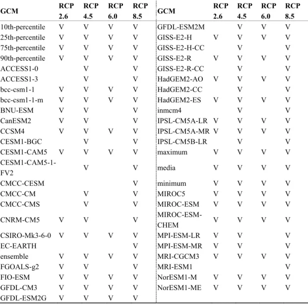
mean temperature (Tmean01 to Tmean12) and monthly maximum temperature (Tmax01 to Tmax12). The values of these variables were obtained and united with the coordinate (latitude, longitude and elevation) of the center of each grid. There were 48 primary monthly climate variables in total. TCCIP has also provided future climate projections in the same resolution of 5km × 5km, which were downscaled from GCMs of CMIP5 and rectified by observations of Aphrodite (Asia Precipitation Highly-Resolved Observational Data Integration Towards Evaluation of the Water Resources) and historical climate data of Taiwan (Lin et al., 2016). Projections of 49 GCMs (Table 2.1) covering different RCPs (RCP 2.5, RCP 4.6, RCP 6.0 and RCP 8.5) and periods (2016–
2035, 2046–2065, 2081–2100).
The downscaling process of historical and future climate data
To obtain smooth and continuous climate surface estimates, clim.regression utilized the combination of bilinear interpolation and dynamic local regression approach to downscale the original 5km × 5km gridded climate dataset to scale-free point estimates, which is the same as in ClimateNA (Wang et al., 2016) and ClimateAP (Wang et al., 2017).
The downscaling process included four steps for each of the 48 primary monthly climate variables as illustrated in Fig. 2.1:
(1). Extraction of a primary climate variable and elevation from the grid covering the point of interest and eight neighboring grids (Fig. 2.1A);
(2). Calculation of the bilinear interpolated estimate of the primary monthly climate variable (t’p) and elevation (Z’p) of the location of interest from the nearest four grids (Fig. 2.1B, Formula 1 & 2);
(3). Calculation of the differences in the primary monthly climate variable (∆t) and in
elevation (∆z) between each of the 36 unique pairs among the nine neighbor grids (Fig. 2.1C, Formula 3);
(4). Construction of a simple linear regression based on the 36 pairs to represent the local relationship between ∆t and ∆z with the slope of the regression line, m, representing the local lapse rate of the cell where the interest point is located. Elevation adjustment was based on the lapse rate (m) and the difference between actual elevation (Zp) and the bilinear interpolate (Z’p) of the interest point (Fig. 2.1D, Formula 4).
Table 2.1. All the 49 GCMs and emission scenarios provided by TCCIP available for clim.regression.
GCM RCP
2.6
RCP 4.5
RCP 6.0
RCP
8.5 GCM RCP
2.6
RCP 4.5
RCP 6.0
RCP 8.5
10th-percentile V V V V GFDL-ESM2M V V V
25th-percentile V V V V GISS-E2-H V V V V
75th-percentile V V V V GISS-E2-H-CC V V
90th-percentile V V V V GISS-E2-R V V V V
ACCESS1-0 V V GISS-E2-R-CC V V
ACCESS1-3 V V HadGEM2-AO V V V V
bcc-csm1-1 V V V V HadGEM2-CC V V
bcc-csm1-1-m V V V V HadGEM2-ES V V V V
BNU-ESM V V V inmcm4 V V
CanESM2 V V V IPSL-CM5A-LR V V V V
CCSM4 V V V V IPSL-CM5A-MR V V V V
CESM1-BGC V V IPSL-CM5B-LR V V
CESM1-CAM5 V V V V maximum V V V V
CESM1-CAM5-1-
FV2 V V media V V V V
CMCC-CESM V minimum V V V V
CMCC-CM V V MIROC5 V V V V
CMCC-CMS V V MIROC-ESM V V V V
CNRM-CM5 V V V MIROC-ESM-
CHEM V V V V
CSIRO-Mk3-6-0 V V V V MPI-ESM-LR V V V
EC-EARTH V MPI-ESM-MR V V V
ensemble V V V V MRI-CGCM3 V V V V
FGOALS-g2 V V V MRI-ESM1 V
FIO-ESM V V V V NorESM1-M V V V V
GFDL-CM3 V V V V NorESM1-ME V V V V
GFDL-ESM2G V V V V
Fig. 2.1. Four steps of the downscaling process. (A) The grid tiles covering the point of interest p and its eight neighbors were extracted from the original climate dataset. (B) Bilinear interpolated estimates of temperature, precipitation and elevation of the point p were calculated by the weighting of distance to the center of the four nearest grid tiles. (C) A total of 36 unique pairs were subset to calculate the paired differences for temperature, precipitation (∆t) and elevation (∆z), respectively. (D) A simple linear regression of Δtmn~ΔZmn was conducted to obtain the slope m, representing the local lapse rate of the nine grids surround point of interest for each of the climate variables.
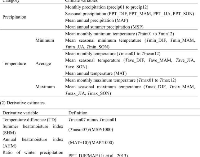
Clim.regression generated 73 climate variable estimates (Table 2.2) for either a single point location or a continuous surface. These climate variables were either directly calculated from the four primary climate variables or derived as indicated in Table 2.2.
The formula for the downscaling process included:
𝑡𝑝′=𝑡1𝑑2𝑑4+ 𝑡2𝑑2𝑑3+ 𝑡3𝑑1𝑑3+ 𝑡4𝑑1𝑑4 𝑑2
(1)
(2)
(3)
(4)
𝑍𝑝′=𝑍1𝑑2𝑑4+ 𝑍2𝑑2𝑑3+ 𝑍3𝑑1𝑑3+ 𝑍4𝑑1𝑑4 𝑑2
∆𝑡𝑚𝑛~Δ𝑍𝑚𝑛, 𝑚 = 1,2,3, … ,9 , 𝑛 = 1,2,3, … ,9 , 𝑚 ≠ 𝑛 𝑡𝑝 = 𝑡𝑝′ + 𝑚 𝑍𝑝− 𝑍𝑝′
Future climate projections of TCCIP were presented as anomalies relative to the baseline of 1986–2005 at the same spatial resolution of historical climate data. The anomalies of 5km × 5km gridded future climate projections were added to the baseline portion (1986–
2005) to create a ‘gridded future climate data’ prior to the downscaling procedure.
Table 2.2. Primary climate variables and the biologically relevant derivatives generated by clim.regression
(1) Primary climate variable estimates.
Category Climate variables
Precipitation
Monthly precipitation (precip01 to precip12)
Seasonal precipitation (PPT_DJF, PPT_MAM, PPT_JJA, PPT_SON) Mean annual precipitation (MAP)
Mean annual summer precipitation (MSP)
Temperature
Minimum
Mean monthly minimum temperature (Tmin01 to Tmin12)
Mean seasonal minimum temperature (Tmin_DJF, Tmin_MAM, Tmin_JJA, Tmin_SON)
Average
Mean monthly temperature (Tmean01 to Tmean12)
Mean seasonal temperature (Tave_DJF, Tave_MAM, Tave_JJA, Tave_SON)
Mean annual temperature (MAT)
Maximum
Mean monthly maximum temperature (Tmax01 to Tmax12)
Mean seasonal maximum temperature (Tmax_DJF, Tmax_MAM, Tmax_JJA, Tmax_SON)
(2) Derivative estimates.
Derivative variable Definition
Temperature difference (TD) Tmean07 minus Tmean01 Summer heat:moisture index
(SHM) (Tmean07)/(MSP/1000)
Annual heat:moisture index
(AHM) (MAT+10)/(MAP/1000)
Ratio of winter precipitation
(WPR) PPT_DJF/MAP (Li et al., 2013)
Warmth index (WI) Annual summation of mean monthly temperature higher than 5℃. (Su, 1984b)
Precipitation deficiency (PD) Difference between annual potential evapotranspiration and MAP. (Su, 1985)
Dry month (DM) The month with rainfall less than 2X mean monthly temperature.
DM is a factor variable in 0/1. (Su, 1985)
Evaluations of climate variable estimates
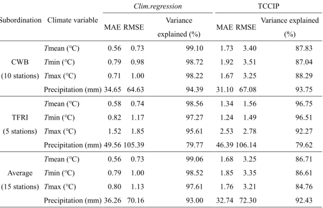
We collected historical records covering the period of 1961 to 2009 from 15 weather stations to evaluate the accuracies of clim.regression model. Ten of the 15 stations are subordinate to the Central Weather Bureau (CWB), which is the main corporation agency of TCCIP. The remaining five stations belong to the Taiwan Forestry Research Institute (TFRI), which is independent of the samples of TCCIP network. The observations from the 15 weather stations were also used to evaluate the magnitude of improvement over the original TCCIP gridded surfaces. Four sets of climate variable estimates generated by clim.regression, including monthly precipitation, monthly minimum temperature, monthly mean temperature and monthly maximum temperature, were evaluated against observations from the 15 weather stations (Table 2.3, Fig. 2.2). Prediction errors of clim.regression were assessed and compared using the following three statistical measures:
Mean error (ME):
where n is the number of samples, fi is the predicted value of the i-th sample and yi its real value.
Mean absolute error (MAE):
Root mean squared error (RMSE):
Table 2.3. Localities of 15 weather stations and the period of observed data that available for model evaluation.
Subordination/
Station Longitude Latitude Altitude (m) Observation period
Central Weather Bureau (CWB) Incorporated by TCCIP
Kaohsiung 120.32 22.57 2
1961–2009
Taitung 121.15 22.75 9
Hualien 121.61 23.98 16
Hengchun 120.75 22.00 22
Keelung 121.74 25.13 27
Taichung 120.68 24.15 84
Anbu 121.53 25.18 826
Sunmoon Lake 120.91 23.88 1,018
Alishan 120.81 23.51 2,413
Yushan 120.96 23.49 3,845
Taiwan Forestry Research Institute (TFRI) independent from TCCIP
Taimali 120.98 22.60 120 1980–2009
Liukuei 120.63 23.00 230 1999–2009
Fushan 121.60 24.76 634 1992–2003
Lienhuachih 120.90 23.93 666 1999–2009
Piluhsi 121.31 24.23 2,150 1991–2009
RESULTS
Scale-free climate surfaces from the downscaling model
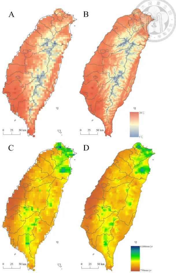
Clim.regression is a scale-free and topography-correspondent downscaling model, which attributes to the continuous and smooth characteristics of bilinear interpolation and the elevational adjustment by lapse rate from a dynamic local regression. Regular grids for MAT (mean annual temperature) and MAP (mean annual precipitation) surfaces were generated by the model at the spatial resolution of the original baseline data (5km × 5km) and a downscaled spatial resolution (250m × 250m) (Fig. 2.3). The results showed that MAT in Taiwan ranges from 1°C to 28°C and exhibits a trend of decline from lowland to
Fig. 2.2. Long-term observation data from fifteen weather stations were incorporated to evaluate the downscaling model. Solid stars demonstrate stations subordinate to the Central Weather Bureau of Taiwan (CWB). Open stars represent stations belonging to the Taiwan Forestry Research Institute (TFRI), which were independent from TCCIP system.
alpine and from south to north. A more detailed spatial distribution of temperature due to geographical effect, such as warm basin of Puli and cool tablelands of Linkou and Pagua, could also be revealed by the downscaled surface (Fig. 2.3A–B). The spatial distribution of MAP demonstrated a different pattern from that of MAT; it exhibited two-ended humid regions in the northeast and the southwest of Taiwan. The northeastern mountains in Taipei and Ilan and the southwestern edge of the Central Mountain Range in Kaohsiung and Pingtung are the moistest regions of Taiwan, and the downscaled surface more clearly revealed some precipitation hotspots with annual rainfall up to 6,000mm (Fig. 2.3C–D).
In comparison with the original climate dataset at the resolution of 5km × 5km, the downscaled one offers a detail depiction on the climatic alternation with topographies as the examples showed in Fig. 2.3. The scale-free modeling approach not only has the advantage in providing continuous and seamless climatic surface for large-scale studies (e.g., the classification of ecological-climatic regions, climatic niche modeling, and projections, etc.), but also generates accurate and point-specific climatic estimates as environmental correlates for plot-based researches (e.g., vegetation survey and plotting, etc.).
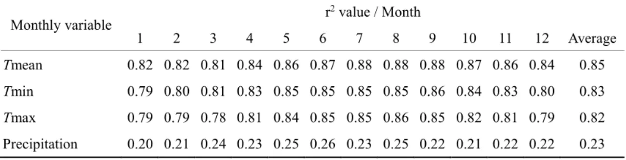
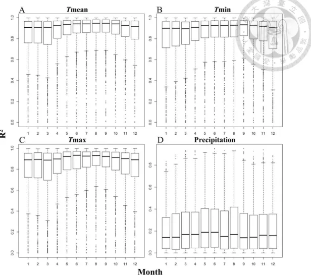
Table 2.4. The r-squared values of the local linear regressions for different monthly climate variables.
Monthly variable r2 value / Month
1 2 3 4 5 6 7 8 9 10 11 12 Average
Tmean 0.82 0.82 0.81 0.84 0.86 0.87 0.88 0.88 0.88 0.87 0.86 0.84 0.85 Tmin 0.79 0.80 0.81 0.83 0.85 0.85 0.85 0.85 0.86 0.84 0.83 0.80 0.83 Tmax 0.79 0.79 0.78 0.81 0.84 0.85 0.85 0.86 0.85 0.82 0.81 0.79 0.82 Precipitation 0.20 0.21 0.24 0.23 0.25 0.26 0.23 0.25 0.22 0.21 0.22 0.22 0.23
Fig. 2.3. Spatial distributions of mean annual temperature (MAT) and mean annual precipitation (MAP) for original climate data at the resolution of 5km and downscaled to the resolution of 250m. (A) Original and (B) downscaled MAT; (C) Original and (D) downscaled MAP. Data period: 1986–2005.
Lapse rate and effectiveness of the elevational adjustment
The dynamic local linear regression among the nine neighboring cells explained, on average, 85.3% of the total variation in monthly mean temperature. The amount of variance explained for monthly minimum temperature (83.1%) and monthly maximum temperature (81.9%) were slightly lower (Table 2.4). The average temperature lapse rate in the mountain areas was -5.65°C/km but displayed an obvious seasonal variation. Fig.
2.4A–C illustrate the same pattern in three primary temperature variables with a higher variation of lapse rate in winter (from Nov. to Apr.) than in summer (from May to Sep.).
The relationships revealed in the local regressions were weaker for precipitation than for temperatures. Only 20.3–25.7% of precipitation’s variation can be explained by the local regressions (Fig. 2.4D, Table 2.4).
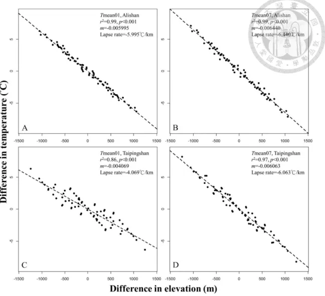
We compared the relationships between the changes in temperature and the elevation between two mountains, Alishan and Taipingshan. Such a relationship was stronger for Alishan with a steady lapse rate from -6.00 to -6.44°C/km from winter to summer. In contrast, a higher seasonal variation and a weaker relationship between temperature and elevation were observed in Taipingshan (Fig. 2.5).
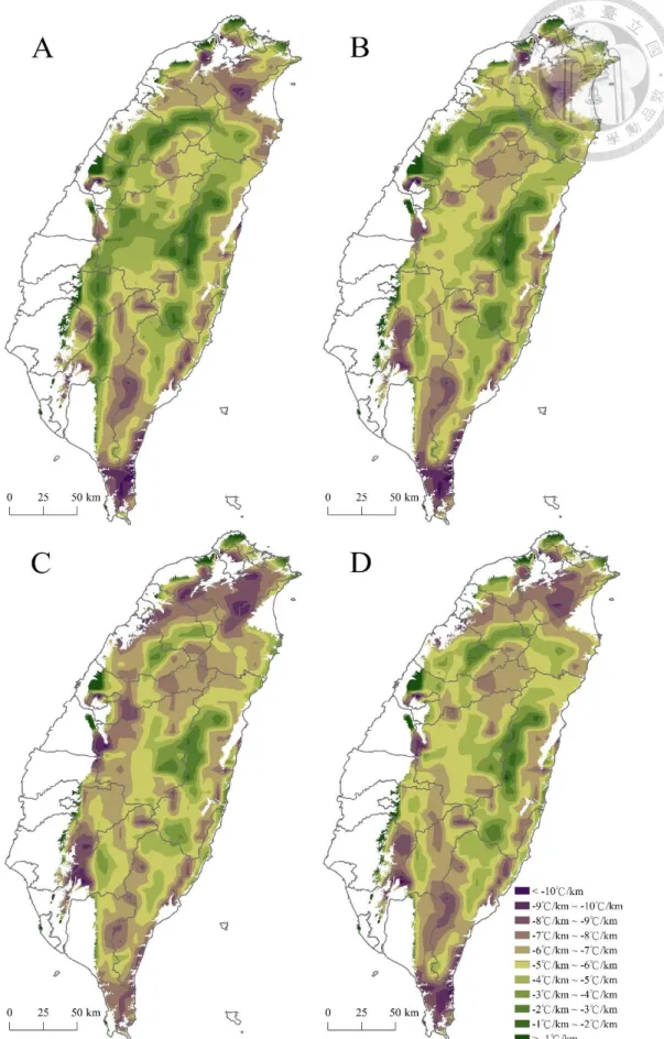
The spatial distributions of the estimated lapse rates varied among seasons and regions.
In winter, lower lapse rates for monthly average temperature (from -2 to -5°C/km) were exhibited in the central and western parts of the Central Mountain Range, especially in the hills from Hsinchu, Miaoli, Nantou, Chiayi to Kaohsiung. In contrast, very steep lapse rates (from -6 to -9°C/km) were demonstrated in the northeastern mountains and Hengchun peninsula (Fig. 2.6A). The spatial differentiation in lapse rate in most areas mitigated in summer, and demonstrated a mild geographical divergence with a range from
and Ilan, Hengchun peninsula, Tawu Mountain and the Costal Mountain Range, the steep lapse rates (<-6°C/km) could be found across all seasons of the year. Our dynamic local regression approach revealed the variation in the lapse rate both spatially and temporally over the island, and thus produced accurate adjustment for elevation.
Table 2.5. Summaries of statistical evaluations of clim.regression against historical observed data from Central Weather Bureau (CWB) and Taiwan Forestry Research Institute (TFRI).
Subordination Climate variable
Clim.regression TCCIP
MAE RMSE Variance
explained (%) MAE RMSE Variance explained (%)
CWB (10 stations)
Tmean (℃) 0.56 0.73 99.10 1.73 3.40 87.83
Tmin (℃) 0.79 0.98 98.72 1.92 3.51 87.04
Tmax (℃) 0.71 1.00 98.22 1.67 3.25 88.29
Precipitation (mm) 34.65 64.63 94.39 31.10 67.08 93.75
TFRI (5 stations)
Tmean (℃) 0.58 0.74 98.56 1.34 1.56 96.75
Tmin (℃) 0.82 1.17 97.27 1.24 1.49 96.51
Tmax (℃) 1.52 1.85 95.61 2.53 2.78 92.27
Precipitation (mm) 49.56 105.39 79.77 46.39 106.14 79.62
Average (15 stations)
Tmean (℃) 0.56 0.73 99.06 1.68 3.25 86.71
Tmin (℃) 0.79 1.00 98.52 1.85 3.35 86.61
Tmax (℃) 0.80 1.13 97.61 1.76 3.21 84.76
Precipitation (mm) 36.26 70.16 93.00 32.74 72.30 92.43
Fig. 2.4. Proportions of variance explained by local linear regressions in total variation among the nine neighboring cells for the four primary climate variables: (A) monthly mean temperature (Tmean), (B) monthly minimum temperature (Tmin), (C) monthly maximum temperature (Tmax) and (D) monthly precipitation, by month. The black horizontal solid lines inside the boxes indicate the medium. For temperature variables, a similar trend of higher variation in winter and lower variation in summer can be observed. Data period: 1961–
2009.
Fig. 2.5. Comparisons in lapse rates for winter and summer between two mountains, Alishan (A, B) and Taipingshan (C, D). Alishan (120.81E, 23.51N) is a mountain located in the south-west Taiwan, while Taipingshan (121.53E, 24.49N) is located in the north-east part. The two mountains have a similar elevation around 2,000m. Data period: 1961–2009.
Fig. 2.6. Spatial distributions of estimated lapse rate for monthly mean temperature in the mountain areas (regions higher than 100m asl) in Taiwan: (A) January, (B) April, (C) July and (D) October. Data period:
Statistical evaluations of the downscaling model and its improvement over TCCIP dataset The prediction accuracy of clim.regression was evaluated by comparing to historical observations from the 15 weather stations (Table 2.5). Clim.regression demonstrated a high prediction accuracy for monthly mean temperature with a low prediction error (0.56°C in MAE) and a high percent of variance explained (99.1%). The prediction accuracy and variance explanation were slightly lower for monthly minimum temperature and monthly maximum temperature in terms of the prediction error (0.79°C and 0.80°C) and the percent of variance explained (98.5% and 97.6%, respectively). However, the prediction accuracy was considerably lower for precipitation. The precipitation estimates explained 93.0% of the total variance of observations with a prediction error of 36.26mm in MAE.
Monthly mean temperature was the most predictable climate variable. The prediction accuracy of monthly mean temperature in regions lower than 2,500m asl could reach the level of 0.3–0.6°C in MAE. However, we found that the prediction error increased with elevation (r2=0.55, p=0.0015). For example, in the subalpine area of Taiwan, clim.regression had a comparatively weak predict ability with the MAE of 1.02°C.
Interestingly, such a relationship was not observed for monthly minimum temperature and monthly maximum temperature (r2=0.07 and 0.35, p=0.3252 and 0.0209). The prediction accuracy for precipitation was lower and accompanied with a higher variation and a less amount of variance explained (92.1%). In addition, there was no obvious trend found between prediction error in precipitation and altitude (r2=0.01, p=0.7612). It suggests that the pattern of precipitation could be dominantly influenced by regional terrains rather than a local elevational gradient within the 5km × 5km grids.
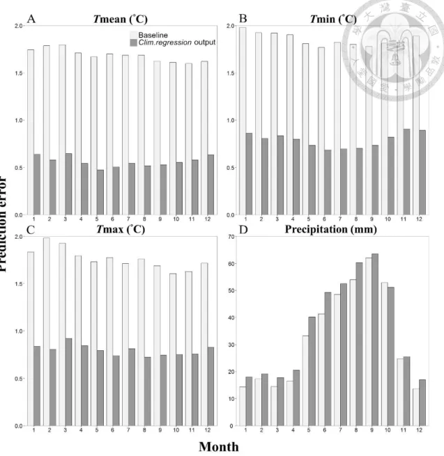
In comparisons to TCCIP original dataset, clim.regression reduced prediction errors by
1.12°C (66.7%), 1.06°C (52.3%) and 0.96°C (54.6%) for Tmean, Tmin and Tmax, respectively (Fig. 2.7A–C, Table 2.5). These results demonstrated that clim.regression effectively improved the accuracy and refined the spatial resolution of temperature estimates relative to the original dataset from TCCIP, especially with advantages in temperature projection for mountains with diverse topography. However, the improvement in precipitation is limited (Fig. 2.7D). Both TCCIP baseline and clim.regression had a higher prediction error for precipitation during summer months (May to Oct.). As illustrated in Fig. 2.8, the magnitude of the improvement was more substantial at higher elevations (the lower end of the temperatures), especially in the alpine area of Yushan (3,952 m) and Alishan (2,413 m). The downscaled temperatures followed a 1:1 relationship with observations much closer than the TCCIP predictions.
Fig. 2.7. Comparison in prediction error between baseline data (directly from TCCIP) and Clim.regression output of 15 weather stations for: (A) monthly mean temperature (Tmean), (B) monthly minimum temperature (Tmin), (C) monthly maximum temperature (Tmax) and (D) monthly precipitation.
Downscaling for future climate projections
Based on the estimated lapse rate of future scenarios, clim.regression was also effective to downscale the ‘gridded future climate data’ to a scale-free and continuous surface with the same 73 climate variables as for the historical period. Downscaled MAT by clim.regression for the reference period and future scenario in the mountainous area of Taiwan were illustrated in Fig. 2.9. The benefit of the downscaled MAT is clearly shown
in this example in term of fine spatial resolution and high topographical correspondence.
Based on the comparison among current and future climate under the RCP 4.5 scenario, not only an evident warming can be found in the valleys and plains but also demonstrate an obvious retreat of isothermals to the subalpine area (Fig. 2.9). Clim.regression has a solid advantage in generating current and future climate data with the same and desirable spatial resolution, which is a convenient for modeling biological response to climate change and for advanced comparative studies.
Fig. 2.8. An illustration to demonstrate the difference between observations from 15 weather stations and its corresponding climatic estimates from TCCIP outputs (red) and clim.regression in May for (A) monthly mean temperature (Tmean05), (B) monthly minimum temperature (Tmin05), (C) monthly maximum temperature (Tmax05) and (D) monthly precipitation (Precipitation05). It was clearly revealed that TCCIP outputs are biased as the decreasing of observed temperature, which is highly correspond to the raise of altitude.