使用單埠量測結果重建多埠電路之散射矩陣

國立臺灣大學電機資訊學院電信工程學研究所 博士論文

Graduate Institute of Communication Engineering College of Electrical Engineering ＆ Computer Science

National Taiwan University Doctoral Dissertation

使用單埠量測結果重建多埠電路之散射矩陣 Multiport S-matrix Reconstruction Using One-Port

Measurements

林沿鍾 Lin Yen-Chung

指導教授：瞿大雄 博士 Advisor: Chu Tah-Hsiung, Ph.D.

中華民國 104 年 6 月

June, 2015

誌謝

從碩士誌謝到博士誌謝，要感謝的人和事多了好多。寫論文的時候，總覺得

一頁的空間好長，而寫誌謝時卻又突然變得好短。但願有緣讀到這篇誌謝的大家，

能稍微感受到在這受限的文字背後，滿滿的感懷之意。

首先感謝最大力付出的瞿大雄教授，無論是實驗發想、技術乃至於文案，皆

得力於老師的扶持才有今天的成果。而在學術之外，當我在生活上遇到難題時，

瞿教授也盡力地協助，讓我更能穩定腳步。感謝季先生長年細心維持實驗室的正

常運作，把精良的設備隨時保持在最佳狀態，讓我在截稿的關鍵時刻能專注於實

驗內容，完全不用擔心儀器出狀況。感謝李偉強學長，雖然你不在實驗室已許久，

但在理論發想初期及初次投稿論文時，你的鼓勵跟建議讓我安心不少。感謝張祐

宸同學在重要時刻提供的實務技術指導。另外特別感謝我的電磁學啟蒙老師蔡智

明教授，在虛度了廿年之後，我才終於在您的課堂上首次從『學』窺見了『思』

的輪廓。得知您即將出任口試委員，也在我們這群大學同儕間引起一陣小騷動。

而能在您的認可之下取得學位對我更是意義非凡。

感謝家鄉父親的資助，母親的支持。隨著接觸的事物越來越多，才能體會過

去你們所維繫的穩定環境，對於一個人的影響有多麼巨大。感謝你們給過的那些

日子，遠超過任何物質所能代表。並期許我們都能有足夠的智慧與勇氣，面對未

來的任何挑戰。感謝大姊一家包括小愷替我分擔的憂慮。當我正在與論文水深火

熱又面臨研發替代役的抉擇時，謝謝你們耐心地替我緩解心裡的不安。當然我也

不會忘記耘樂跟牧澄這兩顆小蘿蔔帶給大家的歡樂（！？），未來還請不要吝嗇地

放下身段，無下限地賣萌吧！感謝林士恆在我最支不開身的時候，一肩負起照顧

爸爸的責任。我一定要告訴你當我知道你要返回嘉義時，焦頭爛額的我是鬆了多

麼大的一口氣。感謝堅不可摧 364 聯盟的蘇聖琪，林昱廷以及最接近第一線看我

火燒屁股並且提供關鍵技術支援的黃品澄。感謝我的蘇曉芸，妳的一切決定都只

為了成就我的里程碑。只要是為了學業，對於我的任何提議一定是說一不二全力

配合，到了研究後期更是大量仰賴妳的資助。而當我的研究有了新的進展，妳就

靜靜地聽我興奮的轉述。除了老師之外，就只有妳看著我把理論一層層建築起來，

妳就是那位跟我併肩衝鋒的人。感謝蘇曉洳和蘇聖凱，謝謝你們過去十年來給了

我這麼特別的回憶，從五月天、皮克斯、新台灣原味、555、廈門、上海到龜山島，

無論到哪裡都留下了我們的足跡，大家合作把媽媽嚇到眼鏡噴發的那一天更是我

們慶生成就的顛峰！是你們三姊弟一起把笑聲倒進我的生活裡。最後，謹以無限

追思緬懷無緣見到此刻的長輩。我想我是少數能吃著岳母準備的便當做著研究的

幸運兒，雖然只差一點，妳就能看到這一切，但我相信妳一定很驕傲妳的女婿終

於順利完成了這個階段。願您在坎坷的一生之後能安息。謹將此微薄榮耀獻予您，

以及所有我深切在乎的大家。

i

摘要

本論文提出以多個單埠之散射參數量測，據以重建多埠被動及主動電路之散

射矩陣。降埠法係使用埠數少於 n 埠之網路分析儀，以獲得一 n 埠電路之散射矩

陣，已知適用降埠法之網路分析儀埠數，最少為雙埠或三埠，本論文則將埠數進

一步降至單埠，即最低埠數。

第二章闡述對一雙埠電路，如何使用輔助電路及單埠終端器，由多個單埠散

射參數，重建該雙埠電路之散射矩陣。其重建結果進一步應用於降埠法，由多個

單埠散射參數量測值，重建 n 埠電路之散射矩陣。由於使用單埠終端器，對於主

動電路可能造成振盪，因此本章亦敘述雙埠主動電路之散射矩陣重建方法。最後，

對於多埠互易電路，則提出可不使用降埠法，重建其 n 埠散射矩陣。

由於輔助電路在降低量測埠數至單埠極為重要，第三章則討論輔助電路之影

響，藉由適當選擇輔助電路，可降低單埠量測實驗數目，減低重建時數值運算之

困難，以及增加重建結果之準確性。

第四章則敘述四個實驗實例。包含三埠被動互易電路，三埠被動非互易電路

以及雙埠主動電路。重建結果與直接散射矩陣量測結果比較，顯示其一致性，重

建誤差亦予以討論。

關鍵字-多埠電路, 散射矩陣量測

ii

Abstract

In this dissertation, study results to reconstruct the scattering matrix (S-matrix) of a

multiport network from a set of one-port scattering parameter (S-parameter)

measurements are presented. Port reduction method (PRM) is a method to acquire the

S-matrix of an n-port network by using a reduced port vector network analyzer (VNA).

PRMs have shown that the minimum number of port of a VNA is two or three. This

study attempts to go one step further to reduce the number of port to be one, which is

the lowest number.

In Chapter 2, reconstruction method using auxiliary circuits and one-port

terminations to solve the S-matrix of a two-port network is described. The type-II PRM

is then applied to the results for the reconstruction of the S-matrix of an n-port network.

Since the terminations used in one-port measurement may cause an active network

oscillation. Further development on reconstructing a two-port active network is given.

Finally, the method in reconstructing the S-matrix of a multiport reciprocal network

without using PRM is also presented.

The use of auxiliary circuits plays an important role in reducing the number of

measured port to be one. The effects of the auxiliary circuits are discussed in Chapter 3.

By properly selecting the auxiliary circuit, one can reduce the number of one-port

iii

measurements, ease the problem encountered in the reconstruction, and increase the

accuracy of the reconstructed results.

Chapter 4 presents four experimental examples to verify the developed

reconstruction methods. They include a three-port reciprocal network, a passive

nonreciprocal network and a two-port active network. The reconstructed results are

compared with the directly measured S-matrices. They are shown in good agreement.

Errors of reconstructed results are also discussed.

keywords: Multiport network, scattering matrix measurement

iv

Contents

摘要

Abstract

Contents

Chapter 1 Introduction

1.1 Multiport network S-matrix measurement ... 1

1.2 Reconstruction methods ... 2

1.3 Port reduction methods ... 2

1.4 Motivation and contribution ... 3

1.5 Chapter outline ... 5

Chapter 2 Formulation

2.1 Two-port network ... 10

2.1.1 Diagonal elements ... 10

2.1.2 Off-diagonal elements... 12

2.2 Two-port active network ... 14

2.3 Reciprocal network using comparison process ... 16

v

2.3.1 Formulation ... 17

2.3.2 Three-port case ... 18

2.4 Summary ... 22

Chapter 3 Selection of auxiliary circuit

26

3.1 Two-port network

26

3.2 Two-port active network

28

3.3 Two-port reciprocal network

29

3.4 Summary

31

Chapter 4 Experimental results

4.1 Three-port reciprocal network

33

4.2 Three-port nonreciprocal network

38

4.3 Two-port active network

39

4.4 Three-port reciprocal network using comparison process

41

4.5 Summary

42

Chapter 5 Conclusion

Appendices

vi

Appendix A Prove of q p / = − ( S

+ S

)

73 Appendix B Prove of r p / = S S

73

References

1

Chapter 1 Introduction

1.1 Multiport network scattering matrix measurement

The scattering matrix (S-matrix) of a multiport network can be acquired from the direct measurement using a full port vector network analyzer (VNA), or from multiple

measurements with the use of a reduced port VNA and proper reconstruction methods

[1]-[9]. The former is a straight forward approach. However, the necessary multiport

VNA is usually costly and requires complicated calibration [10]-[12] due to the large

number of error terms and error paths [11]. In some situations, the multiport calibration

can be simplified by ignoring the leakage between each port [13]. As for the situation of

non-negligible leakage such as the on-wafer MMIC multiport measurement, Ferrero and

Sanpiertro proposed a calibration method [14] to take these leakages into account. In

[14], one needs to perform 5 calibration steps to obtain 35 linear equations to solve all

the error terms of a leaky three-port VNA.

The alternative approach to obtain the S-matrix of a multiport device-under-test

(DUT) is to use a reduced port VNA and certain known terminations. It can characterize

a multiport network with less expensive equipments and ease the consideration of

calibration. However, the accuracy of results using these approaches would be affected

by the numerical issue of the reconstruction algorithm [5], [8], [15], the numerous

reconnections during the measurement and the confidence in those known terminations.

2

Ideally, one can use perfect terminations and a reduced port VNA to complete a

multiport measurement based on the definition of S-matrix. However, a perfect

termination is impractical and the imperfect effect must be taken into account. Rigorous

works of this issue have been proposed for decades. These methods using reduced port

VNA can be categorized into two types, which are direct reconstruction methods and

port reduction methods (PRMs). They will be discussed in the following two sections.

1.2 Reconstruction methods

Since a multiport VNA was not as commercially available in early days, some

rigorous works [2]-[5] proposed approaches to obtain the S-matrix of a multiport DUT

using a two-port VNA. These approaches have led to build a four-port measurement

system using a two-port VNA and switches [6]. The formula of these approaches to

reconstruct the S-matrix of a multiport DUT is based on matrices manipulation.

Associated researches in easing the requirement of known terminations [16] and in

accuracy analyzing [15] have also been presented. The concept of condition number is

used in [15]-[16] to explain how the terminations and the DUT affect the accuracy of

results. Such accuracy analysis is complicated and difficult because the matrix

manipulation used in these direct reconstruction methods are inherently abstract.

1.3 Port reduction methods

On the other hand, [7] provides a different point-of-view in reconstructing an

3

n-port S-matrix. This method reduces the number of measured ports by one by

connecting a known termination to the unmeasured port. The n-port S-matrix is then

reconstructed from a set of reduced (n-1)-port measured S-matrices. This PRM is

continued until it fails or reaches a port order at which a VNA is available. Three types

of PRMs are proposed in [8]-[9]. Reducing one port at a time simplifies the

reconstruction problem. The accuracy issue is therefore simpler [8] than that of direct

reconstruction methods and can be discussed in a physical sense.

1.4 Motivation and contribution

Among the reduced port methods, the reconstruction methods in [1]-[5] can reduce

the number of measured ports to two ports. Take the method presented in [5] as an

example. The reconstructed n-port S-matrix can be calculated from (10) in [5] given as

1 1

S =Γ -Σ^{− −} (1.1)

where

Γ

coefficients of the known terminations. The temporary matrix

Σ

reflection coefficients of the known terminations and the reduced port measured data.

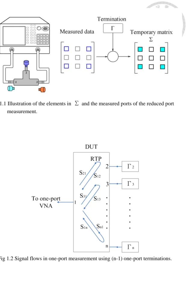
The measured ports of the reduced port measurement determine which elements in

Σ

can be calculated as shown in Fig. 1.1. The calculated elements in

Σ

symmetric to the diagonal line. Therefore, the off-diagonal elements will not be

calculated if only one-port measurement is performed.

4

On the other hand, (5) and (6) in [8] given as

(

)

1 2 1 2

( ) ( )

( ) ( )

1 1 n n ijⁿ ijⁿ

ij ij ij nn

n n n n

S S

S S S S

 

− + − = −

 

Γ Γ  Γ Γ (1.2)

(

)

1 3 1 3

( ) ( )

( ) ( )

1 1 n n ijⁿ ijⁿ

ij ij ij nn

n n n n

S S

S S S S

 

− + − = −

 

Γ Γ  Γ Γ (1.3)

imply that the VNA used in applying the type-I PRM should have at least two ports to

obtain Sij^{( )n} . Otherwise, only the diagonal elements of the S-matrix of the DUT can be

solved. Similar restriction can be observed in the type-II PRM [8]. The VNA must have

at least two ports to get the measured data Sin⁽ⁿ⁻¹⁾ which appears in (16) of [8]. As for

the type-III PRM, the condition i≠ stated in (8) of [9] clearly points that the type-III j

PRM is not suitable for one-port VNA. In fact, the type-III PRM could reduce the

number of measured ports to two ports for reciprocal circuits or three ports for

nonreciprocal circuits.

Conventionally, it is believed that the reconstruction by reducing the measured

ports to one port is quite difficult because the forward transmission coefficient always

multiplies with the backward transmission coefficient in a round trip path (RTP) to be

defined later. Fig 1.2 illustrates the problem in reducing the minimum number of

measured port to be one by using (n-1) one-port terminations. To solve this problem, an

auxiliary circuit is proposed in this study to provide additional signal paths as shown in

Fig 1.3 by taking a two-port DUT as an example. Such an arrangement will give the

5

one-port measured data of the VNA contains more information of the RTP, and make it

possible to separate the forward and reverse transmission coefficients of the DUT.

One-port VNA or six-port reflectometer has been available for years [17]. It is

much simpler in operation and less expensive than two-port and multiport VNAs. The

use of one-port VNAs can perform measurements of the insertion loss and the distance

to the fault of a cable and the reflection coefficient of a one-port DUT. Recently, USB

based one-port VNAs, such as Anritsu MS46121A and Copper Mountain Technologies

R54, are available. These then lead to this study of reducing the measured ports of a

multiport DUT to the minimum number to be one and acquiring its multiport S-matrix

in a cost-effective manner. Extending the operating frequency to the THz range,

one-port VNA can further ease the implementation difficulty of a sub-mmw multiport

VNA.

1.5 Chapter outline

Since the reduced port methods [1]-[9] can be applied to reduce the measured ports

to two ports, Chapter 2 mainly describes the formulation of acquiring the S-matrix of a

two-port DUT from one-port measurements with the use of an auxiliary circuit. The

formulation in dealing with the two-port DUT, including reciprocal and nonreciprocal,

is presented in Section. 2.1. The modified formulation for a two-port active network is

described in Section 2.2. Section 2.3 then describes an alternative method to determine

6

the S-matrix of a reciprocal DUT through a comparison process. By using this process,

one can characterize an n-port reciprocal DUT without using the reduced port methods

[1]-[9].

Chapter 3 describes the selection of auxiliary circuit. To reconstruct the S-matrix of

a two-port DUT, the number of one-port measurements in this study is five, which is in

excess of that of unknowns by one. However, for certain two-port nonreciprocal

networks such as isolator or amplifier as described in Section 3.1, one can properly

select the auxiliary circuit to reduce the number of measurements to four to be equal to

the number of unknowns. Section 3.2 then gives the criteria of auxiliary circuit in

characterizing a two-port active DUT. The effect of the selection of the auxiliary circuit

on the accuracy of the reconstructed results is discussed in Section 3.3 for a two-port

reciprocal DUT.

Chapter 4 presents four experimental results of reciprocal and nonreciprocal DUTs.

Three-port reciprocal and nonreciprocal examples are given in Section 4.1 and Section

4.2, respectively. In each example, the type-II PRM [8] is applied to reconstruct the

three-port S-matrix from two-port results. The reconstruction of two-port S-matrix from

one-port measurements is performed using the formulation to be presented in Section

2.1. The reason to use the type-II PRM rather than the type-I [8] or the type-III PRM [9]

is based on the fact that fewer one-port measurements are involved. Section 4.3 shows

7

the results of a two-port active DUT, while Section 4.4 shows the results of a three-port

reciprocal DUT by using comparison process. Finally, a conclusion is given in Chapter

5.

8

Fig 1.2 Signal flows in one-port measurement using (n-1) one-port terminations.

Fig 1.1 Illustration of the elements in

Σ

9

Fig 1.3 Assembly of auxiliary circuit and DUT.

10

Chapter 2 Formulation

This chapter describes the formulation of solving the S-matrix of a two-port DUT from a set of one-port measurements. Section 2.1 presents the formulation of a two-port

DUT. Section 2.2 then modifies the formulation to the case of a two-port active DUT.

One can then apply PRMs to the two-port results to reconstruct the S-matrix of an n-port

DUT. In Section 2.3, by applying the symmetry property of a reciprocal DUT, one can

find the S-matrix of an n-port reciprocal DUT through a comparison process [18]

without using the reduced port methods [1]-[9].

2.1 Two-port network

In this section, the formulation of solving the diagonal elements of a two-port

S-matrix from one-port measurements is given in Section 2.1.1. The formulation of

solving the off-diagonal elements with the use of auxiliary circuits is then given in

Section 2.1.2.

2.1.1 Diagonal elements

The reflection coefficient at port 1 of a two-port DUT by terminating its port 2 with

Γ2 is given by

12 21 2 (2)

11 11

22 2

1 S S S S

= + S

− Γ

Γ (2.1) or

(2) (2)

11 11 2 22 2( 12 21 11 22) 11

S +S ΓS +Γ S S −S S =S . (2.2)

11

The superscript of S₁₁^{( 2)} denotes that the terminated port is port 2. Similarly, by

terminating port 1 with Γ1, one can obtain the following equation for port 2

(1) (1)

22 22 1 11 1( 12 21 11 22) 22

S +S ΓS +Γ S S −S S =S . (2.3)

From (2.2) and (2.3), one may find that with the help of three known terminations,

for example, Γ2 a, Γ2b, and Γ1a, the three unknowns of S11, S22 and S S12 21−S S11 22

could be solved. After that, one can obtain S S12 21 by substituting the solved S11 and

S22 into (2.2) or (2.3). Therefore, from three one-port measurements of a two-port DUT by terminating the other port with three different known terminations, one can

solve the diagonal elements S11 and S22 and the RTP term S S12 21≡RTP through

the following matrix equation

(2 ) (2 )

2 2 11

11 11

(2 ) (2 )

2 2 22

11 11

(1 ) (1 )

1 1 11 22

22 22

1 1

1

a a

a a

b b

b b

a a

a a

S S S

S S S

S RTP S S S

     

    = 

     

   −   

   

Γ Γ

Γ Γ

Γ Γ

. (2.4)

In the above procedure, one sequentially connects two terminations at port 2 and

one termination at port 1 of DUT to solve the diagonal elements. Note, the diagonal

elements can also be solved if all the three terminations are sequentially connected at

port 1 or port 2. However, (2.4) is recommended for the consideration of accuracy.

Considering (2.1), corresponding to the case of connecting Γ at port 2, ₂ S is an ₁₁

individual unknown term while S is embedded in the denominator. The sensitivities ₂₂

of solving S and ₁₁ S are different. Further experimental results indicate that by ₂₂

12

connecting one termination at one port and two terminations at the other port, the

accuracy of one diagonal element becomes slightly worse and the other one is

dramatically improved.

Note the RTP term in (2.4) is a multiplication of the forward transmission

coefficient S21 and the reverse transmission coefficient S12. Hence, the separation of

S21 and S12 needs additional measurements using an auxiliary circuit to be discussed Section 2.1.2.

2.1.2 Off-diagonal elements

In Fig. 1.3, a three-port auxiliary circuit is used to separate the RTP term in (2.4).

The three ports of the auxiliary circuit are denoted as P1, P2 and P3. Its S-matrix is

known and given by A whose elements are aij with i , j =1, 2, 3. Note that the

auxiliary circuit needs advance characterization using a three-port VNA.

As shown in Fig. 1.3, port P1 is connected to a VNA for one-port measurement.

Ports 1 and 2 of the DUT are connected to ports P2 and P3 of the auxiliary circuit.

The measured reflection coefficient Γ at port m P1 is given as [5]

Γm = A^II +A S I^IJ [ −A S^JJ ]⁻¹A^JI

.

In (2.5) S is a two-port S-matrix of the DUT, I is a unit matrix, and the remaining

matrices related to the auxiliary circuit are given by

13

 

=  

 

II IJ

JI JJ

A A A A A

11 12 13

21 22 23

31 32 33

a a a

a a a

a a a

 

 

=  

 

 

.

By substituting (2.6) into (2.5), it can be explicitly expressed as

0 1 12 2 21

11

0 1 12 2 21

m

N N S N S

a B

D DS D S

+ +

− = ≡

+ +

Γ (2.7)

where

0 12 21 11 13 31 22

N =a a S +a a S

12 23 31 13 32 21 12 21 33 13 31 22 11 22

(a a a a a a a a a a a a )S S

+ + − −

12 21 33 13 31 22 12 31 23 13 32 21 12 21

(a a a a a a a a a a a a )S S

+ + − −

1 12 31

N =a a (2.8)

2 13 21

N =a a

and

0 1 22 11 33 22 ( 22 33 23 32) 11 22

D = −a S −a S + a a −a a S S +(a a23 32−a a22 33)S S12 21

1 32

D = − (2.9) a

2 23

D = − . a

One can further express S12 as

12 21

S RTP

= S (2.10) and rewrite (2.7) as a quadratic equation of S21 given by

2

2 2 21 0 0 21 1 1

(N −BD S) +(N −BD S) +(N −BD RTP) =0. (2.11) As the auxiliary circuit is properly characterized, all aij are known. By using the

known aij and S11, S22 and RTP solved from (2.4), one can then solve S21.

However, there are two solutions of S21 from (2.11). An additional one-port

14

measurement with the use of another auxiliary circuit is needed to solve another set of

two solutions of S21. These two sets then have the correct S21 in common. Once the

correct S21 is found, S12 can be calculated using (2.10).

In general, there are a total of five one-port measurements involved to reconstruct

the S-matrix of a two-port DUT. Three one-port measurements are used to solve the

diagonal elements S11 and S22 and RTP term as described in Section 2.1.1. In

Section 2.1.2, two additional one-port measurements are performed with the use of two

auxiliary circuits to solve the off-diagonal elements S21 and S12.

For a reciprocal two-port DUT, by applying S12 =S21 in (2.7), it becomes a linear

equation given by

0 1 2 21

11

0 1 2 21

( )

( )

m

N N N S

a D D D S

+ +

− =

+ +

Γ (2.12)

to solve S21 accordingly. Therefore, four one-port measurements are sufficient to

reconstruct the S-matrix of a reciprocal two-port DUT.

Note that for a reciprocal two-port DUT (2.10) can be written as

2

S21 =RTP. (2.13) The square root of RTP gives the sign ambiguity of S21 as discussed in [18],

however, (2.12) can solve S21 directly.

2.2 Two-port active network

In Section 2.1.1, a one-port termination is connected on the unmeasured DUT port

15

to solve the diagonal terms. This connection may cause possible oscillation or damage

the DUT as the two-port DUT is active. An alternative approach is then developed

without using one-port terminations. Instead, five auxiliary circuits are used to perform

five one-port measurements.

Since three one-port terminations in Section 2.1 are not used, the diagonal

elements become unknowns. Rewrite N0 in (2.8) as

0 a 11 b 22 c( 11 22 12 21)

N = N S +N S +N S S −S S (2.14) where

12 21

Na =a a

13 31

Nb=a a (2.15)

12 23 31 13 32 21 12 21 33 13 31 22.

Nc=a a a +a a a −a a a −a a a Similarly, D0 in (2.9) is rewritten as

0 1 a 11 b 22 c( 11 22 12 21)

D = +D S +D S +D S S −S S (2.16) where

22

Da = −a

33

Db = −a (2.17)

22 33 23 32

Dc =a a −a a By substituting (2.14) and (2.16) into (2.7), one can obtain a linear equation as

11 22 1 1 12 2 2 21 det

(Na −BD Sa) +(Nb−BD Sb) +(N −BD S) +(N −BD S) +(Nc−BD Sc) =B

(2.18)

where

det 11 22 12 21.

S =S S −S S (2.19)

Note there are five unknowns, S11, S22, S12, S21, and Sdet, in (2.18). All the

16

coefficients and constant term in (2.18) are related to the S-matrix of auxiliary circuit

and measured data. Therefore, one can solve these five unknowns through five one-port

measurements with the use of five different auxiliary circuits.

2.3 Reciprocal network using comparison process

This section describes a method to obtain the S-matrix of an n-port reciprocal DUT

without using the reduced port methods [1]-[9]. At first, the diagonal elements of the

n-port S-matrix and the RTP terms will be solved. By applying the symmetric property

of the S-matrix of a reciprocal DUT, the off-diagonal elements can then be solved by

directly taking square root of the RTP terms. However, this will result in several

possible S-matrices, and it will encounter an ambiguity problem in selecting the correct

one. To solve this, additional one-port measurements are performed with the use of a

characterized (n-1)-port auxiliary circuit. On the other hand, by applying the S-matrix of

the auxiliary circuit and all the possible S-matrices, one can calculate all the possible

one-port measured values according to the assembly of the DUT and the auxiliary

circuit. These calculated results are then compared with the one-port measured results.

The comparison results will then determine the correct S-matrix.

The formulation and the concept of solving the RTP terms and the diagonal

elements of the S-matrix of a reciprocal DUT is described in Section 2.3.1. The method

in finding the correct S-matrix and the way to reduce the number of one-port

17

measurements is described with a three-port DUT case as shown in Section 2.3.2.

2.3.1 Formulation

This section starts with (2.1) and a three-port DUT which its port 3 is terminated

with a termination. After the explanation of the notation and the introduction of the

formulation, the solution will then extend to an n-port DUT case.

Since a three-port DUT can be regarded as a two-port network if one of its port is

terminated, the method in Section 2.1.1 to solve the reflection coefficients and the RTP

term of a two-port network still stands in this case. However, the terms in (2.1) needs to

be modified to show the difference between a two-port DUT and a three-port DUT. The

modified equation of (2.1) is given as

(3) (3)

(3,2) (3) 12 21 2

11 11 (3)

22 2

1 S S S S

= + S

− Γ

Γ (2.20)

The term S₁₁^(3,2) is the reflection coefficient measured at port 1 of the DUT with its port

3 and port 2 are terminated with terminations. The superscript denotes the port or ports that are terminated with known terminations. From (2.20), one can solve S₁₁⁽³⁾, S₂₂⁽³⁾

and S₁₂⁽³⁾S₂₁⁽³⁾ with the use of three terminations Γ2 a, Γ2b, and Γ2 c. After that, since

the intermediate parameter S₁₁⁽³⁾ is composed as

13 31 3 (3)

11 11

33 3

1 S S S S

= + S

− Γ

Γ , (2.21) the reflection coefficients and the RTP term of the three-port DUT, e.g. S11, S33, and

18

13 31

S S , can be solved with the use of three terminations Γ3a, Γ3b, and Γ3c.

The above procedure shows two things that should be noticed. The first is that the intermediate RTP terms such as S₁₂⁽³⁾S₂₁⁽³⁾ are helpless in solving the S-parameters of

the next higher order in port number. The other is that the number of measurements to

solve the diagonal elements of an n-port DUT is theoretically 3⁽ⁿ⁻¹⁾.

To extend to an n-port DUT, (2.20) can be rewritten as

( , 1,...,3) ( , 1,...,3)

( , 1,...,3,2) ( , 1,...,3) 12 21 2

11 11 ( , 1,...,3)

22 2

1

n n n n

n n n n

n n

S S

S S

S

− −

− −

= + −

−

Γ

Γ . (2.22)

From (2.22), it is clear that with three terminations placed in sequence, one can find

some of the intermediate parameters of the higher order in port number. A general form

of (2.22) is shown below, which could help finding the arbitrary intermediate

parameters. It is given as

( , 1,..., 1, 1,...) ( , 1,..., 1, 1,...) ( , 1,..., 1, , 1,...) ( , 1,..., 1, 1,...)

( , 1,..., 1, 1,...)

1

n n k k n n k k

n n k k k n n k k ik ki k

ii ii n n k k

kk k

S S

S S

S

− + − − + −

− + − − + −

− + −

= +

−

Γ

Γ . (2.23)

2.3.2 Three-port case

Section 2.3.1 has described the method in finding the RTP terms and the diagonal

elements of the S-matrix of an n-port reciprocal DUT. This section will use a three-port

reciprocal DUT as a specific example to demonstrate how to find the off-diagonal

elements. Furthermore, by properly choosing the terminated port of the DUT and

arranging the one-port measurements, the number of one-port measurements can be

19

reduced to be less than 3⁽ⁿ⁻¹⁾.

At first, a generalized form of (2.1) can be expressed as

( )

1

ij ji j j

ii ii

jj j

S S S S

= + S

− Γ

Γ ^. (2.24)

Consider a three-port reciprocal DUT with its port 3 is terminated with Γ3a, (2.20) can

be rewritten as

(3 ) (3 )

(3 ,2) (3 ) 12 21 2

11 11 (3 )

22 2

1

a a

a a

a

S S

S S

= + S

−

Γ

Γ (2.25)

and (2.4) becomes

(3 ,2 ) (3 ) (3 ,2 )

11 2 2 11 11

(3 ,2 ) (3 ) (3 ,2 )

11 2 2 22 11

(3 ,1 ) (3 ) (3 ) (3 ) (3 ) (3 ,1 )

22 1 1 12 21 11 22 22

1 1

1

a a a a a

a a

a b a a b

b b

a a a a a a a a

a a

S S S

S S S

S S S S S S

     

     

    = 

   −   

     

Γ Γ

Γ Γ

Γ Γ

. (2.26)

With the help of (2.26), one can solve the two intermediate parameters S₁₁^{(3 )a} and S₂₂^{(3 )a} .

Another two intermediate parameters S₁₁^{(3 )b} and S₂₂^{(3 )b} can also be solved from (2.26)

by simply replacing Γ3a with Γ3b. Similarly, the last two parameters S₂₂^{(1 )a} and

(1 ) 33

S a could be solved by terminating the port 1 of a three-port DUT with Γ1a. The

necessary one-port measurements are summarized in Table 2.1 (a). In this table the

corresponding one-port measurement of S₁₁^{(3 ,2 )a a} , for example, is denoted as “1_3a2a”.

The notation “*” marks the repeated measurement.

20

As described in Table 2.1 (a), six intermediate parameters are solved accordingly.

One can then use these intermediate parameters to find all the possible S-parameters of

the three-port DUT in the following three steps.

In the first step, one may solve S and ₁₁ S by replacing all the 2’s in (2.4) with ₃₃

3’s based on the three intermediate parameters of S₁₁^(3a), S₁₁^(3b) and S₃₃^(1a). In addition,

one can also obtain S S by substituting _{13 31} S and ₁₁ S into the expression of ₃₃

13 31 11 33

S S −S S . Therefore, in this step, S , ₁₁ S and ₃₃ S S are solved as illustrated in _{13 31}

the first row of Table 2.1 (b).

In the second step, one can use the intermediate parameters S₂₂^(3a) and S₂₂^(3b) with

the case ( , )i j =(2,3) in (2.24) to write the corresponding matrix equation. Since S ₃₃

is solved already, one can solve the unknowns of S and ₂₂ S S using (2.27) as _{23 32}

illustrated in the second row of Table 2.1 (b).

(3 ) (3 )

3 22 22 22 3 33

(3 ) (3 )

3 23 32 22 22 3 33

1 .

1

a a

a a

b b

b a

S S S S

S S S S S

 − 

   

=  

    −

     

Γ Γ

Γ Γ (2.27)

In the last step, one can then calculate S S by using the intermediate parameter _{12 21}

) 1 ( 22

S a with (2.24) as

(1 )

22 22 11 1

12 21 1

( ^a )(1 _a)

a

S S S

− − Γ =S S

Γ (2.28)

in which S and ₁₁ S are already solved. This step is illustrated in the third row of ₂₂

Table 2.1 (b).

21

Table 2.1 (b) then summarizes the procedures given above. The notation “**”

marks the parameters already solved in the second step. The solved results in Table 2.1

(b) include the three diagonal elements. As for the off-diagonal elements, because the

three-port DUT is reciprocal, one can simply take the square root of the solved results of

12 21

S S , S S and _{13 31} S S . However, this would yield two possible values which are _{23 32}

180^o apart for each term. If we use “+” and “-” to denote the solution in the upper half and lower half complex plane, there are eight configurations for (S ,₁₂ S ,₁₃ S ) with ₂₃

ambiguities from (+, +, +) to (-, -, -).

To separate the off-diagonal S-parameters apart, one needs additional one-port

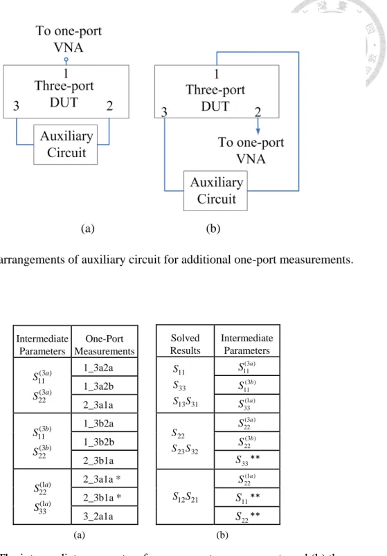
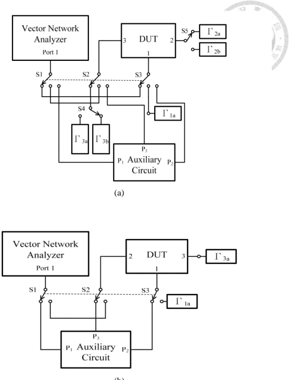
measurement as shown in Fig. 2.1. According to the assembly in Fig. 2.1(a), the DUT

port 2 and port 3 are connected to a known two-port auxiliary circuit. It then may give

signal paths not containing the RTP. Such paths can then be used to avoid the self

multiplication terms.

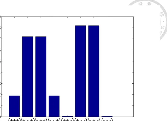
To achieve this, all the eight configurations are firstly listed, then the S-matrix of

the auxiliary circuit is applied to calculate the eight reflection coefficients according to

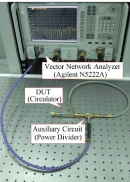
the arrangement of Fig 2.1 (a). Experimental study to be presented in Section 4.4 for an

Agilent 11667B power splitter is used as a three-port reciprocal DUT. By comparing the

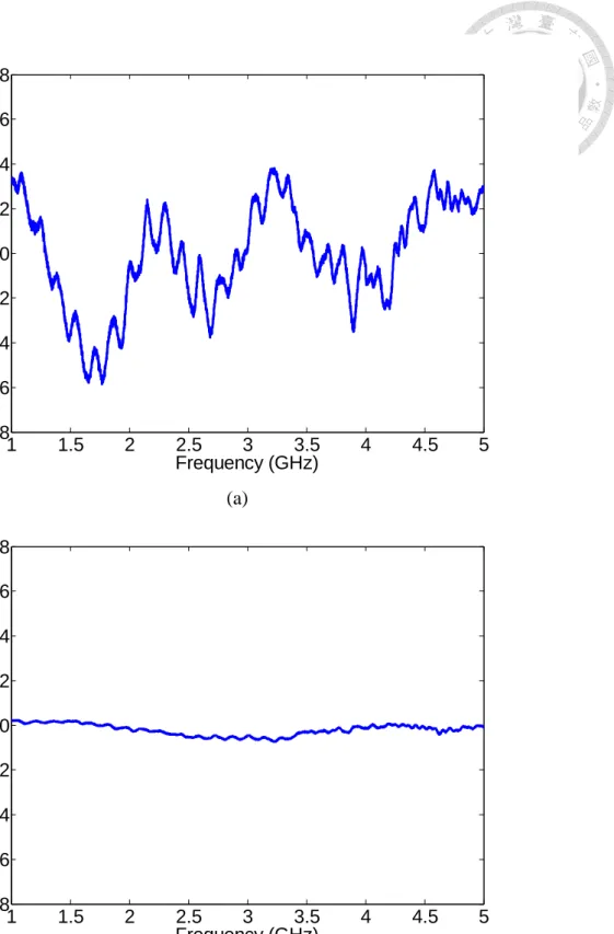
calculated and measured reflection coefficients, there are six configurations showing the

inconsistence as illustrated in Fig. 2.2. The vertical axis of Fig. 2.2 shows the distance

22

of the measured and calculated reflection coefficients defined as

Calculated Measured

Distance =Γ −Γ (2.29)

where “Γ” denotes the reflection coefficient. As for the remainder 2 configurations of

(+, +, -) and (-, -, -), another one-port measurement as shown in Fig 2.1 (b) is performed

to help selecting the correct one. Reconstructed results will be given in Section 4.4.

2.4 Summary

The formulations in reconstructing the S-matrix of a two-port network or an n-port

reciprocal network are presented in this chapter. To reduce the possibility of damaging

the DUT, the experimental procedure and the formulations for active devices are

modified. Generally speaking, the auxiliary circuits are required to be fully known.

However, the requirement of the auxiliary circuits used in the comparison process given

in Section 2.3 can be relaxed. Since the possible off-diagonal elements obtained in the

comparison process are 180^o apart, a rough knowledge of the auxiliary circuits is

sufficient to determine the correct S-parameters.

Note that reconstruction methods in [8] and [9] use redundant equations to solve

the reflection coefficients of certain terminations. This then leads the terminations can

be partially unknown. However, in the one-port measurement case presented in this

chapter, only one equation is available in each one-port measurement. It is then difficult

23

to have redundant equations to make the auxiliary circuit partially known.

24

Fig. 2.1 Two arrangements of auxiliary circuit for additional one-port measurements.

Table 2.1 (a) The intermediate parameters from one-port measurements and (b) the intermediate parameters for solving the results.

Solved Results

Intermediate Parameters

31 13 33 11

S S S

S 11⁽³⁾

S a ) 3 ( 11

S b ) 1 ( 33

S a

32 23 22

S S S

) 3 ( 22

S a ) 3 ( 22

S b

S ** 33

21 12S S

) 1 ( 22

S a

S11**

S22**

(b) Intermediate

Parameters

One-Port Measurements

) 3 ( 22

) 3 ( 11

a a

S

S 1_3a2a

1_3a2b 2_3a1a

) 3 ( 22

) 3 ( 11

b b

S

S 1_3b2a

1_3b2b 2_3b1a

) 1 ( 33

) 1 ( 22

a a

S

S 2_3a1a *

2_3b1a * 3_2a1a

(a)

(a) (b)

25

Fig. 2.2 The distance between calculated and measured reflection coefficients at port 1 for eight configurations.

(+++)(+ - +)(- ++)(- - +)(++ -)(+ - -)(- + -) (- - -) 0

0.1 0.2 0.3 0.4 0.5 0.6 0.7 0.8 0.9

Configurations

Distance

26

Chapter 3 Selection of auxiliary circuit

Formulation has been presented in Chapter 2 to reconstruct the S-matrix of a two-port from a set of one-port measurements using auxiliary circuits. This chapter will

discuss the effect of the auxiliary circuit in terms of the three following items, the

reduction of the number of one-port measurements, the solvability, and the accuracy of

the reconstructed results.

Section 3.1 describes the suggestion in selecting the auxiliary circuit used in the

reconstruction method presented in Section 2.1, and the number of one-port

measurements can be reduced to four for certain two-port nonreciprocal DUTs. Section

3.2 then describes the criteria of the auxiliary circuits for a two-port active network.

Finally, to increase the accuracy of the reconstructed result for a reciprocal DUT in

Section 2.1, Section 3.3 discusses the consideration of the auxiliary circuit.

3.1 Two-port network

In this section, the effect of auxiliary circuit on the roots of (2.11) is discussed. The

possibility to reduce the number of one-port measurements to four for certain two-port

nonreciprocal DUT is also addressed.

Note (2.11) can be rewritten in a simpler quadratic form as

21 0

2

21+qS +r=

pS (3.1)

where p, q and r represent the corresponding coefficients. It will be proved in Appendix

27

A that for a three-port reciprocal auxiliary circuit, the ratio of coefficients p and q are

given as

) (S₁₂ S₂₁ p

q =− + . (3.2)

The coefficients of p and r are further related by

21 12S p S

r =

.

as proved in Appendix B.

According to Vieta’s formulas for quadratics [19], from (3.2) and (3.3), the two roots of (2.11) must be S12 and S21 if the three-port auxiliary circuit is reciprocal. On

the contrary, for a nonreciprocal auxiliary circuit, only one of the two roots is S21,

while the other is meaningless.

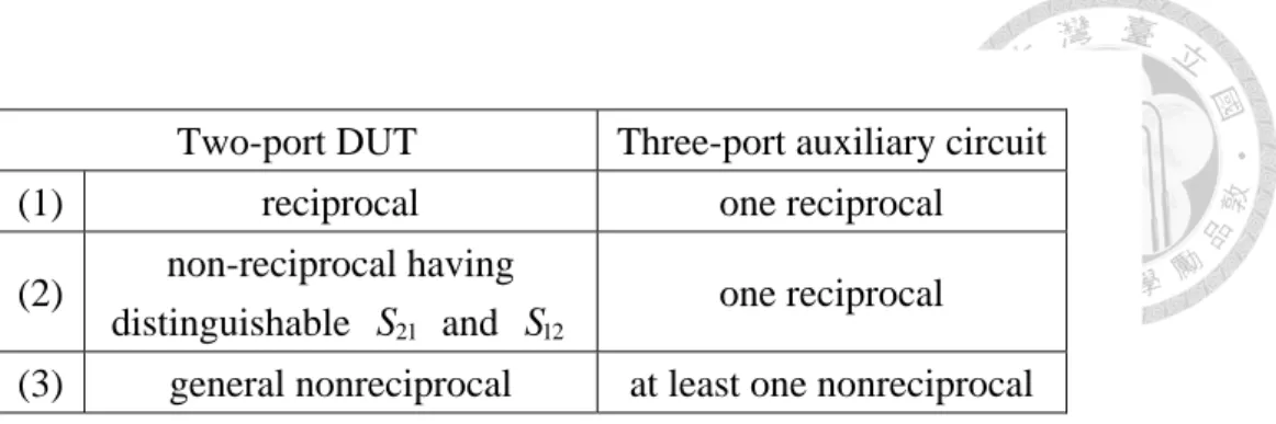
This leads that one should use a reciprocal auxiliary circuit and (2.12) to solve the

transmission coefficient of a reciprocal DUT as suggested in row (1) of Table 3.1.

Further discussion on using a reciprocal auxiliary circuit for a two-port reciprocal DUT

will be given in the Section 3.3 based on the accuracy consideration.

For certain two-port nonreciprocal DUTs whose S12 and S21 are distinguishable,

with the use of one reciprocal auxiliary circuit as suggested in row (2) of Table 3.1, one

could easily identify S21 and S12 from the roots of (2.11). The other additional

auxiliary circuit as described in Section 2.1.2 to identify the correct S21 is therefore not

necessary. The resulting number of one-port measurements is then four.

28

Amplifier is a typical example to use only one reciprocal auxiliary circuit. The

larger root of (2.11) should be S21 representing the amplifier forward gain, while the

other is S12. Isolator is another typical example, because its |S21| >> |S12|.

As for a general two-port nonreciprocal DUT, one needs two three-port auxiliary

circuits. Note one of the auxiliary circuits should be nonreciprocal as suggested in row

(3) of Table 3.1. Otherwise, the two sets of roots will be identical. Table 3.1 summarizes

the suggestion on selecting the proper auxiliary circuit for a two-port DUT.

3.2 Two-port active network

This section will discuss the solvability of (2.18) for a two-port active DUT in

terms of the auxiliary circuit. As described in Section 2.2, one can reconstruct the

S-matrix of a two-port active DUT with five one-port measurements and (2.18).

Specifically, the S-matrix is determined through the following matrix equation

=

ΣX B

where

(1) (1) (1) (1) (1) (1) (1) (1) (1) (1)

1 1 2 2

(2) (2) (2) (2) (2) (2) (2) (2) (2) (2)

1 1 2 2

(5) (5) (5) (5) (5) (5) (5) (5) (5) (5)

1 1 2 2

... ... ... ... ...

a a b b c c

a a b b c c

a a b b c c

N BD N BD N BD N BD N BD

N BD N BD N BD N BD N BD

N BD N BD N BD N BD N BD

 − − − − −

 − − − − −

− − − − −

 Σ=



 

 

 

 

and

29

X

11

22

12

21

det

S S S S S

 

 

 

 

= 

 

 

 

(1)

(2)

(3)

(4)

(5)

B B B B B

 

 

 

 

= 

 

 

 

.

Note that the superscripts in (3.5) and (3.6) denote the five one-port measurements. The

other superscripts used in the expressions in Chapter 2 denote the terminated port of

DUT and the corresponding termination.

By substituting (2.8) and (2.9) into (2.18), the coefficients of S12 and S21 can be

represented as

1 1 12 31 32

N −BD =a a +Ba (3.7)

2 2 21 13 23

N −BD =a a +Ba . (3.8)

From (3.7) and (3.8), one can find that if a reciprocal auxiliary circuit is used, the

coefficients of S12 and S21 are identical. Therefore, if the five auxiliary circuits used

in Section 2.2 are all reciprocal, the third and fourth columns of

Σ

As the result, the determinant of

Σ

that at least one of the five auxiliary circuits used in Section 2.2 must be nonreciprocal

to guarantee the solvability of (3.5). It is also consistent with the suggestion given in

Table 3.1.

3.3 Two-port reciprocal network

This section will discuss the selection of the auxiliary circuit to improve the