Hung-Lung Lee
Shyang-Jye Chang
Sheng-Jye Hwang
Associate Professor, e-mail address: [email protected]Department of Mechanical Engineering, National Cheng Kung University, Tainan, Taiwan
Francis Su
S. K. Chen
ChipMOS Technologies Inc., Tainan, TaiwanComputer-Aided Design of a TSOP
II LOC Package Using Taguchi’s
Parameter Design Method to
Optimize Mold-Flow Balance
This paper presents a methodology for TSOP II LOC packaging design. The design objectives are: 1) to optimize mold-flow balance, which in turn minimizes air traps, and 2) to minimize manufacturing variability, which implies optimal quality. A mold-flow simu-lation tool called C-MOLD is used to evaluate various design configurations. Taguchi’s robust design method is used for manufacturing variability considerations. The simulated results are verified with experimental flow patterns produced by means of ‘‘short shots.’’ In the nomenclature of the Taguchi method, mold-flow balance was chosen as quality characteristics and select a set of design parameters called control factors. The objectives are to find the levels of the control factors, which optimize the flow balance, and, at the same time, minimize the sensitivity of the variations of the control factors.
关DOI: 10.1115/1.1569957兴
Keywords: TSOP II LOC Package, Taguchi Method, Mold-Flow Balance
Introduction
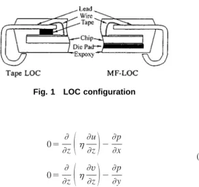
In LOC共lead on chip兲 packaging, inner leads of the leadframe are arranged right above the chip rather than surrounding the chip. The process of LOC packaging is similar to traditional SOJ or TSOP packaging. Schematic of LOC configuration is shown in Fig. 1. There are two types of LOC configurations: tape-LOC and MF-LOC. MF-LOC共multiframe LOC兲 packaging uses two pieces of leadframes while tape-LOC packaging uses polyimide tape to connect chip and leadframe. Because of shortened wire span and reinforced die support, the wire sweep and paddle shift problems are no longer the major concerns for LOC packaging. Instead, the air-trap problem is one of the most concerned problems in the design stage of a new LOC package.
The major factors that affect mold-flow patterns of EMC 共ep-oxy molding compound兲 are dimensions of die and location of mold cavity. The flow pattern of molding compound is extremely sensitive to the geometry of mold cavity. Especially, when the melt front advancement encounters a large thickness variance of flow path or unbalanced thickness distribution between upper and lower subcavities, the short shot or air traps will easily occur during molding process. Another important factor that affects the molding performance is the leadframe layout design. The lead-frame functions not only as signal connector between die and PCB but also as die support and helps producing turbulent flow to reduce the possibility of air traps during molding process. To com-promise the limited space in mold cavity and inherited structure of TSOP LOC-type package, the upper subcavity is relatively smaller than the lower sub-cavity. The cross-flow flowing through leadframe openings from lower to upper subcavities is the primary way that melt flow runs into upper sub-cavity. No doubt the lead-frame layout is a significant factor in IC packaging design.
The object of this study is to use the software of CAE 共Com-puter Aided Engineering兲, C-MOLD, to simulate the mold flow stage of microchip encapsulation. The experimental and simulated results are compared and they are satisfactorily matched. At the
same time, the Taguchi method was used to reduce performance variance during manufacturing. The procedure makes design process more effective and systematic.
Analysis
CAE software was used to simulate molding process of IC packaging in this study. The advantage of using CAE software is to find out optimal levels of control factors by engineers before the IC product is produced. C-MOLD is a commercially available software which uses finite element method to simulate polymer forming process. The input data include three major sections: fi-nite element mesh, material properties, process parameters.
Governing Equations. EMC is a thermosetting material and C-MOLD’s Reactive Molding packaging is chosen for the simu-lation. This package can predict flow situation of thermosetting material like flow pattern, air traps location, clamp force, etc., during IC molding process. The elasticity of the epoxy molding compound is considered negligible if the degree of cure of the sample is low. During filling stage of encapsulation, the degree of cure of the sample is low. Elasticity of the fluid is negligible and thus assume the flow to be a generalized Newtonian fluid. Also, since the thickness of the chip cavity is typically much smaller than its width, the generalized Hele-Shaw approximation can be used关1兴. Using these approximations, one can obtain the govern-ing equations: continuity equation, momentum equations, energy equation, kinetics equation, constitutive equation for the flow analysis关2兴.
Continuity Equation. Including the possible compressibility of the melt, the continuity equation can be written as follows:
t ⫹ 共u兲 x ⫹ 共v兲 y ⫹ 共w兲 z ⫽0 (1)
where u,v, and w are respectively the velocities of the x, y and z components, and is the density. Here, x, y are the in-plane di-rection, and the z direction is perpendicular to the plane direction. Momentum Equations. Neglecting the inertia terms and us-ing the thin cavity approximation, the momentum equations in the x and y directions can be written as follows:
Contributed by the Electronic and Photonic Packaging Division for publication in the JOURNAL OFELECTRONICPACKAGING. Manuscript received by the EPPD Di-vision December 16, 2001. Associate Editor: G. De Mey.
0⫽ z
冉
u z冊
⫺ p x (2) 0⫽ z冉
v z冊
⫺ p ywhererepresents viscosity. The momentum equations in z direc-tion can simply result in constant pressure in z direcdirec-tion.
Energy Equation. By assuming a thin cavity and including heating due to shearing and curing, the energy equation can be written as follows: Cp
冉
Tt ⫹uT x ⫹v T y冊
⫽ z冉
K T z冊
⫹␥˙⫹ d␣ dt⌬H (3) where Cpis the heat capacity, K is the thermal conductivity,␥˙ is the shear rate,␣ is the conversion, and ⌬H is the reaction heat.Kinetics Equation. This equation involves the degree of cure with time. In this study, the empirical equations of Kamal关2兴 are used ␣⫽兰0 t⌬Hdt 兰0⬁⌬Hdt d␣ dt⫽共k1⫹k2␣ m1兲共1⫺␣兲m2 (4) k1⫽a1exp共⫺E1/T兲
k2⫽a2exp共⫺E2/T兲
where␣ is the EMC conversion, and the k1, k2, a1, a2, m1, m2,
E1, E2, are all fitted constants in the Kamal equations.
Constitutive Equation. In order to account for the effect of the thermosetting reaction on the viscosity, the modified Cross equation关2兴 was used to describe the rheological properties
共␣,T,␥˙兲⫽ 0共T兲 1⫹
冉
0共T兲␥˙ *冊
1⫺n冉
␣g ␣g⫺␣冊
共C1⫹C2␣兲 (5) 0共T兲⫽B exp共Tb/T兲where␣, ␣g, C1, C2and B are the resin conversion, the conver-sion at gelation, two fitted constants and an exponential-fitted pa-rameter, respectively.
Cross-Flow Analysis. For traditional microchip encapsula-tion modeling method in C-MOLD, ‘‘part runners’’ and ‘‘connec-tors’’ are often used to model the openings of leadframe关3兴. How-ever, part runners and connectors are only one dimension in geometry; they cannot figure out air traps in the early design stage, in IC packaging. Therefore, in order to simulate the flow resistance of the leadframe opening, a two-dimensional approach was used: the cross-flow element. The Hele-Shaw approximation is still used for cross-flow analysis in this modeling methodology. The leadframe openings that cross-flow flow through are modeled as ‘‘regions’’ in C-MOLD关4兴.
In modeling the openings in flow analysis using Hele-Shaw approximation, the juncture loss associated with the flow across the openings needs to be considered. Because of the juncture loss, we cannot use the same size openings in the model. Equations共6兲 to 共9兲 help calculating the thickness of the openings when the juncture loss is considered.
b1*⫽A⫺共1/共2n⫹1兲兲 (6) where A⫽
冉
2n 1⫹2n冊
n1 L再
2冉
2n⫹1 2n冊
n 1 n冉
sin 冊
2n冉
1 b0 2n⫺ 1 b1 2n冊
⫹1n冉
sin 2 冊
n冉
1 b0 2n⫺ 1 b1 2n冊
⫹ 8 b1 2n冕
0sin2n⫺1共 cos ⫺sin 兲
n⫹1 d⫹
冉
1⫹2n 2n冊
n L b1 2n⫹1 ⫹2冉
1⫹2n2n冊
n Kx b1 2n冎
(7) and Kx⫽再
0 Z⬍0.01 A⫹B ln共Z兲 when 0.01⬍Z⬍0.33 C Z⬎0.33 (8)where Z is L/b1. In the above equations, n is the power-law index, b1is half of the actual opening width, and b0is half of the distance between the solid region, as shown in Fig. 2.
In Fig. 2, the solid region represents the leadframe region and b1*is half of the opening width to be used in the modeling. The length of the opening in the model will be the thickness of the leadframe. When n⫽0.74, the values of A, B, and C are 1.2041, 0.2501, and 0.903 respectively. The values of A, B, and C only slightly depend on n, so these values can be used for other values of n. As an approximation, can be taken as /2. The integral term in Eq.共7兲 can be approximated by
冕
0sin2n⫺1共 cos ⫺sin 兲
n⫹1 d⬵0.4504⫺0.2042n ⫹0.04324n2
(9) If the foregoing equations are too complicated, as a rule of thumb, use 1/3 of the actual opening width in the leadframe as the width in the model.
Fig. 1 LOC configuration
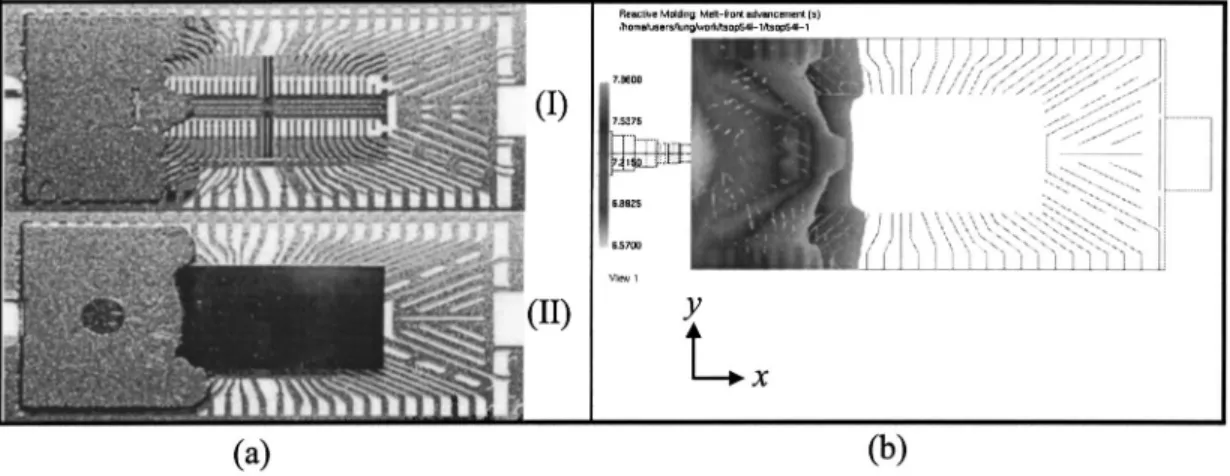
Fig. 3 Comparisons of experimental short shot and simulation results at 1Õ3 shot„a…experiment„I…top view
„II…bottom view,„b…simulation
Fig. 4 Comparisons of experimental short shot and simulation results at 2Õ3 shot„a…experiment„I…top view
„II…bottom view,„b…simulation
Fig. 5 Comparisons of experimental short shot and simulation results at 9Õ10 shot„a…experiment„I…top view
TSOP II LOC Packaging Simulation Experiment The study case of this experiment is TSOP II 54L LOC pack-age. The chip cavity size is 22.22 mm共length兲⫻10.16 mm 共width兲 ⫻1.00 mm 共thickness兲. The epoxy molding compound used for the experiment is HITACHI CEL-9200-XU. The mold wall tem-perature was 175°C and the transfer time was 10.2 s. Short Shot was made to evaluate the flow pattern. By comparing the experi-mental and simulated results, Figs. 3–5 show that the simulated flow pattern can match the experimental results at 1/3, 2/3, and 9/10 shots 关3兴 very well. Air traps location is shown in Fig. 6. These figures show that the modeling method can predict flow pattern of TSOP II 54L LOC precisely, and hence the simulation is reliable.
Taguchi Method
Robust product design offers a reliable, quantifiable, and effi-cient means to attain the best quality in all stages of product commercialization. By defining on-target performance and vari-ability, robust design methods provide engineers the means to make products and processes insensitive to sources of variability. Robust design helps us quantify the cost of quality. From an en-gineering point of view, it provides us for measuring where we are, where we want to be, and how to get there.
Taguchi’s method has been used to improve quality of products for a long time. It uses the lowest cost to obtain the best quality by tools such as S/N ratio and orthogonal arrays. By this way, the product quality is insensitive to variance caused by ‘‘noise fac-tors’’ and an optimal parameter combination can be obtained.
TSOP Experiment. In this study, ‘‘flow balance’’ is chosen to be the quality characteristics. ‘‘Flow balance’’ means the same location and configurations of melt front advancement between upper and lower subcavities. When melt front advancement of lower subcavity reaches the end of the mold, it will in turn flow upward and meet melt front advancement of upper subcavity to form air traps. Air traps will not only affect the appearance of the IC product, but also reduce its reliability. Further, difference of melt front locations will cause pressure difference, and in turn induce the paddle shift and wire sweep. During molding process, the smaller melt front area difference represents the better flow balance. Since we cannot measure all relative mold-flow area dif-ference, we choose only 1/3, 2/3, and 9/10 short shots which represent a large thickness variance of flow path to measure the melt front area difference between upper and lower subcavities.
By a brainstorming in early design stage, all possible design parameters that affect the performance in the IC packaging pro-cess were considered. The most important eight control factors and their levels for the experiment are shown in Table 1.
The Noise Factors Experiment. In order to carry out the experiment effectively, we chose to run a noise experiment before the main experiment. The primary goal of the noise experiment is to identify the few noise factors and their settings that cause most of the variability in the system being optimized. This goal for the
Fig. 6 TSOP LOC air traps location
Table 1 Control factors and levels table
FactorsLevels Level 1 Level 2 Level 3
共A兲Dummy cavity *YES NO 共B兲Leadframe design Front deflector cut *Original Back deflector cut 共C兲Chip thickness
11.5 mil *12.5 mil 13.5 mil
共D兲Leadframe with down-set *Original 50m 100m 共E兲filling time 9.2 s *10.2 s 11.2 s 共F兲Inlet melt temperature 75°C *80°C 85°C 共G兲Mold temperature 170°C *175°C 180°C
共H兲EMC Nitto Denko
MP-190M *Hitachi 9200-XU SHINETSU CHEMICAL KMC-188-1 *indicate original process parameters
Table 2 Noise factors and levels table
FactorsLevels Level 1 Level 2
共a兲EMC density ⫺5% ⫹5%
共b兲Chip thickness ⫺4% ⫹4%
共c兲Leadframe with
down-set ⫺5% ⫹5%
共d兲filling time ⫺4% ⫹4%
共e兲Inlet melt temperature ⫺3% ⫹3%
共f兲Mold temperature ⫺3% ⫹3%
Table 3 L12 table experiment and results„mm2…
Run a B C D e f 1/3 short shot 2/3 short shot 9/10 short shot
1 1 1 1 1 1 1 15.690 20.499 20.950 2 1 2 2 2 2 2 15.103 21.244 22.237 3 1 1 1 2 2 2 15.442 20.115 20.882 4 1 2 2 1 1 2 14.832 21.131 21.921 5 1 1 2 1 2 1 14.922 19.912 20.724 6 1 2 1 2 1 1 14.810 20.205 20.837 7 2 2 2 1 2 1 14.584 21.018 21.672 8 2 2 1 1 1 2 14.493 20.815 21.447 9 2 1 2 2 1 1 15.035 19.912 20.657 10 2 1 2 2 1 2 15.035 20.002 20.747 11 2 1 1 1 2 2 15.351 19.731 20.205 12 2 2 1 2 2 1 14.561 20.589 21.334
noise factor experiment is accomplished by decomposing the data from the noise factor runs using analysis of means共ANOM兲 to analyze the magnitude and directionality of the noise factor ef-fects. Other goals for the noise experiment include: benchmarking performance, perfecting the experimental procedure, and testing the magnitude of measurement error.
The selection of noise factors is critical to the robustness. It is important to know what the causes of variability are, because these are the sources of customer dissatisfaction. Noise factors are defined as factors that can influence the performance of a system and are not under our control共either impossible or expensive to control兲 during the intended use of the product. Noise factors can be external to the design. Generally, these are controlled by cus-tomers. Noise factors can also be internal to the design. These are design parameters whose nominal level may be specified, but manufacturing variation and deterioration result in deviation from the intended target. Because our experiment is the form of the numerical simulation, it is almost impossible to simulate the ex-ternal noise, i.e., variability from outside of the product or pro-cess. For the product design purpose, we choose unit-to-unit variation, i.e., variability due to manufacturing processes, as our noise factors. Six process parameters was chosen as noise factors and their manufacturing variation deviation set to be experiment levels. Noise factors and levels of noise experiment are shown in Table 2.
The significant noise factors are combined and used in the pa-rameter optimization experiment to test the robustness of the con-trol factor combinations. The goal is to compound the noises for the parameter optimization experiment into two groups using the directionality of the noise factor effects. Those noise factor levels that cause an increase in the response are grouped together into CNF⫹, and those noise factor levels that cause a reduction in the response are grouped together into CNF⫺. After noise experi-ment, we decide CNF⫹⫽a1b2c2, CNF⫺⫽a2b1c1. The noise
ex-periment using an L12 array is shown as Table 3. Table 4 shows 9/10 short shot melt front area difference data and use the data to figure out Fig. 7. Table 5 shows a comparison of predictive re-sponse and the confirmation of noise experiment. Figure 8 shows how to measure 9/10 short shot melt front area difference by using image processing software.
These two groups, CNF⫹and CNF⫺, are used for each com-bination of the control factor. For an L18 array, this results in a total of 36 runs for the parameter optimization. The parameter optimization experiment can now be run using an L18 array and the two compound noise factors, N1 and N2, represent CNF⫹, which is shown as Table 6, and CNF⫺, respectively.
Results
In this study, we seek to minimize melt front area difference to attain the flow balance. The smaller-the-better S/N ratio is based on the small-the-better loss function. The derivation of the smaller-the-better type S/N ratio is based on the following ideas: 1兲 quality characteristics or response values are continuous and nonnegative, 2兲 the desired value of the response is zero, and 3兲 the goal is simply to minimize the mean and variance simulta-neously. The smaller-the-better S/N ratio is defined by Eq.共10兲.
S/NSTB⫽⫺10 log
冉
1 n兺
i⫽1 n yi2冊
⫽⫺10 log共S2⫹y¯2兲 ⫽⫺10 log共MSD兲 (10)After the main parameter experiments, we know the optimal assembly of control factors and levels of 1/3 shot, 2/3 shot, 9/10 shot are B3H2C2G2, D1C1H1B3, B3C2D2H2, respectively, by
Fig. 7 9Õ10 short shot factor effects plot for the noise array„mm2… Table 4 9Õ10 short shot response table„area…
Response table 9/10 short shot melt from area difference共mm2兲
Level A b c D e F
1 21.259 20.694 20.943 21.153 21.093 21.029
2 21.010 21.575 21.326 21.116 21.176 21.240
⌬ 0.248 0.880 0.384 0.038 0.083 0.211
Ranking 3 1 2 6 5 4
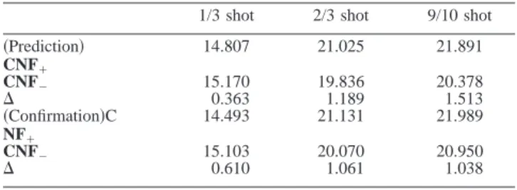
Table 5 Comparisons of predictive response results and con-firmation experiments
1/3 shot 2/3 shot 9/10 shot
共Prediction兲 CNF⫹ 14.807 21.025 21.891 CNF⫺ 15.170 19.836 20.378 ⌬ 0.363 1.189 1.513 共Confirmation兲C NF⫹ 14.493 21.131 21.989 CNF⫺ 15.103 20.070 20.950 ⌬ 0.610 1.061 1.038
S/N ratio response table. In the molding process, the optimal as-sembly of control factors and levels are not always the same in all cases. However, from the underlying study, we may conclude that the major factors affecting molding flow process are leadframe design, geometrical dimensions of die and space allocation of mold cavity. The process parameters may not affect quality char-acteristics very much.
For considering all mold flow process, we also treat short shot location as the ‘‘surrogate’’ noise共a noise due to measuring time, location, etc.兲. We conduct the main experiment again by eight control factors and the two compound noise factors and the sur-rogate noise in L18 array. Table 7 shows the experiment results. By S/N ratio shown in Table 8 and Fig. 9, we know the leadframe cut back deflector is the main factor that affects quality character-istic. The optimal assembly of control factors and levels of all design is B3D2C2H2. After analysis and prediction of the opti-mum performance, we improve the S/N ratio by 2.374 db. This means we improve 23.9% variance of flow balance for TSOP II
Fig. 8 Measure 9Õ10 short shot melt front area difference Table 6 L18 array experiments
NO A B C D E F G H N1 N2 Mean S/N 1 1 1 1 1 1 1 1 1 2 1 1 2 2 2 2 2 2 3 1 1 3 3 3 3 3 3 4 1 2 1 1 2 2 3 3 5 1 2 2 2 3 3 1 1 6 1 2 3 3 1 1 2 2 7 1 3 1 2 1 3 2 3 8 1 3 2 3 2 1 3 1 9 1 3 3 1 3 2 1 2 10 2 1 1 3 3 2 2 1 11 2 1 2 1 1 3 3 2 12 2 1 3 2 2 1 1 3 13 2 2 1 2 3 1 3 2 14 2 2 2 3 1 2 1 3 15 2 2 3 1 2 3 2 1 16 2 3 1 3 2 3 1 2 17 2 3 2 1 3 1 2 3 18 2 3 3 2 1 2 3 1
Table 7 Experiment results„mm2…
NO N1 N2 Mean S/N 1/3 2/3 9/10 1/3 2/3 9/10 1 15.329 18.963 20.499 16.254 19.054 20.566 18.444 ⫺25.368 2 13.794 21.966 19.483 13.997 19.189 18.557 17.831 ⫺25.143 3 15.148 24.224 23.050 14.584 23.953 24.675 20.939 ⫺26.600 4 16.661 19.370 20.882 17.496 21.198 22.237 19.641 ⫺25.908 5 13.907 19.392 20.273 15.645 18.060 20.205 17.914 ⫺25.140 6 12.055 28.152 24.675 13.613 23.727 22.937 20.860 ⫺26.723 7 15.690 18.918 7.337 16.932 18.015 7.134 14.004 ⫺23.424 8 12.913 22.779 7.405 14.313 19.279 7.021 13.952 ⫺23.574 9 14.561 19.641 7.314 15.509 19.234 7.066 13.888 ⫺23.397 10 14.968 22.982 20.115 14.516 20.657 19.708 18.824 ⫺25.608 11 14.606 19.754 19.573 14.742 19.934 19.663 18.045 ⫺25.203 12 14.313 23.140 21.447 15.126 20.769 20.589 19.231 ⫺25.806 13 13.929 20.295 20.724 15.577 19.099 20.611 18.373 ⫺25.373 14 13.794 24.449 20.679 15.035 21.605 20.634 19.366 ⫺25.900 15 16.300 19.754 21.063 17.338 19.370 21.356 19.197 ⫺25.704 16 13.703 23.253 7.947 13.816 20.995 7.518 14.539 ⫺23.921 17 16.841 19.731 8.308 18.106 20.137 8.195 15.220 ⫺24.101 18 13.703 21.334 8.308 15.780 19.799 8.195 14.520 ⫺23.742
Table 8 SÕNratio response table
Response table S/N ratio共db兲
Level A B C D E F G H 1 ⫺25.031 ⫺25.621 ⫺24.934 ⫺24.947 ⫺25.060 ⫺25.157 ⫺24.922 ⫺24.960 2 ⫺25.040 ⫺25.791 ⫺24.843 ⫺24.771 ⫺25.009 ⫺24.950 ⫺25.117 ⫺24.856 3 ⫺23.693 ⫺25.329 ⫺25.388 ⫺25.037 ⫺24.999 ⫺25.067 ⫺25.290 ⌬ 0.009 2.098 0.485 0.616 0.050 0.208 0.195 0.434 ranking 8 1 3 2 7 5 6 4
Fig. 9 Factor effectsSÕNratio table
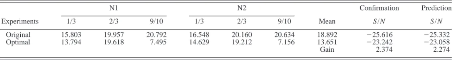
Fig. 10 Confirmation experimental model and melt front advancements Table 9 Confirmation experiment table
Experiments N1 N2 Confirmation Prediction 1/3 2/3 9/10 1/3 2/3 9/10 Mean S/N S/N Original 15.803 19.957 20.792 16.548 20.160 20.634 18.892 ⫺25.616 ⫺25.332 Optimal 13.794 19.618 7.495 14.629 19.212 7.156 13.651 ⫺23.242 ⫺23.058 Gain 2.374 2.274
Table 10 ANOVA table
Factor SS Dof Pooled Var F P %
A 0.00036 1 Y B 16.302 2 8.1510 269.0102 0.000% 84.91% C 0.7992 2 0.3996 13.1890 0.211% 4.16% D 1.2097 2 0.6049 19.9625 0.049% 6.30% E 0.0076 2 Y F 0.1414 2 Y G 0.1233 2 Y H 0.6161 2 0.3080 10.1659 0.491% 3.21% Error 0.2727 9 0.0303 1.42% Sm 11281.52 1 100% St 11301.42 18
LOC mold-flow analysis. Table 9 shows the confirmation experi-ment table. Figure 10 shows the confirmation experiexperi-ment model and the melt front advancements.
ANOVA共analysis of variance兲 is a statistic technique that en-ables the engineers to quantitatively estimate the relative contri-bution of each control factor to the overall variation and expresses it as a percentage. ANOVA uses a mathematical technique known as the sum of squares to quantitatively examine the deviation of the control factor effect response averages from the overall experi-mental mean response. Form ANOVA table共Table 10兲, we know the control factor B共leadframe design兲 is the major factor which contributes 84.9% of the response. The factors D共leadframe with down-set兲, C 共chip thickness兲, H 共EMC兲 and A 共Dummy cavity兲, E 共filling time兲, F 共Inlet melt temperature兲, G 共mold temperature兲 are attributed to random experimental errors.
Conclusion
The accomplishment of this study is to improve the numerical simulation method to reproduce the mold flow stage of microchip encapsulation by C-MOLD. We use the two-dimensional simula-tive technique, cross-flow element, to simulate the flow resistance of the leadframe opening. By comparing the experimental and simulated results, we obtain a good match between simulated flow pattern and the experimental results. The simulation technique is reliable.
Taguchi’s method was used to reduce variability for the robust design of mold-flow simulation of IC packaging. The object is to
find out the optimal combination of control factors and levels. Using this methodology, the design procedure is more effective and systematic. By Taguchi method, we can know clearly what factors affect the flow balance for TSOP II LOC 54L 64M DRAM mold flow analysis. The major factors that affect molding flow process are geometrical dimensions of chip and space allocation of mold cavity and leadframe design; the material property is the next important factor. The optimal assembly of control factors and levels improve 23.9% variance of flow balance.
Acknowledgment
This work was financially supported by ChipMOS Company in Tainan, Taiwan.
References
关1兴 Nguyen, L. T., Danker, A., Santhiran, N., and Shervin, C. R., 1992, ‘‘Flow
Modeling of Wires Sweep during Molding of Integrated Circuits,’’ ASME Winter Annual Meeting, 11/8-13 Anaheim, CA, 1.
关2兴 Han, S., and Wang, K. K., 1995, ‘‘Flow Analysis in a Cavity with Leadframe
during Semiconductor Chip Encapsulation,’’ Advanced in Electronic
Packag-ing, ASME EEP-Vol. 10–1.
关3兴 Su, Franci, Lu, Richard, and Fan, James, 1998, ‘‘The Application of
Cross-Flow Modeling Techniques for TSOP II 54L Loc Package,’’ C-MOLD
Micro-chip Encapsulation Users’ Conference.
关4兴 ‘‘C-MOLD Microchip Encapsulation User’s Guide,’’ 1997, Advanced CAE