DETERMINATION OF OBJECT POINT COORDINATES BY
MMS IMAGE SEQUENCES USING MULTIPLE IMAGE
MATCHING
Cheng-Kai Wang, Chia-Yu Hsieh, Yi-Hsing Tseng
Department of Geomatics, National Cheng-Kung University. No,1, University Road, Tainan 701, Taiwan [email protected], [email protected], [email protected]
ABSTRACT: The coordinates of interested points can be determined by space intersection of the images, whose
interior and exterior orientation parameters are determined from the navigation and calibration data. Obtaining conjugate points of image sequences by image matching is much more efficient than manual measurement. However the factors of scale variations, different field of view, and occlusion may result in incorrect matching points. In this research, image matching in object space with virtual surface is proposed to overcome the problem of matching in image space. The process to filter out occluded images is proposed, and the remaining useful images are kept for multiple image matching with multiple windows, which is developed to ease the problems caused by complex backgrounds. The test results of the experiments show the proposed method can deliver correct matching results good to about 90%. The determined coordinates are about 10 cm in precision, and about 50 cm in accuracy. Accuracy can be improved, if the positioning and orientation system of the MMS can be improved.
KEY WORDS: MMS image sequences, multi-image matching, object space, multi-window matching
1. INTRODUCTION
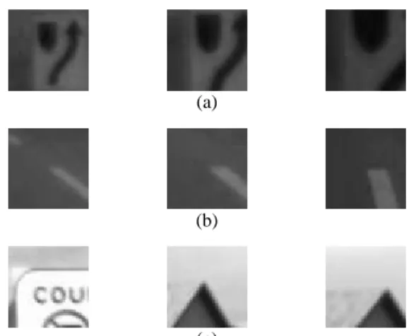
Mobile Mapping System (MMS) mounted on a measurement vehicle integrates the camera system and positioning system to acquire the images and positioning data regularly and simultaneously. In the earlier years, the data is captured by analogy cameras such as Alberta MHIS (Lapucha 1990) and GPSVan(El-Sheimy 1996). Followed the development of GPS and INS/IMU, the direct geo-referencing system is launched with multi-cameras to obtain the image sequences so far. For example, the VISAT II developed by the University of Calgary. The coordinates of interested points can be calculated through space forward intersection of the overlap images. For such image sequences with high-ratio overlaps, image matching is more efficiently to obtain the conjugate points than manual measurement. The matching methods can be divided into the three categories which are area-based, feature-based and relational matching. The most common methods are area-based and area-based methods. Comparing to feature-based matching, the area-feature-based matching which utilizes the variation of gray values is more reliable without losing the feature information(McGlone 2004). For this reason, our research is based on the area-based matching. However the area-based matching is suffered from the three factors: scale variation, different field of view, and occlusion (see Figure 1). In this paper, image matching in object space with virtual surface is presented to overcome these problems.
2. MULTIPLE IMAGE MATCHIN IN OBJECT SPACE
(a)
(b)
(c)
Figure 1. Problems in matching. (a)scale variation, (b)different field of view, occlusion
2.1 Matching in Object Space
In theory, if a plane in object space is back projected in image sequences which all capture this plane without occlusion, the projected planes derived from these overlap images will form an identical projected image. Thus if an assuming surface in object space is projected in the overlap images and these projected surfaces lead to high correlations which means they are similar to each other, the assuming surface is then considered to match the real surface. In this way, the matching method is called matching in object space.
The difference between matching in object space and image space is that matching in object space is less suffered from the imaging geometry. With matching in object space, several surfaces need to be assumed and the orientations of these assumed surfaces have to be close to
the orientations of the real surfaces so that the two problems, scale variations and different field of view, can be solved. The most common matching method in object space is Vertical Line Locus (VLL) which sets a series of assuming planes along a vertical direction through a fixed planar location in object space. These assuming planes are then back projected to the images to acquire the pixel values and form the plane images. These plane images are therefore used for matching. VLL is firstly proposed for DTM generation. In this paper, the matching idea is based on VLL with a little modification. The assuming planes are generated along the ray begins from perspective center to the interested point. Figure 2 shows the conception of matching in MMS image sequences.
Ln
L ~1 denotes the assuming planes in object space.
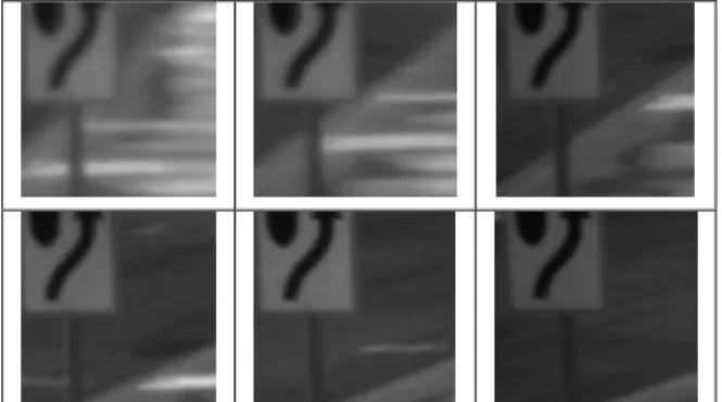
Figure 2. Conception of matching in MMS images Each assuming plane can be considered as a plane image and the pixel values of this plane can be filled with the values of the MMS images by back projection. Figure 3 shows an example of 6 back projected results from an assuming plane. The results indicate that the scale variation is reduced by VLL.
Figure 3. Results of back projection of assuming planes On the other hand, adjusting the assuming plane closer to real location can solve the problem of different field of view (see Figure 4 and Figure 1(b)).
2.2 Matching Indicators
Once the interested point is chosen, a series of assuming planes are created. Each plane can generate several projected images and these projected images are used to match to each other. The matching indicator used in this paper is called Yet Another Reconstruction Dataprogram (YARD) which is proposed by (Wiman 1998). 2 2 ( )( ) ( ) ( ) ijk k ijk k i j k ijk k ijk k i j k i j k g g f f g g f f
(1) ; 1 ijk l ijk g f l k n
In Wiman’s (1998) study, there is no primary image while we do have in our research. Thus the YARD is modified as equation (2) for our application.
2 2 ( )( ) ' ( ) ( ) ij ij i j ij ij i j i j g g f f g g f f
(2)where gij denotes the primary image and fij denotes the average of projected images.
Each assuming plane will derive a value which evaluates the matching similarity. The maximum indicates that the corresponding assuming plane is the best fitting to the real plane.
2.3 Window Selection
To avoid the influence of background of the target on the matching results, this paper adopts the idea which is called CLR (Center, Left, Right) method with a slight modification. This method treats the interested point not only on the ceter of a window but also on the top, bottom, left, right side and so on (Figure 4). Therefore, each assuming plane will contain 9 sub-windows and each sub-window will derive a matching indicator which is calculated by the projected images.
3. MATCHING STRATEGY
3.1 Location Estimation of Assuming Plane
The location of assuming plane needs to be estimated approximately. Two methods are used for estimation. The first is to measure the conjugate point manually and one can obtain the 3D coordinates of the interested point by forward intersection. The second is to search the approximated location in object space directly. A distance along the ray (from perspective center to the interested point) from the primary image to the farthest point is set to 200 meter. Then the assuming planes are generated along the distance in every 5 meter. Using these assuming planes, one can calculate all the YARD values and the best matching of assuming plane will be selected as the initial location. Then a searching distance 20 meter along the ray whose center is on the initial assuming plane is set. Again the assuming planes are generated between the searching distance in every 1 meter. The best matching assuming plane will be selected as the final initial assuming plane.
3.2 Conjugate Image Filtering
After obtaining the initial assuming plane, the plane will be back projected to the primary image and the images before and after the primary image to obtain the projected images. The projected images are therefore used for calculating the values sequentially. If a projected image is added and the value decreases more than 0.1, the projected image will be removed. The remaining projected images will be retained for multi-window matching.
3.3 Mutli-Window Matching
As mentioned in section 2.3, each projected image is separated into 9 sub-images (sub-windows). The corresponding sub-images from conjugate images are used for matching. As section 3.1, a shorter searching distance through the initial location is set as 3 meters. The interval between assuming planes are 10 centimetres. With 9 sub-images, each assuming plane will produce 9
values. An example is shows as Figure 5. One can see that the 9 curves can be separated into two groups. One group contains 5 curves which appear high values and the other contains 3 curves appear low values. It is easily to exclude the three cures by an interval threshold. If the interval between two curves is larger than 0.1, the lower curve will be discarded. The remaining curves denote the best matching sub-windows of this target and each curve corresponding to its sub-window will generate the matching location using the maximum of each curve. A more accuracy location will be the average of these matching locations from the remaining sub-windows.
4. EXPERIMENT RESULTS AND ANALYSIS
Figure 5. Matching using multi-windows
4.1 The VISAT Test Data
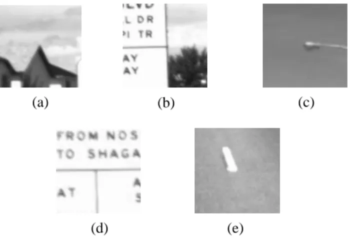
The VISAT Test Data is provided by Department of Geomatics Engineering, University of Calgary. In this research, the point features in the images are divided into 5 categories. Figure 6 shows the 5 types of point features.
Figure 6. The point feature in the street view. (a)point feature is clear with pure background, (b)point feature is
clear with complex background, (c)point feature is unclear with pure background, (d)point feature is clear with no background, (e) point feature is suffered from the
different field of view.
We chose 10 points of each type. Among the 50 test points, 38 points were matched successfully while 12 points failed. The correct matching ratio is about 80%. With the 12 failed cases, the conjugate points are re-selected by manual measurements, 11 feature points were matched correctly only one still failed. The Matching ratio improves to 98%.
4.2 The NCKU Test Data
The second test data is generated from the MMS vehicle developed by Department of Geomatics, National Cheng-Kung University. A test field with several high-accuracy control points is established in a block campus. However a system error is still contained in the positioning system which results in a discrepancy. The discrepancy can be observed if the control point is back projected to the image (see Figure 8).
Window1 Window2 Window3 Window4 Window5 Window6 Window7 Window8 Window9 59 58 57 56 55 54 53 52 51 50 49 48 47 46 45 44 43 42 41 40 39 38 37 36 35 34 33 32 31 30 29 28 27 26 25 24 23 22 21 20 19 18 17 16 15 14 13 12 11 10 9 8 7 6 5 4 3 2 1 0 1 0.8 0.6 0.4 0.2 0 -0.2 -0.4 -0.6 -0.8 -1 Spatial index Y A R D (a) (b) (c) (d) (e)
In this test data, 22 control points are chosen for matching test and 16 points matched successfully. For the 6 failures, the control points all locate at corners so that the captured images contain these control points are insufficient for matching purpose. For those 16 successful cases, the differences of 3D coordinate between the reference control points and the corresponding matching points are shown in Table 1. The mean, RMSE, std of these 16 matching points are shown in Table 2. The statistics shows the errors along Z direction are normally larger than the errors along X and Y direction. The system errors are also revealed in the statistics. The precision of the matched points is about 14 centimetres, and the accuracy is about 54 centimetres. Compared to the developed MMS such as VISAT, the planar precision is 13 centimetres and the elevation precision is 8 centimetres. The results are satisfied for the most applications.
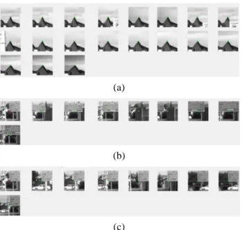
Figure 7. (a)An example of matching correctly, (b) An example of matching incorrectly, (c) Improperness of
incorrect matching by manual measurement
Figure 8. System error results in a discrepancy
5. CONCLUSIONS
This paper shows the feasibility of spatial positioning of interested points using MMS image sequences. The three problems, scale variations, different field of view, and occlusions, can be improved by matching in object space, rotating the assuming planes and conjugate image filtering respectively. Furthermore the influence of background can be reduced by multi-window matching.
This research utilizes two different data resource. One is for the real street view and the other is for the field with known control points. The correct matching is about 76% for street view. The failures are normally caused by the complex background and can all be improved by measuring conjugate points manually. For our developed MMS image sequences, the determined coordinates are about 10 cm in precision, and about 50 cm in accuracy. For these data within some system errors, the accuracy and precision are both accepted.
Table 1. Differences of 3D coordinate between the reference control points and the matching points
Number dX(m) dY(m) dZ(m) dS(m) D007 0.20 -0.24 -0.56 0.64 D010 0.09 0.27 -0.61 0.68 D019 -0.16 0.42 -0.53 0.70 D022 -0.07 0.30 -0.55 0.63 D025 0.12 0.17 -0.52 0.56 D040 0.02 -0.47 -0.55 0.72 D055 -0.01 -0.10 -0.20 0.23 D058 0.34 -0.08 -0.34 0.49 D061 0.38 -0.00 -0.42 0.56 D064 -0.12 -0.29 -0.26 0.41 D070 0.20 0.35 -0.44 0.60 D076 0.10 0.18 -0.38 0.43 D082 0.11 0.03 -0.40 0.41 D085 0.14 -0.05 -0.40 0.42 D097 0.04 -0.14 -0.50 0.52 D100 0.01 0.08 -0.30 0.32
Table 2. Mean, RMSE, std of the correct matching points dX dY dZ dS mean(m) 0.09 0.03 -0.43 0.52 RMSE(m) 0.17 0.24 0.45 0.54
std(m) 0.15 0.25 0.12 0.14
References:
El-Sheimy, N. 1996. The Development of VISAT – A Mobile Survey System for GIS Applications. Department of Geomatics Engineering. Calgary, Canad, the University of Calgary. Ph.D. thesis.
Lapucha, D. (1990). Precise GPS/INS Positioning for Highway Inventory System. Department of Geomatics Engineering. Calgary, Canada, The University of Calgary. M.Sc thesis.
McGlone, J. C. (2004). Manual of photogrammetry (fifth ed.): American Society for Photogrammetry amd Remote Sensing.
Wiman, H. (1998). Automatic generation of digital surface models through matching in object space. Photogrammetric Record 16(91): 83-91.
(a)
(b)
(c)
Projected
control point Control