Three-year Patch Thinning Effects on the Stand Structure in Overstory Trees of a Japanese Cedar Plantation in Taiwan
Dar-Hsiung Wang,
1,4)Chih-Hsin Chung,
1)Han-Ching Hsieh,
2)Shyh-Chian Tang,
1)Tsai-Huei Chen
3)【 Summary】
Stand structure plays an important role in forest ecosystem management. In this study, we examined the immediate and 3-yr effects of patch thinning treatments on the stand structure of overstory trees in a 35-yr-old Japanese cedar (Cryptomeria japonica) plantation located in the Zenlen area, central Taiwan. Among twelve 1-ha plots, 4 plots were randomly assigned to 1 of 3 patch thinning intensities in a randomized complete block design: no removal (control), and 25 and 50% tree removal in the area. The stand structure of the residual overstory trees was examined immediately after thinning and again after 3 yr using non-spatial stand structural indices (vertical evenness and the diameter at breast height (DBH) distribution), a pair correlation function (G func- tion), and spatial stand structural indices (diameter differentiation index and structural complexity index). The vertical evenness of the overstory tree canopy was reduced after thinning. Unlike the left-truncated Weibull DBH distribution commonly caused by thinning from below, no notable left-truncated Weibull distribution caused by patch thinning was detected. The change in the spatial point pattern expressed by the G function with scale-up at a distance scale was influenced by the intensity of the thinning. The stand structural complexity was affected by the spatial scale used and stand attributes surveyed, and it was reduced immediately after thinning but had varying impacts on the DBH and tree height.
Key words: vertical evenness, pair correlation function, stand structural complexity, Weibull func- tion, diameter differentiation index.
Wang DH, Chung CH, Hsieh HC, Tang SC, Chen TH. 2015. Three-year patch thinning effects on the stand structure in overstory trees of a Japanese cedar plantation in Taiwan. Taiwan J For Sci 30(1):55-74.
1)Division of Forest Management, Taiwan Forestry Research Institute, 53 Nanhai Rd., Taipei 10066, Taiwan. 林業試驗所森林經營組,10066台北市南海路53號。
2)Tamali Research Center, Taiwan Forestry Research Institute, 9-3 Choto Rd., Dawang Village, Taitung County 96341, Taiwan. 林業試驗所太麻里研究中心,96341台東縣太麻里鄉大王村橋頭9號 之3。
3)Division of Silviculture, Taiwan Forestry Research Institute, 53 Nanhai Rd., Taipei 10066, Taiwan.
林業試驗所育林組,10066台北市南海路53號。
4) Corresponding author, e-mail:[email protected] 通訊作者。
Received September 2014, Accepted March 2015. 2014年9月送審 2015年3月通過。
研究報告
塊狀疏伐對柳杉上層林木林分結構三年之影響
汪大雄
1,4)鍾智昕
1)謝漢欽
2)湯適謙
1)陳財輝
3)摘 要
林分結構在森林生態系經營中承擔重要之角色。本研究探討人倫地區35年生柳杉人工林在塊狀疏
伐後三年內對上層林木林分結構之影響。試驗地內設置12個1公頃樣區,進行上層林木之每木調查和樣
木位置之量測。以逢機區集方式逢機進行三種疏伐強度(疏伐面積25、50%和對照)之塊狀疏伐,每一
處理重複4次。使用垂直均勻、胸徑分佈、組對空間相關函數(G函數)、胸徑分化指標和結構複雜度指
標來推估疏伐後立即和前三年對林分上層木結構之影響。結果顯示上層林木之垂直均勻度在疏伐後降 低;和下層疏伐不同,塊狀疏伐在疏伐後不會造成胸徑分佈之明顯左截;尺度變化導致林木空間點分 佈,因疏伐強度之不同有所差異;林分結構複雜度隨者空間尺度和林分屬性有所變異,塊狀疏伐在疏 伐後立即降低林分結構複雜度,但對胸徑和樹高則有不同之影響。
關鍵詞:垂直均勻、組對空間相關函數、林分結構複雜度、胸徑分化指標。
汪大雄、鍾智昕、謝漢欽、湯適謙、陳財輝。2015。塊狀疏伐對柳杉上層林木林分結構三年之影響。
台灣林業科學30(1):55-74。
INTRODUCTION
In plantations, competition in the roots and crowns of trees occurs at the onset of crown closure. Crowded trees compete for light, water, and nutrients, resulting in the slow growth or even death of some trees (Oli- ver and Larson 1996). To avoid overcrowding and minimize negative effects of competition, trees are often thinned to increase the grow- ing space available for residual trees. There- fore, thinning is one of the most commonly employed forest silvicultural treatments used to enhance the growth of final crop trees (Ab- bott and Loneragan 1983).
Traditionally, the objective of thinning was to create more space or redistribute the resources available for residual trees, thereby, producing higher-quality sawlogs (Smith 1986, Mäkinen and Isomäki 2004). Recently, issues regarding biodiversity, environmental health, recreation, competing land use objec-
tives, carbon sequestration, and wildlife habi- tats have affected public attitudes towards forest management, and thinning has also been viewed as an important treatment for ad- dressing some of these issues (Sheriff 1996, Chambers et al. 1999).
In addition to effects on individual tree and stand growth (Marquis and Ernst 1991, Mäkinen and Isomäki 2004), thinning affects soil water availability (Donner and Running 1986), ecophysiology (Gauthier and Jacobs 2010), plant physiology, nutrient contents (Ginn et al. 1991, Bauhus et al. 2001), under- story plant communities (Dodson et al. 2008, Fahey and Puettmann 2008), the micorclimate environment (Della-Binanca and Dils 1960, Wang et al. 2003, Weng et al. 2007, Rambo and North 2009), and long-term tree mortality trends (Powers et al. 2010).
Tappeiner II et al. (2007) listed 5 types
of thinning that vary in the way trees are re- moved: (1) thinning from below; (2) thinning from above; (3) crown thinning; (4) free thin- ning; and (5) strip or row thinning. The result- ing average diameter at breast height (DBH) and crown size of residual trees differ with each type. For example, thinning from below is the most widely used type, where the aver- age DBH and crown size of the residual trees increase due to the removal of suppressed, intermediate, and smaller co-dominant trees.
In contrast, when thinning from above, the average DBH and crown size of residual trees decrease because of the removal of dominant and co-dominant trees. Even if the residual stocking levels are the same among the 5 types of thinning, different tree- and stand- level responses to thinning will result because attributes of the residual tree populations dif- fer (Weiskittel et al. 2011). Patch thinning, is actually thought to be thinning that does not account for tree size. It is similar to the row thinning method with the only difference be- ing in the shape and usually creates more gaps than those methods of thinning from below.
The forest structure is of interest to many disciplines and is often discussed in the con- text of ecosystem management. The forest structure encompasses many meanings and can be described in many ways (Pommerening 2002). Measurements of trees size, age, foli- age distribution, biomass, and spatial distri- bution in the overstory and ground vegetation layers are commonly viewed as components of stand structure (Spies 1998). At the stand level, the stand structure appears to be a good surrogate measure for biodiversity in forest ecosystems (Barbeito et al. 2009). The struc- ture of tree crowns, for example, is a charac- teristic of the stand structure that influences the growth of both trees and the understory vegetation (Latham et al. 1998). Changes in structural attributes of stands also affect
stand functions such as photosynthesis, res- piration (Waring and Schlesinger 1985), tree growth (O’Hara 1988), suitability of a stand for wildlife (Morrison et al. 1992, Mountford and Peterken 1999), and understory plant di- versity (Latham et al. 1998). Moreover, stand structure is also considered an important ele- ment of stand biodiversity (MacArthur and MacArthur 1961, Freemark and Merriam 1986, Staudhammer and LeMay 2001). Thus, in terms of ecosystem service and biodiver- sity, stand structural diversity has become an important facet within forestry, especially for countries with a rather low level of tree species diversity, such as those of the Central European Region (Neumann and Stalinger 2001).
The spatial forest structure influences growth processes, and all biotic and abiotic impacts modify the spatial structure (Zenner 2000). Several structural indices have been developed to quantify the spatial forest struc- ture and are used as surrogate measures for quantifying biodiversity (Zenner and Hibbs 2000, Gandow and Hui 2002, Pommeren- ing 2002, Barbeito et al. 2009). A good un- derstanding of the spatial forest structure is crucial for the sustainable management for economic and environmental purposes (Pom- merening 2006).
Taiwan is a mountainous island with an area of about 36,000 km2 in the South China Sea. The forests of Taiwan cover 58% of the island’s area, of which about 73% are consid- ered natural forests (TFB 1995). Japanese ce- dar (Cryptomeria japonica), also called sugi, was introduced to Taiwan by the Japanese government in 1921 based on its successful experiences in plantation establishment in Japan (Chao 2005). In 2000, sugi plantations were the second most common plantation species in Taiwan, with an area of 47,000 ha, accounting for about 22% of the total conifer
plantations in Taiwan (World Forest Institute 2001).
In the past, sugi plantations were planted as monocultures mainly for timber production in Taiwan. Nowadays, with the emphasis on forest ecosystem management, the concern has become how to apply thinning practices to existing sugi plantations to enhance the heterogeneity of the stand composition and structure so as to meet the goals of biodiver- sity conservation and promote land productiv- ity and stability of ecosystems for sustainable plantation management in Taiwan.
While there are studies investigating the thinning effects on sugi plantations in the past in Taiwan, they all used the approach of thinning from below to solely increase timber production (Weng et al. 2007, 2011, Yen et al. 2008). No patch thinning was examined in the field. As the overstory stand structure influences a wide range of ecosystem process, including wildlife abundance (Lehmkuhl et al. 2006), understory vegetation composition, and biomass (Collins et al. 2007), and being that patch thinning is a new approach adopted in Taiwan, the purpose of this study, there- fore, was to investigate the immediate and 3-yr influences of alternative patch thinning strate- gies on the structural diversity of overstory trees in a sugi plantation in the Zenlen area of central Taiwan.
MATERIALS AND METHODS Site description
The experiment site was in the 74th and 75th compartments of the Nan dai national working circle of the Taiwan Forestry Bureau, in the Zenlen area of central Taiwan. The sugi plantation was planted in 1971~1972 with an area of 78 ha at elevations of 1500~1700 m. Based on records from the nearby Sun- Moon Lake Weather Station (120°54’29”E,
23°52’53”N, elevation 1018 m), the mean an- nual precipitation at the study site is 3800 mm mostly in May to September. The mean an- nual temperature is 17.5℃. The average slope of the study area is 20o ~ 22o. The soil has a loamy sand (LS) type texture composed of 78.2% sand and 9.3% clay on average (Wang 2010, pers. comm).
Experimental design and thinning treat- ments
A randomized block design was used that had 3 thinning intensities, replicated 4 times on 1-ha plots. All 12 plots were uniform in topography and aspect. A buffer strip, 20~30 m in width, separated each plot. The total area of the sugi plantation for the experiment was about 25~30 ha.
In each plot, stems of all woody plants with a DBH of > 1 cm were tagged, identi- fied by species, and measured for DBH. Stem location was recorded on a Cartesian coordi- nate system. Height was measured on trees sampled across the range of DBH to develop a DBH-height curve for sugi.
Thinning was accomplished by remov- ing all overstory trees within patches 10×10 m in size. The patches were systematically located to cover 25 or 50% of the total area of a plot. For the 25% thinning intensity, 1 patch located in the lower-left corner was cut within each of 25 quadrants with dimensions of 20×20 m (Fig. 1). For the 50% thinning intensity, 2 patches connected southwest to northeast diagonally were cut within each quadrant (Fig. 1).
Functions and indices of the stand struc- ture
In this study, both spatially implicit and spatially explicit functions and stand struc- tural indices were used to assess the impacts of patch thinning on the stand structure.
Spatially implicit stand structural indi- ces
Indices were developed to assess the ver- tical and horizontal components of the stand structure. Five canopy layers of sugi tree heights (< 13, 13~15, 15~17, 17~19, and > 19 m) were used to calculate the vertical even- ness (VE; Equ. 1). The 3-paramater Weibull function (Bailey and Dell 1973) was used to estimate the DBH distribution among tress because of its modeling flexibility and easy computation (Lynch and Moser 1986, Zhang et al. 1993):
VE = (-log p)×p/log 5; (1)
where p is the ratio of the number of trees for a given class i to the total number of trees.
Function and spatially explicit stand structural indices
In addition to indices or empirical dis- tributions, functions are also used to model point processes in statistics (Penttinen et al.
1992). The pair correlation function used in this study was the G function (Zhukov 2010).
The G function in this study measures the dis- tribution of distances from an arbitrary tree to its nearest neighbors :
g^(r) = ; (2)
where
li =
{
1 If di {di : di ≤ r, i}0 otherwise
di is the distance between the subject tree i Fig. 1. Allocation of cutting areas indicated by dark slashes for a thinning intensity of 25 in area. Two 1/4 quadrants (10×10 m) diagonally connected southwest to northeast within a 20×20-m block were set up as the cutting area for a thinning intensity of 50 .
to its nearest neighbor tree j; r is a given dis- tance; and n is the number of subject trees.
Unlike the aggregation index, R (Clark and Evans 1954), the pair correlation func- tion g(r) does not result in 1 number, but in a function which can be plotted on a graph.
The comparability of point processes with complete spatial randomness (CSR) can be assessed by plotting the empirical function (i.e., observed value) against the theoretical expectation, G(r). For a regular pattern, val- ues of the empirical function are below envel- ops, and a contrast exists for a cluster pattern (Zhukov 2010).
The diameter differentiation index (Pom- merening 2002), based on the nearest neigh- boring tree distance, was applied to spatially express size differences of neighboring trees on a continuous scale. For the ith reference tree and its n = 3 nearest neighboring trees j (j
= 1…n), the diameter differentiation index Tij is defined as:
Tij = 1 - [min (DBHi, DBHj) / max (DBHi,
DBHj)] ; (3)
where DBH is the diameter at breast height (in cm).
To calculate the diameter differentiation of an entire stand, all Tij values are summed and divided by the number of trees to obtain a single number, T. Diameter differentia- tion values can be classified as follows. (1) A small differentiation comprises the class 0.0~0.3 indicating that the tree with the small- est DBH is ≧ 70% of the neighboring tree’s size. (2) An average differentiation comprises the class 0.3~0.5 which means that the tree with the smallest DBH is 50~70% of that of the neighboring tree. (3) A big differentiation comprises the class 0.5~0.7 indicating that the tree with the smallest DBH is 30~50% of the neighboring tree’s size. (4) A very big differ- entiation comprises the class 0.7~1.0 which means that the tree with the smallest DBH is
< 30% of the neighboring tree’s size (Pom- merening 2002).
Based on vertical gradients and distances of neighboring trees, Zenner and Hibbs (2000), using the triangular irregular network (TIN) (Fig. 2), created an index called Struc- tural Complexity Index (SCI) to measure structural variability among stands.
The SCI is defined as the sum of the surface areas of the TINs for a stand (SAT) divided by the ground area covered by all tri- angles:
SCI = SAT / AT; (4)
where AT is the sum of the projected areas of all triangles and SAT = |ai×bi|, i = 1,..., N, N is the number of triangles in the plot,
|ai×bi| is the absolute value of the product of the vector AB with coordinates ai = (xib–xia, yib–yia, zib–zia) and the vector AC with co- ordinates bi = (xic–xia, yic–yia, zic–zia) (Fig.
2). The sum of 1/2 the vector products gives a surface area in 3 dimensions by connecting the z-coordinates of trees with spatial coordinates x and y. When all trees in a stand have the same z (e.g., height), the value of SCI equals 1, giving the lower limit of the SCI (i.e., when all trees in a stand have the same height).
In order to investigate the scale impact on the SCI, 2 scales were used in this study.
One scale regarded the entire plot as a unit (i.e., 100×100 m), and calculated 1 value for each plot. The other divided the entire plot into 100 subunits of 10×10 m in size, then calculated the SCI for each subunit, and aver- aged the subunit SCI values to obtan 1 value for each plot.
Edge correction
Indices accounting for tree positions re- quire an edge correction process (Pommeren- ing and Stoyan 2006) to avoid an edge bias in index calculations. In this study, we used
the buffer method (Diggle 2003) for which only trees within a buffer strip of 10 m along the plot boundaries (i.e., the inner part of size 80×80 m) were used to calculate the SCI on both small and large scales.
RESULTS
Stand structural characteristics
The stand density of overstory trees
ranged from 893~1285 trees/ha, and the aver- age DBH varied 24.1~27.8 cm among plots (Table 1). Competition among trees and other factors may account for the heterogeneity among plantations. Computation of the spe- cies composition in basal area showed that sugi and China fir (Cunninghmia lanceolata) were the dominant overstory trees in the stand. Because the basal area of sugi was >
80% of the total basal area in the overstory Fig. 2. Structral Complexity Index Delaunay triangulation for plots 1 (above) and 2 (below) before (left) and after thinning (right) on the 80×80-m scale.
layer, the plantation was still considered a pure sugi plantation.
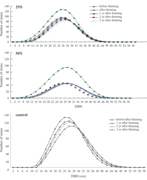
Thinning effects on the stand structure Comparisons of stand attributes showed that the thinning intensity in terms of the area treated can be roughly applied to the number of trees, basal area, and volume removed (Table 2). The Weibull DBH distribution of each plot approximated a normal distribution, and its shape did not change after thinning regardless of the thinning intensity, as shown, for example, by plots 11 and 5 (Fig. 3). In the control plot, the shape of Weibul distribution gradually shifted downwards revealing the in- creasing mortality of trees over time (Fig. 3).
In each plot, the DBH differentiation index was compared before and 0~3 yr af- ter thinning. Before thinning, using plot 11, where removal of trees within 25% of the area, was scheduled, as an example, we found that most trees expressed a DBH difference with their neighbors that varied spatially in the ‘small level’ (0.0~0.3), meaning that DBH differences among neighboring trees were <
30%. Only a few trees differed in DBH by
> 50% from their neighbors, i.e., at the ‘big level’ of differentiation (Fig. 4). However, the percentage of trees with a DBH differentia- tion index at the ‘small level’ increased after thinning (65 to 72%). On the contrary, the percentage of trees with a DBH differentiation index of an ‘average level’ decreased after thinning (27 to 23%). The same pattern of the DBH differentiation index was observed in plot 5 with the 50% thinning intensity (Fig. 4).
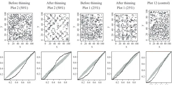
The spatial pattern of plots can be ob- served using the G function. The G function measures the distribution of distances from an arbitrary event to its nearest events (Ripley 1988). In this study, under the relative dis- tance (i.e., distance observed / distance of the plot boundary) framework, for a given relative distance (e.g., 0.2), we calculated the proportionality of trees in a plot which had a distance to their nearest neighbors of less than or equal to a given relative distance, and then we judged the spatial point pattern based on a comparison of the empirical function G(r) to its G function under the CSR. The resulting G Table 1. Characteristics of stand attributes for overstory trees surveyed on a 1-ha basis in the study area
Plot Density DBH Height Basal area Volume
(no. of stems) (cm)a) (m)a) (m2 ha-1) (m3 ha-1)
1 893 27.0±7.3 17.48±1.99 54.77 461.45
2 944 27.6±7.5 17.62±1.70 60.63 512.10
3 1055 26.0±6.3 17.37±1.45 58.39 488.86
4 939 27.8±6.9 17.72±1.63 60.57 511.86
5 895 25.2±6.9 17.15±1.85 47.88 400.10
6 1114 26.5±6.6 17.49±1.56 65.32 548.84
7 1285 24.1±6.3 16.98±1.61 62.79 520.77
8 1019 25.6±5.8 17.37±1.41 55.24 461.92
9 1184 24.2±6.4 16.98±1.59 58.32 484.17
10 964 27.5±7.1 17.64±1.57 61.01 514.90
11 1074 24.3±6.3 17.00±1.70 52.92 439.60
12 896 26.3±7.2 17.38±1.66 52.28 439.05
a)Mean±standard deviation.
DBH, diameter at breast height.
function showed that the point pattern of the tree spatial distribution vaied depending on the spatial scale used (Fig. 5).
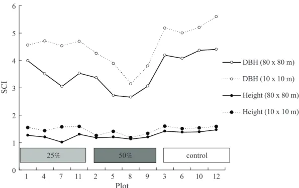
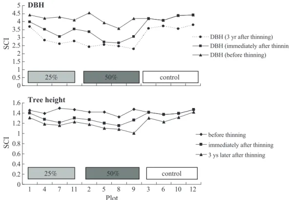
The SCI is an index which can be used to describe the structural complexity of DBH or tree height in a 3D format. Regarding the 2 scales used in computing the SCI, theoreti- cally, the more homogenously distributed the spatial point is, the closer these 2 scales of the SCI should be. This study showed a tendency that because of the heterogeneity of the point spatial pattern in the plot (Fig. 2), the SCI obtained at the small scale (10×10 m) was greater than that obtained at the larger scale (80×80 m) for each plot before thinning in terms of both the DBH and tree height struc- tural complexity (Fig. 6). However, the differ- ence between the 2 scales was reduced after thinning (Fig. 7). Moreover, for a larger scale, thinning will reduce the structural complexity for both attributes, but with different impacts between them (Fig. 8). The change of the SCI in the short-term reveals that the SCI was decreasing over time even in the control plots (Fig. 9).
DISCUSSION
Stand density and structure
In general, the percentage of area, num-
ber of stems, and basal area or tree volume are often used to express thinning intensities (Knoebel et al. 1986, Pukkala et al. 1998, Mäkinen and Isomäki 2004,). Nevertheless, the same figure expressed by a different cri- terion often conveys a different meaning. For example, thinning from below extracts the suppressed, intermediate and smaller codomi- nant trees. Those trees contribute a smaller proportion to the stand basal area and volume;
hence, a given thinning intensity expressed as a percentage of the number of trees will leave a very different residual stand compared to one in which the same percentage is applied to removing the basal area or tree volume (Weiskittel et al. 2011). In this study, however, because of the systematic allocation of the cutting area (Fig. 1), although heterogeneity in stand attributes exists among plots (Table 1), all overstory trees in the cutting area were re- moved. Because of their relatively even distri- bution over the study area, the same percent- age for the thinning intensity in patch thinning can be roughly applied to the area, number of trees, basal area, and tree volume (Table 2).
Patch thinning used in this study ig- nores tree species, tree size, and crown class by selecting trees for removal based solely upon whether the tree is located in the patch that is allocated for cutting. Therefore, patch Table 2. Comparisons of stand attributes between before and after thinning by plot
Treatment Number of trees (ha) Basal area (m2 ha-1) Volume (m3 ha-1) plot
area (ha) Before
Removed Percent Before
Removed Percent Before
Removed Percent thinning removed thinning removed thinning removed 1 0.25 893 264 29.6 54.77 15.28 27.9 461.45 128.28 27.8 4 0.25 939 239 25.4 60.57 15.02 24.8 511.86 126.43 24.7 7 0.25 1285 253 19.7 62.79 12.81 20.4 520.77 106.76 20.5 11 0.25 1074 270 25.1 52.92 12.44 23.5 439.60 102.43 23.3 2 0.50 944 507 53.7 60.63 31.40 51.8 512.10 264.24 51.6 5 0.50 895 490 54.8 47.88 26.24 54.8 400.10 219.25 54.8 8 0.50 1019 494 48.5 55.24 26.51 48.0 461.92 221.26 47.9 9 0.50 1184 596 50.3 58.32 28.86 49.5 484.17 239.18 49.4
thinning can be regarded as a type of strip or row thinning (Weiskittel et al. 2011).
An earlier study on the same site showed that in addition to the dominant overstory species of sugi and China fir, several broad- leaf species occur as the understory woody vegetation. While the basal area shared by
understory woody plants was quite small in the plantation (i.e., < 5%), an enhancement of biodiversity was obvious. The biologi- cal diversity (Shannon diversity index) of all woody plants increased after thinning, but there was little change in overstory trees (Wang et al. 2011).
Fig. 3. Diameter at breast height (DBH) distribution for plot 11 with a 25 thinning intensity, plot 5 with a 50 thinning intensity, and plot 3 with no treatment (control).
25
50
control
Effects of thinning on the vertical and horizontal structure
Vertical structure plays an important role in forest ecosystems (North et al. 1999, Barbeito et al. 2009). Analyzing spatial pat- terns within different tree height classes can provide many important clues about the un- derlying processes that have generated those patterns (Zenner and Hibbs 2000) Using the same categories of canopy layers as used in this study, Wang et al. (2011) demonstrated that, while little difference was found among plots, the evenness index value was > 0.5
for all plots before thinning, and the vertical evenness of the canopy was slightly reduced immediately after patch thinning for all thinning intensities adopted with the same as these used in our study. Moreover, this study showed that no significant difference in vertical evenness existed even when the understory trees (i.e., broadleaf trees) were included (1-sample t- test n = 12, p = 0.152).
This is because all understory trees were < 13 m in height, and their inclusion did not make a notable change in vertical evenness index values. As the residual trees and understory Fig. 4. Distribution of the diameter at breast height (DBH) differentiation index based on the first nearest neighboring distance with 25 (plot 11) and 50 of the thinning intensity (plot 5).
0
0.2 0.2 0.2 0.2
0.2
0.2 0.2 0.2 0.2
0.2
0 0 0 0
80 80 80 80 80
60
0.8 0.8 0.8 0.8
0.8
0.8 0.8 0.8 0.8 0.8
60 60 60 60
40
0.6 0.6 0.6 0.6
0.6
0.6 0.6 0.6 0.6 0.6
40 40 40 40
20
0.4 0.4 0.4 0.4
0.4
0.4 0.4 0.4 0.4 0.4
20 20 20 20
100 100 100 100 100
0 0 0 0 0
80 80 80 80 80
60 60 60 60 60
40 40 40 40 40
20 20 20 20 20
100 100 100 100 100
x x x x x
y y y y y
woody plants will grow over time, it is ex- pected that the resulting vertical evenness structure will gradually recover.
The stand horizontal structure in DBH distribution will be affected by thinning op-
erations. As discussed, the change in the DBH distribution depends on the thinning type used, such as thinning from below where the diameter distribution is notably left-truncated after thinning because trees of a small size Fig. 5. G function for plots before and after the thinning practice for thinning intensities of 25 and 50 .
Fig. 6. Comparisons of the Structural Complexity Index (SCI) for diameter at breast height (DBH) and height on 2 scales (80×80 vs. 10×10 m) for 12 plots before thinning. Plots 1, 4, 7, and 11 had a thinning intensity of 25 ; plots 2, 5, 8, and 9 had a thinning intensity of 50 , and plots 3, 6, 10, and 12 were controls.
Before thinning
Plot 2 (50%) After thinning
Plot 2 (50%) Before thinning
Plot 1 (25%) After thinning
Plot 1 (25%) Plot 12 (control)
Fig. 7. Comparisons of the Structural Complexity Index (SCI) for diameter at breast height (DBH) and height on 2 scales (80×80 vs. 10×10 m) for 12 plots after thinning. Plots 1, 4, 7, and 11 had a thinning intensity of 25 ; plots 2, 5, 8, and 9 had a thinning intensity of 50 , and plots 3, 6, 10, and 12 were controls.
Fig. 8. Changes in the Structural Complexity Index (SCI) for diameter at breast height (DBH) and height on the 80×80-m scale before and after thinning. Plots 1, 4, 7, and 11 had a thinning intensity of 25 ; plots 2, 5, 8, and 9 had a thinning intensity of 50 ; and plots 3, 6, 10, and 12 were controls.
Fig. 9. Changes in the Structural Complexity Index (SCI) for diameter at breast height (DBH) and tree height over 3 yr after thinning on the 80×80-m scale. Plots 1, 4, 7, and 11 had a thinning intensity of 25 ; plots 2, 5, 8, and 9 had a thinning intensity of 50 , and plots 3, 6, 10, and 12 were controls.
or suppressed trees are removed (Wang et al.
2003, 2006, Li and Yen 2010). However, un- der systematic patch thinning, the DBH dis- tribution type depends on the spatial distribu- tion of small trees and their location relative to the cutting area. If fairly uniform, only a slight truncation of the tree diameter distribu- tion after thinning would exist, as observed in this study (Fig. 3). Among the treated plots in this study, almost each plot showed a non- or slightly truncated DBH distribution after thinning. This finding was valid regardless of the thinning intensity adopted (Fig. 3). As mentioned earlier, patch thinning is a type of row thinning, and this finding for the DBH structure confirms that in row thinning, the average DBH, crown size, and species com-
position of the residual trees should remain the same as those of the stand as a whole be- fore thinning (Weiskittel et al. 2011).
Thinning effects on function and spatial indices of the stand structure
Just like Gadow’s differentiation index used by Barbeito et al. (2009) for the tree height distribution, Pommerening’s DBH differentiation index (Pommerening 2002) can be used to measure small-scale spatial variabilities in the DBH size distribution.
Thinning impacts on the DBH differentiation index pattern depend on the method used for thinning. In traditional thinning from below, as the removed trees are concentrated on small trees and suppressed trees, thus narrow-
ing the range of residual trees, the proportion of the DBH differentiation that falls at the
‘small level’ substantially increases (Wang et al. 2006). However, in this study, as all over- story trees were removed regardless of size, the range of DBH for residual trees did not shrink as rapidly, and therefore, the DBH dif- ferentiation pattern at various levels did not notably change by and thinning practice. This pattern was not influenced by the thinning in- tensity (Fig. 4). Moreover, over 3 yr, the pat- tern of the DBH differentiation index among different levels did not remarkably change for either intensity.
Interpretation of the point pattern ex- pressed by the G function for a given plot varies depending on the spatial distance scale used in a plantation. At a small distance scale (e.g., 0.2 or 0.4), the point pattern is regarded as a regular pattern; however, at a larger distance scale (i.e., > 0.8), the point pattern shifts toward a randomized pattern (Fig. 5).
Specifically, the type of point pattern for a given subject relies on the spatial scale used.
The trend of the point pattern going from a small distance level to a large distance level expressed by the G function is affected by thinning, and the direction of change is influenced by the intensity of thinning used (Fig. 5). At the lower thinning intensity, for example, the distance scale at which the point pattern remained regular was reduced from 0.8 to 0.4 after thinning. This reduction in the distance scale became larger in the case of the higher thinning intensity (e.g., from 0.8 to 0.3 for the 50% intensity). Moreover, the point pattern change at a larger distance scale was also influenced by the intensity of thinning employed. At the lower intensity, the trend of the point pattern over the distance scale moved from regular to randomized. But, at the higher thinning intensity, the sequence of this change was from regular to random and
then to clustered (Fig. 5). Based on a distance scale of 0.5, all plots were viewed as regularly spatially distributed before thinning; however after thinning, plots with the 25% intensity were viewed as being randomly distributed, and plots with the 50% intensity had a cluster distribution (Fig. 5).
The SCI depends on the spatial scale used (Zenner and Hibbs 2000), and this study showed the difference in the SCI between 2 scales. The SCI obtained from the small scale was greater than that obtained with the larger scale for each plot before thinning, because there was quite a variety in the SCI among subunits (Figs. 2, 6). However, these differences in the SCI between the 2 scales were reduced after thinning (Fig. 7). This is because all overstory trees in the cutting area (10×10 m) were removed, and the SCI for these areas was reduced to 1, thus reducing the average value of the SCI. The narrowing of the difference was more apparent for the case of thinning at 50%. In other words, the impacts on the SCI caused by the spatial scale gradually vanished after thinning (Fig. 7).
As the SCI is calculated based on the gradient surface among trees, the range and standard deviation of the DBH or height (z) will influence the SCI value. Since the stand deviation of the DBH in our study was much greater than that of tree height (Table 1), the SCI for DBH was, therefore, bigger than the tree height SCI (Fig. 6). In other words, low SCI values for tree height indicated that these plots were extremely homogeneous in terms of the tree spatial vertical complexity struc- ture. On the contrary, a higher SCI values for DBH meant that a much higher heterogeneity existed in the tree horizontal spatial complex- ity structure.
In an earlier study, the SCI was used to evaluate the DBH structural complexity of Douglas fir-dominated mixed conifer stands
in the west-central Cascades of Oregon, USA (Zenner 2004). Compared to this study, SCI values in Zenner’s study were much higher than those we obtained. For example, the highest SCI in Zenner’s study was 13.34 compared to the highest SCI of 5.8 for diam- eter structural complexity seen here (Fig. 6).
This is because the stands studied in Oregon ranged from natural mature (80~150 yr old) to old growth (> 150 yr old) in contrast to the quite young (< 40 yr old) and higher-density plantation examined in this study (Table 1).
In old-growth forests, a higher SCI exists be- cause diameter distributions reflect the mul- tiple pathways of development resulting from complex regional disturbance regimes (Spies and Franklin 1991, Spies 1998).
The lack of a correlation of the diameter SCI with tree density (p = 0.655) and mean DBH (p = 0.194) shown in our study closely mirrors results in evaluating the relationship of the index of old-growth structure with tree density and average DBH as reported by Acker et al. (1998). A stronger positive asso- ciation between the SCI and the standard de- viation of the DBH (p = 0.003) in this study confirms that a large variation in tree sizes is an important requirement for higher structural complexity (Zenner 2004).
The SCI for the DBH of all plots did not significantly differ among treatments before thinning (F = 0.71, p = 0.518, Fig. 8); how- ever, a significant difference occurred among treatments after thinning (F = 36.5, p = 0.000, Fig. 8). Among them, the average SCI for the DBH of the control was highest (4.2514), fol- lowed by the DBH SCI for the 25% thinning intensity (3.8014), and then by that for the 50% thinning intensity (3.0335).
While a high variability in tree sizes is a necessary condition for higher structural complexity, the processes influencing spa- tial patterns of differently sized trees (e.g.,
thinning) ultimately determine the extent of structure complexity (Zenner and Hibbs 2000, Zenner 2004). Our study shows that the stand structural complexity was reduced by thinning, just like the case of thinning from below (Barbeito et al. 2009). The reason for the lower SCI caused by thinning is that after thinning, the complexity of the structure in the cut area was lost due to the removal of all overstory trees, and this consequently re- duced the structure complexity of the entire plot. With a greater area cut, more structure complexity will be lost (Fig. 8).
Impacts on the SCI caused by thinning varied among stand attributes (Fig. 8). Com- pared to the SCI for the DBH, the change in the SCI caused by thinning on tree height was quite small. This is because the coefficient of variation (CV) of tree height in each plot was quite small before thinning (Table 1), and no notable change occurred after thinning (Table 3). Nevertheless, the CV for the DBH in each plot was higher than that for tree height both before and after thinning; thus, the reduction of the SCI for the DBH was more substan- tial than that for tree height. This finding is consistent with the result reported by Zenner (2004) that a higher SCI for the DBH struc- tural complexity was associated with a greater CV ranging from 48 to 98% for the DBH.
The trend of the SCI over time is also of interest. In a comparison of the SCI immedi- ately after thinning and at 3 yr after thinning, even that of the control plot was reduced after 3 yr (Fig. 9). A paired t-test showed that for all plots, a significant difference in the SCI existed 3 yr after thinning for DBH (t = 4.36, p = 0.001) and tree height (t = 5.35, p <
0.0001). The probable reason for this reduc- tion may have been the decrease in the CV for both attributes over 3 yr for all plots (Table 3).
However, longer observation periods will be required to see the trend of the SCI over time.
In the absence of tree height data, just like the height-DBH curve, the SCI for tree height can be estimated by the SCI for the DBH. In our case, the SCI for tree height = 0.689 + 0.1556 SCI for the DBH, with n = 12, R2 = 0.60 at the 80×80-m scale. This confirms that greater SCI values for the tree height also means greater SCI values for the DBH as reported by Zenner (2000).
CONCLUSIONS
This study showed the immediate and 3-yr effects of patch thinning on the stand structure of overstory trees in a sugi planta- tion. Several stand structure indices were used to measure the stand structural com- plexity and evaluate the short-term impacts on the stand structure caused by patch thin-
ning. Based on the ecosystem management approach to sugi plantations in Taiwan, this study provides an understanding of short- term changes to overstory stand structures fol- lowing patch thinning. However, longer-term monitoring of the dynamics of the structure indices examined in this study is still needed to evaluate the dynamics of patch thinning on the stand structural complexity as the stands develop. While it is beyond the scope of this study, the impact on the biodiversity and structural diversity of the understory trees due to patch thinning will be studied in the future.
ACKNOWLEDGEMENTS
The authors thank colleagues at the Lie- huahchi Research Center, Taiwan Forestry Research Institute for their help with the field work. This study was supported by financial assistance from the National Science Council, Taiwan, ROC (NSC992621M054001).
LITERATURE CITED
Abbott L, Loneragan O. 1983. Response of Jarrah (Eucalyptua marginata) regrowth to thinning. Aust For Res 13:217-9.
Acker SA, Sabin TE, Ganio LM, Mckee WA. 1998. Development of old-growth struc- ture and timber volume growth trends in ma- turing Douglas-fir stands. For Ecol Manage 104:265-80.
Bailey RL, Dell TR. 1973. Quantify diameter distribution with the Weibull function. For Sci 19:97-104.
Barbeito I, Canellsa I, Montes F. 2009. Eval- uating the behavior of vertical structure indices in Scots pine forests. Ann For Sci 66:710 p1- 10.
Bauhus J, Aubin I, Messier C, Connell M.
2001. Composition, structure, light attenu- ation and nutrient content of the understory Table 3. Characteristics of the diameter
at breast height (DBH) and tree height for overstory residual trees immediately after and 3 yr after thinning
Plot DBH (cm)a) Height (m)a) 1 25.8±6.8b) 17.0±1.4b)
29.6±7.5c) 18.0±1.4c)
2 27.0±7.3 17.5±1.5
30.7±7.7 18.2±1.2
4 27.2±6.7 17.5±1.4
29.2±7.0 18.0±1.3
5 25.0±6.8 17.1±1.8
26.6±6.5 17.5±1.4
7 24.5±6.2 17.0±1.6
25.5±6.2 17.3±1.5
8 25.5±5.7 17.4±1.4
27.5±6.0 17.8±1.1
9 24.0±6.2 17.0±1.5
27.1±7.0 17.6±1.3
11 23.3±6.2 16.6±1.5
26.4±6.2 17.5±1.3
a)Mean±standard deviation.
b)Immediately after the thinning operation.
c)Three years after the thinning operation.
vegetation in a Eucalyptus sieberi regrowth stands 6 years after thinning and fertilization.
For Ecol Manage 144:275-86.
Chambers CL, Mccomb WC, Tappeiner JC.
1999. Breeding bird response to three silvicul- tural treatments in the Oregon Coast Range.
Ecol Appl 9:171-85.
Chao KM. 2005. Forestry policy and adminis- tration. Taipei, Taiwan: Huanglei Publications.
250 p. [in Chinese].
Clark PJ, Evans FC. 1954. Distance to near- est neighbor as a measure of spatial relation- ships in populations. Ecology 35:445-53.
Collins BM, Moghaddas JJ, Stephens SL.
2007. Initial changes in forest structure and understory pant communities following fuel reduction activity in a Sierra Nevada mixed conifer forest. For Ecol Manage 239:102-11.
Della-Bianca L, Dils RE. 1960. Some effects of stand density in a red pine plantation on soil moisture, soil temperature and radial growth. J For 58:373-7.
Diggle PJ. 2003. Statistical analysis of spatial point patterns. 2nd ed. London: Arnold. 159 p.
Dodson EK, Peterson DW, Harrod RJ.
2008. Understory vegetation response to thin- ning and burning restoration treatments in dry conifer forest of the eastern Cascades, USA.
For Ecol Manage 255:3130-40.
Donner BL, Running SW. 1986. Water stress response after thinning Pinus contorta stands in Montana. For Sci 32:614-25.
Fahey RT, Puettmann KJ. 2008. Patterns in spatial extent of gap influence on understory plant communities. For Ecol Manage 255:
2801-10.
Freemark KE, Merriam HG. 1986. Impor- tance of area and habit heterogeneity to bird assemblages in temperate forest fragments.
Biol Conserv 36:115-41.
Gandow KV, Hui G. 2002. Characterizing forest spatial structure and diversity. In: Bjoerk L, editor. Proceedings of the IUFRO Interna-
tional Workshop Sustainable Forestry in Tem- perate Regions. Sweden: Lund. p 20-30.
Gauthier MM, Jacobs DF. 2010. Ecophysi- ological responses of black walnut (Juglans nigra) to plantation thinning along a vertical canopy gradient. Fort Ecol Manage 259:867- 74.
Ginn SE, Seiler JR, Cazell BH, Kreh RE.
1991. Physiological and growth responses of eight-year-old loblolly pine stands to thinning.
For Sci 37:1030-40.
Knoebel BR, Burkhart HE, Beck DE. 1986.
A growth and yield model for thinned stands of yellow-poplar. For Sci Monogr 27:62.
Latham PA, Zuuring HR, Coble DW. 1998.
A method for quantifying vertical forest struc- ture. Fort Ecol Manage 104:157-70.
Lehmkuhl JF, Kistler KD, Begley JS, Bou- langer J. 2006. Demography of northern fly- ing squirrels informs ecosystem management of western interior forests. Ecol Appl 16:584- 600.
Li LE, Yen TM. 2010. Thinning effects on stand and tree levels of Taiwan red cypress (Chamaecyparis formosensis) 4 years after thinning. Q J Chin For 43:249-60. [in Chinese with English Summary].
Lynch TB, Moser Jr. JW 1986. A growth model for mixed species stands. For Sci 32:
697-706.
MacArthur RH, MacArthur JW. 1961. On bird species diversity. Ecology 42:594-8.
Mäkinen H, Isomäki A. 2004. Thinning in- tensity and growth of Scots pine stands in Fin- land. For Ecol Manage 201:311-25.
Marquis DA, Ernst RL. 1991. The effects of stand structure after thinning on the growth of an Allegheny hardwood stand. For Sci 37:1182- 200.
Morrison ML, Marcot BG, Mannan RW.
1992. Wildlife-habitat relationships. Madison, WI: Univ. of Wisconsin Press. 343 p.
Mountford EP, Peterken GF. 1999. Effects
of stand structure, composition and treatment on bark-stripping of beech by grey squirrels.
Forestry 72:379-86.
Neumann M, Stalinger F. 2001. The signifi- cance of different indices for stand structure and diversity in forest. For Ecol Manage 145:
91-106.
North MP, Franklin JF, Carey AB, Forsman ED, Hamer T. 1999. Forest stand structure of the Northern Spotted Owl’s foraging habitat.
For Sci 45:520-7.
O’Hara KL. 1988. Stand structure and grow- ing space efficiency following thinning in an even-aged Douglas-fir stand. Can J For Res 18:859-66.
Oliver CD, Larson BC. 1996. Forest stand dynamics. New York: Wiley. 520 p.
Penttinen A, Stoyan D, Henttonen HM. 1992.
Marked point processes in forest statistics. For Sci 38:806-24.
Pommerening A. 2002. Approaches to quanti- fying forest structures. Forestry 75:305-24.
Pommerening A. 2006. Evaluating structural indices by reversing forest structural analysis.
For Ecol Manage 224:266-77.
Pommerening A, Stoyan D. 2006. Edge-cor- rection needs in estimating indices of spatial forest structure. Can J For Res 36:1723-39.
Powers MD, Palik BJ, Brandford JB, Frav- er S, Webster CR. 2010. Thinning method and intensity influence long-term mortality trends in a red pine forest. For Ecol Manage 260:1138-48.
Pukkala T, Miina J, Kellomäke S. 1998.
Response to different thinning intensities in young Pinus sylvestris. Scand J For Res 13:
141-50.
Rambo TR, North MP. 2009. Canopy mi- croclimate response to pattern and density of thinning in a Sierra Nevada forest. For Ecol Manage 257:435-42.
Ripley BD. 1988. Statistical inference for spatial processes. Cambridge, UK: Cambridge
Univ. Press. 160 p.
Sheriff DW. 1996. Responses of carbon gain and growth of Pinus radiata stands to thinning and fertilizing. Tree Physiol 16:527-36.
Smith DM. 1986. The practice of silvilculture.
New York: Wiley. 527 p.
Spies TA. 1998. Forest structure: a key to the ecosystem. Northwest Sci 72:34-9.
Spies TA, Franklin JF. 1991. The structural of nature young, mature, and old growth forests in Washington and Oregon. In: Ruggiero LF, Aubry KB, Carey AB, Huff MH, editors. Wild- life and vegetation of unmanaged Douglas-fir forests. USDA. Forest Service, PNW-GTR- 285. p 91-121.
Staudhammer CL, LeMay VM. 2001. Intro- duction and evaluation of possible indices of stand structural diversity. Can J For Res 31:
1105-15.
Tappeiner II JC, Maquire DA, Harrington TB. 2007. Silviculture and ecology. Western US forests. Corvallis, OR: Oregon State Univ.
416 p.
TFB. 1995. The third forest resources and land use inventory in Taiwan. Taipei, Taiwan:
Taiwan Forestry Bureau (TFB). 258 p. [in Chi- nese].
Wang DH, Chiu CM, Hsieh HC, Tang SL, Tang SC, Liu CK. 2003. Investigation on stand structure and microsite condition on Taiwania plantation prior to the secondary thinning practices in Liu-kuei Experimental Forest. Q J Chin For 36:1-16. [in Chinese with English Summary].
Wang DH, Chung CH, Hsieh HC, Tang SC, Chen TH. 2011. Baseline survey and immedi- ate thinning impact on the stand composition of woody plants and overstory structure of a sugi plantation (Cryptomeria japonica) in the Zenlen area. Taiwan J For Sci 26:295-303.
Wang DH, Tang SC, Chiu CM. 2006. Impact four years after thinning on the growth and stand structure of Taiwania plantation in the
Liukuei Experimental Forests. Taiwan J For Sci 21:339-51.
Waring RH, Schlesinger WH. 1985. Forest ecosystems: concepts and management. Or- lando, FL: Academic Press. 340 p.
Weiskittel AR, Hann DW, Kershaw Jr JA, Vanclay JK. 2011. Forest growth and yield modeling. Hoboken, NJ: Wiley-Blackwell.
415 p.
Weng SH, Kuo SR, Guan BT, Chang TY, Hsu HW, Shen CW. 2007. Microclimate re- sponse to different thinning intensities in a Japanese cedar plantation of northern Taiwan.
For Ecol Manage 241:91-100.
Weng SH, Shen CW, You CH, Lin CY, Chung NJ, Chen PY, Kuo SR. 2011. Effects of thinning on growth and structure of oversto- ry and understory woody plants of a Japanese cedar plantation in northern Taiwan. Q J Chin For 44:157-82. [in Chinese with English Sum- mary].
World Forest Institute. 2001. Taiwan’s forest sector. A WFI Market Brief Series, Portland, OR. Available at: http://wfi.worldforestry.org/
media/publications/marketbriefs/Taiwan_brief.
pdf.
Yen TM, Lee JS, Huang KL. 2008. Growth and yield models for thinning demonstration zones of Taiwan red cypress (Chamaecyparis formosensis) and Japanese cedar (Cryptomeria japonica) plantations in central Taiwan. Q J Chin For 30:31-40. [in Chinese with English Summary].
Zenner EK. 2000. Do residual trees increase structural complexity in Pacific Northwest co- niferous forests? Ecol Appl 10:800-10.
Zenner EK. 2004. Does old-growth condition imply high live-tree structural complexity? For Ecol Manage 195:234-58.
Zenner EK, Hibbs DE. 2000. A new method for modeling the heterogeneity of forest struc- ture. For Ecol Manage 129:75-87.
Zhang L, Moore JA, Newberry JD. 1993.
Disaggregating stand growth to individual trees. For Sci 39:295-309.
Zhukov YM. 2010. Applied spatial statistics in R, Section 4. Cambridge, MA: IQSS, Harvard Univ. 18 p.