國立臺灣大學理學院地質科學所 博士論文
Department of Geosciences College of Science
National Taiwan University Doctoral Dissertation
以自動化全波形地震矩逆推法與多重訊號分類 反投影法探討地震破裂特性
AutoBATS and 3D MUSIC: New Approaches to Imaging Earthquake Rupture Behaviors
簡珮如 Pei-Ru Jian
指導教授﹕洪淑蕙 博士 Adviser﹕Shu-Huie Hung, Ph.D.
中華民國 107 年 6 月 June 2018
國立臺灣大學博士學位論文
口試委員會審定書
以自動化全波形地震矩逆推法與多重訊號分類反投 影法探討地震破裂特性
AutoBATS and 3D MUSIC: New Approaches to Imaging Earthquake Rupture Behaviors
本論文係簡珮如君(D01224005)在國立臺灣大學地質 科學系暨研究所完成之博士學位論文,於民國一百零七年四 日承下列考試委員審查通過及口試及格,特此證明
口試委員:
(簽名)
(指導教授)
誌謝
六年前拿起了課本重新朝著二十年前已經放棄的夢想前進。在不惑與知天命 之間,我完成博士學業了,雖然女科學家這個志願還是那麼遙遠。有幸的是,身 邊多位女科學家給我鼓勵與激勵。感謝我的指導教授:洪淑蕙老師,她對研究有 過人的執著與耐心,對科學有著最高的標準與要求;亦師亦友的曾泰琳老師,秉 持著對教育與追求真理的熱忱,給予研究、生活上多方面的協助與討論。感謝孟 令森老師教導陣列地震學當中研究地震破裂影像的最新技術,我才能完成這份論 文。另外,感謝郭本垣老師與梁文宗老師總是適時地以各種暗喻給予我繼續的能 量。而我會一直記得曾經上過喬凌雲老師的哲學式逆推與小波課。陳勁吾老師則 是讓我常常想起白雪下的查爾斯河。感謝孫道遠老師,我開始學習看波形了。
從念博士開始,身邊好友用盡蠻荒之力地鼓勵我,因為研究中遇到的挫折、
瓶頸與照顧家庭的分身乏術總是令人想要放棄,謝謝香蕉甜甜圈裡的每個人:最 懂得其中辛苦之處的燕玲,淡定的欣穎,過去與現在進行式中一起苦熬的學弟妹:
佑蘋、彥廷、亦修、姿綺、葳葳、汶珮與靜瑤。謝謝同辦公室的昱廷、恩維、姿 萱一直忍耐我瘋言瘋語的疲勞轟炸。幾年前認識了佩瀅,我們閒聊時有最吵的笑 聲。謝謝秀芳常常聽我發牢騷,還陪我一起討論照顧小孩的甘苦談,感謝玉秀、
家翰與碩芬在行政上的協助。
不管在生活與研究中遇到任何困難,最大的安慰是每天都可以抱抱可愛的小 Allen,看著漸漸長大的 Allen 比寫 paper 更有成就感啊。今年我們家有兩位畢業 生,Allen 從小學畢業,我從博士畢業,我們將一起邁向未來。還要謝謝多年大學 好友貴美以無比的耐心教導 Allen 鋼琴與英文,讓我對 Allen 的課業上少了許多擔 心,兩位家庭主婦也常常互相鼓勵與打氣呢。二十一年前我準備碩士論文時,剛 退伍的老皮曾經幫忙剪貼圖片和頁碼;老皮念碩士時,我很努力督促他完成碩士 論文,因為他比較喜歡研究數位相機。這些年,老皮幫忙做了很多家事所幸我的 標準是睜一隻眼閉一隻眼),在精神上支持我繼續追求夢想。我還要感謝上蒼,我 的父母依然健康,我才能無後顧之憂完成論文,最感謝的人是我的父母,他們以 默默、堅毅地人生態度給予我最大的支持,以此博士論文獻給我的父親與母親。
摘要
地震發生時,除了發震時間、位置及規模,地震學家對於地震的破裂過程尤 其重視,其中地震的規模與斷層型態說明每次地震釋放能量的大小以及是以何種 錯動方式釋放,而地震的破裂方向、長度、時間與速度等則可闡述地震發生時的 運動特性。本論文為了對地震物理特性有更多了解,先是針對台灣區域地震提出 了穩定與全面性掃描的震源機制逆推,接著以三維的多重信號分類演算反投影法 (MUSIC Back Projection) 分別研究了 2013 年鄂霍克次海的深震與在台灣造成死 傷的美濃地震破裂行為。最後結合新的台灣區域地震震源機制目錄與西南台灣甲 仙、美濃地震的地震破裂特性進一部探討此兩個造成死傷的地震的相互關係。
自從全球或區域地震網快速發展後,成就了大量的地震研究,尤其是系統化 地建立全球或區域的震源機制目錄。台灣自 1995 年設置寬頻地震網以後,便定期 提供震源機制目錄,然而以人工選取資料和參數的地震矩逆推法既耗時亦無法迅 速提供防災資訊。本論文提出了以自動化方式同時全面掃描不同逆推設定進行地 震矩逆推而得到最後的震源機制解,逆推設定包括三種選站策略、濾波頻率及四 組不同莫合面深度的速度構造。並以最新 1995 至 2016 年的地震矩震源機制目錄 得出新的地震矩與芮氏規模的關係式。此全新自動化逆推將為台灣地震科學訊息 中心提供迅速並且穩定的震源機制解。
近來,世界各地為了求得更高解析度的地球物理研究,例如地球構造、地震 行為、以及防災需求等而設置了高密度地震網。高密度地震網更促進了地震破裂 影像研究,其中,MUSIC BP 是陣列地震學(Array Seismology)當中的最新應用:
無需預設地震的斷層型態,直接以反投影方法分析地震破裂時的時間、空間演變 狀態。本論文,藉由結合P波與 pP 或 sP 波的反投影影像使該方法得以應用於三 維空間。我以三維反投影法得出 2013 年規模 8.3 鄂霍次克海深震是由兩個深度差 了 10~15 公里的水平破裂所組成,兩組破裂彼此間是接近平行而往相反方向傳遞,
其中往東北方向的破裂以 3.0~3.3 km/s 的速度延伸約 30~40 公里,往南南西的破 裂長約為 80 公里,破裂速度增加為 4.25~4.8 km/s。推測往東北方向較短且較慢的 破裂與太平洋板塊北端因受軟流圈角落流或是背景地幔加溫有關。
台灣西南部於 2010 及 2016 年分別發生了造成死傷的甲仙與美濃地震,本論 文首度嘗試以反投影法解析規模 6 左右位於中地殼(mid-crust)的地震破裂特性,除 了結合 P 波與 pP/sP 波的反投影影像,我們也分析全球的 P 波位移波形,藉由地 震破裂具有方向性之性質來驗證反投影法影像。經過分析,我們發現這兩個地震 有許多相似之處,包含接近的震央位置、震源機制,並且兩起地震以相近的破裂 (2.0~2.5 km/s)速度往西北西方向破裂,因此我將兩起地震視為一組雙震(doublet)。
反投影法影像結合餘震分布,我發現兩個地震的破裂區域是分開並且呈現互相平 行。進一步大膽假設此雙震發生於一個位在中地殼的盲斷層上,而該區域較低的 b 值暗示該斷層長期累積應力,而無論是甲仙或是美濃地震之後,另一個破裂區 域都出現震後庫倫應力大幅增加卻無任何餘震被觸發,因此推測兩個破裂區域屬 於彼此獨立分開而且是斷層上兩個強補釘區域(asperity)。綜合破裂特性、b-值及 庫倫應力計算,此雙震系列由較深的補釘率先破裂釋放長期累積的應力,接著較 淺的補釘或許是被觸發卻延遲而發生了更大規模的美濃地震。
關鍵字:地震矩逆推、自動化震源機制解、多重信號分類演算、反投影法、地 震破裂、鄂霍次克海深震、甲仙地震、美濃地震。
Abstract
The key knowledge of what happened during an earthquake includes the fault types, seismic energy and the rupture process. The moment magnitude and the focal mechanism tell how much and how an earthquake releases the energy. The kinematic properties of an earthquake moreover represent the rupture length, duration,
propagation and speed. In this thesis, I dedicate on understanding the earthquake rupture properties by developing new automatic moment tensor (MT) inversion scheme for compiling reliable regional MT solutions and applying MUltiple SIgnal Classification Back Projection (MUSIC BP) for earthquake rupture imaging including the 2013 Okhotsk deep earthquake and 2016 catastrophic Meinong earthquake in Taiwan. With the aid of AutoBATS MT catalog and MUSIC BP method, I further probe in to explore interacts of 2010 Jiashian and 2016 Meinong earthquakes.
The global/regional seismic networks facilitate the explosion growth on the earthquake studies especially on systematically compiling global/regional focal mechanism catalogs. In 1995, Taiwan participated in developing the Broadband Array for Taiwan Seismology (BATS) network and determining the regional CMT catalog (BATS CMT) routinely but manually. Hence I develop the new automatic MT inversion algorithm which provides more reliable and stable MT solutions by performing the MT inversion with comprehensive scanning of inversion settings of three station-choosing criteria, frequency bands and four moho-depth velocity models.
A new MW-ML relation is updated with the complete AutoBATS MT catalog from 1995
~ 2016. The new near real-time AutoBATS MT algorithm is employed for providing real time MT solutions for Data Management Center of IES (DMC-IES).
The ambitions of studying earthquakes, earth structures, especially the earthquake
engineering for seismic hazard prevention expedite the worldwide/regional dense seismic networks development and push the earthquake source imaging into superior high resolution level. The MUSIC BP, a new application of array seismology, requires no prior fault plane information to reveal the spatiotemporal rupture propagations for earthquakes. Here, I adopt the MUSIC BP method to three dimension and improve the spatial resolution effectively by integrating the BP images of direct P wave and depth phases. The 3D BP images of P- and pP-waves reveal the complex rupture behavior of 2013 great Okhotsk deep earthquake: two-stages of anti-parallel subhorizontal ruptures occurring at different depth. The depth aperture between two ruptures is about 10~15 km. The 1st rupture stage propagated NE-ward with speed of 3.0~3.3 km/s extending for about 30~40 km. Then the SSW-direction deeper rupture elongated for about 80 km with speed of 4.25~4.8 km/s. The initial slow and restricted NE-ward rupture may relate with the warmer northern tip of the Pacific slab which is heated by the ambient mantle and corner asthenosphere flow.
Contributed by the capability of integrating BP images of depth phases with P-wave, the rupture characteristics of two Taiwan mid-crust earthquakes with
magnitude 6+ could be revealed for the first time: the 2010 Jiashian and 2016 Meinong earthquakes. In addition, the directivity analysis of global vertical displacement
waveforms is included to ascertain the BP results of two earthquakes. I concluded that both earthquakes rupture toward NW-direction with comparable rupture speed of 2.0~2.5 km/s and two closed by rupture zones along with the corresponding aftershock distributions are well separated. From the similar focal mechanisms, rupture properties and close epicenters of two earthquakes, I infer those as the SW-Taiwan doublet events which might occur on a mid-crust unknown blind fault. The overall low b-value of the
rupture area implies that this strong blind fault has been sustained the stress
accumulation for at least 20 years. Two isolated parallel rupture zones are considered as two strong asperities because neither the Jiashian nor Meinong earthquakes induce any aftershock activities across to the other rupture zone where inherited great increase of static stress change after the mainshock. In summary, the earthquake rupture
properties, b-value and Coulomb stress change studies support the assumption that the deeper asperity (2010 Jiashian event) initiated the stress releasing process and might delaying trigger the shallower asperity (2016 Meinong event) to further release the long-time accumulated stress.
Keywords: moment tensor inversion, automatic MT solutions, AutoBATS, MUSIC, back projection, earthquake rupture imaging, Okhotsk deep earthquake, Jiashian earthquake, Meinong earthquakes.
Table of Contents
口試委員會審定書... i
誌謝 ... ii
摘要 ... iii
Abstract ... v
Table of Contents ... viii
List of Figures ... xi
List of Tables ... xiv
Chapter 1 Introduction ... 1
Chapter 2 A new automatic full-waveform regional moment tensor inversion algorithm and its applications in the Taiwan Area ... 13
2.1 Abstract ... 13
2.2 Introduction ... 14
2.3 Moment tensor inversion and regional waveform data ... 19
2.4 Automatic determination of the optimal MT solution with thoroughly scanned parameters ... 22
2.5 Comparisons and discussions ... 33
2.5.1 Consistency between Global CMT and AutoBATS MT ... 33
2.5.2 Comparisons between the original BATS and new AutoBATS MT solutions ... 38
2.5.3 Moment magnitude and local magnitude relationship for Taiwan ... 41
2.5.4 Seismotectonic features revealed by AutoBATS MTs ... 44
2.6 Conclusions ... 47
Chapter 3 3D MUSIC back projection rupture images of the 2013 great Okhotsk deep earthquake sequence ... 49
3.1 Abstract ... 49
3.2 Introduction ... 50
3.3 Method and data ... 56
3.4 3D BP rupture image of the 2013 Okhotsk earthquake sequence ... 60
3.4.1 Two-stage antiparallel subhorizontal rupture ... 60
3.4.2 Super shear ruptures of two aftershocks ... 65
3.5 Synthetic examination ... 68
3.6 Discussions ... 75
3.7 Conclusions ... 83
Chapter 4 Rupture characteristics of the 2016 Meinong earthquake revealed by the back-projection and directivity analysis of teleseismic broadband waveforms ... 84
4.1 Abstract ... 84
4.2 Introduction ... 85
4.3 Methods and data ... 88
4.4 Back projection source image ... 89
4.5 Rupture directivity and source radiation analysis ... 96
4.6 Discussions and conclusions ... 98
Chapter 5 The 2010 Jiashian and 2016 Meinong earthquakes: doublet ruptures interact across two strong asperities ... 100
5.1 Abstract ... 100
5.2 Introduction ... 101
5.3 The MUSIC Back Projection and data ... 107
5.4 Rupture Characteristics of the Jiashian Earthquake ... 109
5.4.1 Back Projection Rupture Image ... 109
5.4.2 3-D Rupture Directivity Analysis ... 114
5.5 The 2010 Jiashian and 2016 Meinong doublet sequence ... 119
5.6 The frequency-magnitude distribution (FMD) and the static stress transfer in Southwestern Taiwan ... 123
5.7 Conclusions ... 130
Chapter 6 Appendixes ... 131
6.1 Supplementary material of Chapter 4 ... 131
6.2 Supplementary material of Chapter 5 ... 136
Reference ... 145
List of Figures
Figure 1.1 Flowchart of new real-time AutoBATS MT inversion scheme. ... 4 Figure 1.2 Illustration of a 3D back projection method and the smearing effects. ... 8 Figure 2.1 AutoBATS MT solutions for earthquakes from May 1996 to April 2016. .... 18 Figure 2.2 MT inversion results for the earthquake on 2015/05/25 (ML=4.9) in southern
Taiwan. ... 28 Figure 2.3 MT inversion results for the intermediate-depth earthquake on 2014/12/10
(ML=6.7) beneath the Ryukyu subduction zone. ... 29 Figure 2.4 Number of events, Average K-angle and CLVD component with respect to
Mw. ... 32 Figure 2.5 Diagram illustrating the consistency between AutoBATS MT and Global
CMT. ... 34 Figure 2.6 Comparisons of the focal mechanism and centroid depth between
AutoBATS and Global CMT catalogs. ... 37 Figure 2.7 Comparisons of the focal mechanism and centroid depth between
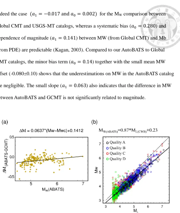
AutoBATS and BATS catalogs... 40 Figure 2.8 MW differences between AutoBATS and Global CMT catalog and relation
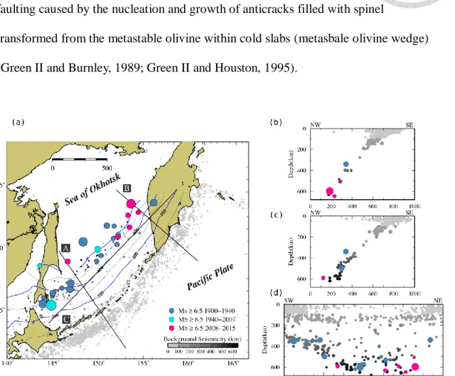
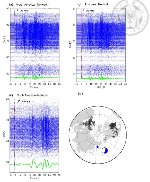
of MW(ABATS) and ML(CWB). ... 42 Figure 2.9 Cross-sections of focal mechanisms from AutoBATS catalog. ... 46 Figure 3.1 Historical deep-focus seismicity of Kuril subduction zone since 1900. ... 51 Figure 3.2 Coherently aligned vertical seismograms and seismic networks used for BP
images. ... 59 Figure 3.3 High frequency P-wave (0.5~2.0 Hz) 3D BP imaging snapshots for the
mainshock. ... 61 Figure 3.4 Low frequency (0.125~1.0 Hz) 3D BP imaging snapshots for mainshock. .. 64 Figure 3.5 3D BP imaging results summaries for the mainshock. ... 65 Figure 3.6 Coherently aligned vertical seismograms of two aftershocks from EU
seismic network. ... 67 Figure 3.7 High frequency P-wave 3D BP images of two aftershocks by using EU
array data. ... 67 Figure 3.8 Synthetic tests of vertical rupture scenarios. ... 70
Figure 3.9 Synthetic tests of SE-ward dipping rupture scenario. ... 72 Figure 3.10 Synthetic tests of two-stage anti-parallel rupture scenarios. ... 73 Figure 3.11 The tectonic setting of northern Kuril subduction zone and the BP imaging
results of 2013 great Okhotsk deep earthquake sequence, including the mainshock and two largest aftershocks... 77 Figure 3.12 Cross-sections of the 3D BP results of 2013 Okhotsk mainshock. ... 78 Figure 3.13 Cross-sections of the 3D BP results of two aftershocks. ... 81 Figure 4.1 Tectonic settings of Meinong earthquake and the profiles showing BP
results and aftershock distributions. ... 87 Figure 4.2 The resulting BP images from the AU and EU seismic array. ... 93 Figure 4.3 Teleseismic waveforms, travel time differences between depth phases and P
arrivals and the amplitude ratio of pP/sP... 94 Figure 4.4 Directivity analysis result, the rupture distances and times at EU and AU
array and the comparison of BP result with finite fault inversion. ... 97 Figure 5.1 Map showing seismicity and tectonic settings in Taiwan ... 104 Figure 5.2 The resulting BP images of 2010 Jiashian earthquake from the EU and AU
seismic array. ... 111 Figure 5.3 The resulting BP images of Jiashian and Meinong earthquakes. ... 113 Figure 5.4 Global displacement waveforms of 2010 Jiashian earthquake. ... 117 Figure 5.5 The directivity analysis results and comparison with BP results for 2010
Jiashian earthquake. ... 118 Figure 5.6 Fault settings for 2010 Jiashian and 2016 Meinong doublet events. ... 122 Figure 5.7 Earthquake numbers and temporal b-value variation in JSMN fault and
Southwestern Taiwan. ... 125 Figure 5.8 3D sketch of fault geometry settings and the Coulomb stress change induced
by Jiashian and Meinong doublet. ... 129
Figure A1. The epicenter and array distribution and the aligned vertical velocity
waveforms of two arrays. ... 132 Figure A2. Synthetic velocity seismograms on the vertical component compared with
the observed ones shown in Fig. 3(a). ... 133 Figure A3 The P-wave ray paths, 1D average velocity model and the tomographic
images along the ray path... 134 Figure A4 Test for recovery of a synthetic source scenario by the MUSIC BP method.135
Figure B1 The seismic arrays and aligned P waves used for the BP images of 2010 Jiashian earthquake. ... 138 Figure B2 Synthetic velocity seismograms for comparison with the observed ones
shown in Figure 5.4 ... 139 Figure B3 1D average velocity models and tomographic images along the ray paths of
P and depth phases. ... 140 Figure B4 The stress inversion results. ... 141 Figure B5 The earthquake numbers and temporal b-value variation. ... 142 Figure B6 The 3D sketch of two causative faults for Jiashian and Meinong doublets
and the Coulomb stress change induced by two earthquakes. ... 143 Figure B7 The 3D sketch of JSMN fault or two-separated faults and the Coulomb
stress change across the SCM and TN fault areas induced by 2010 Jiashian earthquake. ... 144
List of Tables
Table 2.1 Quality classifications of the misfit and non-DC component in the released AutoBATS MT catalog ... 27
Chapter 1 Introduction
One of the key problems in seismology is the understanding of earthquake source processes. The kinematic source properties of an earthquake include the seismic moment, fault geometry, dislocation across the fault plane and the spatio-temporal distributions of the slip. When an earthquake occurred, besides the origin time and hypocenter location, the fundamental information of focal mechanism describing the fault geometry and dislocation across the fault plane is directly related to the response of the tectonic stress accumulation and release at the fault zone. Other than the focal mechanism, the rupture parameters including the rupture extent, speed, direction, duration and stress drop would control the behavior of the rupture front and reveal the physical properties of the fault itself. The estimated seismic moment and kinematic source rupture characteristics are the basis for further simulations of dynamic rupture scenario of an earthquake.
Understanding of the lithospheric deformation and tectonic stress regimes relies on continuous long-term observations of seismicity accompanied with a complete and reliable focal mechanism catalog. Routine determinations of focal mechanisms of global earthquakes with moment magnitude Mw5.5 or regional earthquakes in seismically vulnerable areas had been developed and performed by many state
agencies or research institutes, such as Global Centroid Moment Tensor (Global CMT) project (Ekström et al., 2012), the United States Geological Survey (Spikin, 1986), GEOFON (Bormann, 2012), and GEOSCOPE (Vallée et al., 2011). In general, the earthquake focal mechanism can be represented by 5 or 6 independent components of the moment tensor (MT) associated with equivalent body-force couples acting on the
point-source location. Then the moment tensor solution of an earthquake can be simply obtained by a linear inversion of the observed waveform data and theoretical Green’s functions. However, the challenges of retrieving stable and reliable moment tensor solutions reside in the intrinsic noises, imperfect coverage of data and inaccuracy of the Green’s functions because of an inappropriate velocity model and mislocated centroid position used. In recent years, owing to the speedy progress of the computational capacities and data transmission of seismic networks, the real-time moment tensor inversion becomes possible to quickly gain the basic earthquake information for characterizing and responding to potential seismic hazards. Lee et al.
(2014) developed a real-time moment tensor monitoring system (RMT) to
automatically detect and simultaneously determine the epicenters and moment tensors of earthquakes in Taiwan, achieved at the expense of enormous computational
resources. On the other hand, studies of seismogenic structures and seismotectonics demand a complete earthquake catalog that contains reliable and well-resolved
moment tensor solutions. It is thus necessary to carry out a comprehensive exploration of several inversion settings, including the data, centroid location, velocity structure, and others that could lead to unstable or ambiguous inversion results but often were neglected in real-time solutions.
In the first part of my PhD thesis, I focus on establishing a new AutoBATS moment tensor inversion algorithm mainly for abundant regional seismicity in Taiwan.
The goal of the study is to report both near real-time and stable MTs by taking into account the uncertainties of the inversion settings mentioned previously. Different from Lee et al. (2014) conducting a grid search of candidate earthquake locations using continuous longer-period broadband seismic data at a few BATS stations, I prefer to
take the best use of high-precision hypocenters to lower the mislocation effects on the MT solutions, which are determined by much denser CWBSN (Central Weather Bureau Seismograph Network). Instead of fixing the inversion settings for all the earthquakes that occurred in tectonically distinct settings, I would like to deliver the final moment tensor solutions together with the validation of the stability or reliability of the solutions by scanning four different Moho-depth models representative of the structures in the Taiwan region, three strategies of data selection, and three filtering frequency bands for all the used data.
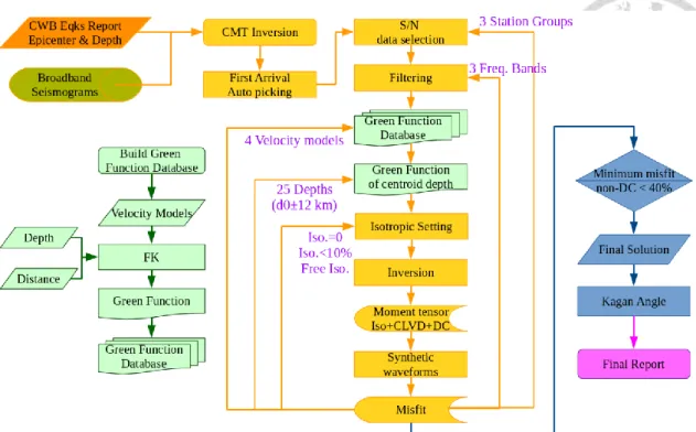
In Chapter 2 , I present the new AutoBATS moment tensor inversion approach and its application to regional earthquakes in the Taiwan area. The reliability of the inversion scheme is verified by making the comparison of our newly obtained CMT catalog with the Global CMT solutions and the previous BATS catalog. Benefiting from this fast, reliable inversion scheme, I also update the regional moment tensor catalog for Taiwan earthquakes from 1996 to 2016. A new relation between moment magnitude (MW) and local magnitude (ML) is also examined based on our complete AutoBATS MT catalog. Figure 1.1 illustrates the flow chart of the newly developed AutoBATS moment tensor inversion method which has already been implemented in the real-time moment tensor report system of Data Management Center of IES (DMC-IES).
Figure 1.1 Flowchart of new real-time AutoBATS MT inversion scheme.
In general, a point-source approximation for major and great earthquakes is not sufficient to characterize the earthquake rupture propagating away on the finite-size fault plane. Therefore, the second part of the thesis is devoted to investigate the rupture characteristics of large earthquakes using high-density, high-frequency seismic array data.
Over the past several decades, numerous studies have employed different waveform inversion methods such as the multiple point source moment tensor
inversion (Kao et al., 2000; Chen and Wen, 2015) and finite fault inversion (Antolik et al., 1996; Ji et al., 2002; Ye et al., 2012) to unravel the complex rupture history of many devastating earthquakes. These methods intend to recover the details of the rupture process by modeling a finite earthquake source as multiple subevents or discretized subfaults on the fault plane with variable source parameters. Although the
forward modelling theory that forms the foundation for the source inversion and the numerical inversion algorithm have been developed for years and become routinely applied to global large earthquakes, the finite-source inversion is known to be a notoriously ill-posed and underdetermined geophysical inverse problem (Ide, 2015) with too many unknown, poorly constrained model parameters involved in the
inversion. As a result, it leads to highly non-unique results that strongly depend on the imposed a priori constraints such as the fault geometry, rupture speed, rise time, and etc. In addition, the relative complexity of high-frequency seismograms often affected by strong crustal velocity heterogeneity but not accounted properly in the waveform inversion limits the use of shorter period waveform data in the inversion.
Contributed by the worldwide deployment of dense seismic arrays such as USArray, ORFEUS (European network) and Hi-net (Japanese network), a high-resolution back projection (BP) technique alternative to the finite source waveform inversion have been widely applied to imaging the rupture propagation history of large earthquakes. In contrast to the inversion approach, the BP method requires neither the adjustment of a priori damping and smoothing parameters imposed on the inversion models nor the knowledge of the Green’s functions, fault geometry, and rupture kinematics. It basically retrieves and stack coherent, high-frequency teleseismic seismic wavefield recorded across the array and project them back in time to track the positions of the strongest energy radiators among subfault grids throughout the rupture duration. As the onsets of the wavetrains used in the BP imaging are
aligned properly, the errors in predicted travel times due to the heterogeneous velocity structure between the source and receiver are negligible. Ishii et al. (2005) first
demonstrated the efficacy of the BP method to image a ~1300-km long rupture
propagating northward for the 2004 Sumatra-Andaman megathrust earthquake. Since then, it has become an effective approach to illuminate the rupture process for major earthquakes, such as the 2008 Sichuan earthquake, 2010 Chilean earthquake, and intermediate- and deep-focus earthquakes (Xu et al., 2009; Kiser et al., 2011b; Kiser and Ishii, 2012; Koper et al., 2012).
The classical BP approach, similar to the time-domain beamforming technique, shifts the traveltime moveout from a trial subfault grid relative to the hypocenter and stacks the moveout-corrected waveforms across the array to locate the energy radiation point associated with the maximum amplitude of the stacked waveforms integrated over certain time intervals. However, Ishii et al. (2007) noticed the spatial and temporal artifacts of the ghost stacks from the synthetic BP experiments that could cause the biased estimate of the time and location of the energy radiators. Such the ghost swimming artifact mainly arises from nonstationary seismic wavetrains within which the amplitudes are highly variable such that the weak arrivals in the beamforming image can be obscured by the movement of large-amplitude arrivals (Walker and Shearer, 2009; Xu et al., 2009; Meng et al., 2012a, 2012b). Meng et al. (2012b) developed a more viable BP method for non-stationary seismic waveforms based on the subspace-based method, the Multiple Signal Classification (MUSIC) algorithm. It has been demonstrated that the MUSIC BP technique provides superior resolution of the source images compared to that obtained with the classical time-domain BP method by adopting the “reference window” strategy to mitigate the artificial
swimming effect efficaciously. Despite of the improvement of the BP method, it is still difficult to entirely suppress the smearing effect as illustrated in Figure 1.2b because of the intrinsic trade-off between travel time and distance. Therefore, most of the BP
imaging studies is restricted to 2D applications only, i.e. the candidate radiation sources confined in an assumed horizontal plane positioned at the focal depth of the earthquake.
On May 24, 2013, the largest deep earthquake ever recorded by modern seismic networks struck about 609 km beneath the Sea of Okhotsk. The focal mechanism from the Global CMT solution indicates this deep earthquake ruptured on either a
sub-horizontal or sub-vertical fault plane. The finite-fault inversion reaches the inconclusive fault-plane orientation because the results of assuming either one of the nodal planes yield equal fits to the observed and synthetic waveforms (Ye et al., 2013).
On the other hand, Chen et al. (2014) and Zhan et al. (2014) performed the multiple point source inversion and directivity analysis but obtained opposite conclusions on the actual fault plane. In Chapter 3 , I attempt to develop a three-dimensional (3D) MUSIC BP method (Figure 1.2a) to resolve the ambiguity between the sub-vertical and
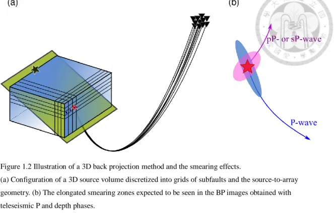
sub-horizontal fault plane. To facilitate suppressing the smearing effects in the BP image and retrieve the stable rupture propagating process in 3D, I include the 3D BP images obtained by depth phases, pP, which travel upward to the surface and turning back to the distant stations and have the take-off angle different from the down-going direct P-wave. Since the smearing zone is parallel to the ray path from the source to the receiver array, combining the BP images obtained with different phases would help reduce the smearing area (Figure 1.2b).
Figure 1.2 Illustration of a 3D back projection method and the smearing effects.
(a) Configuration of a 3D source volume discretized into grids of subfaults and the source-to-array geometry. (b) The elongated smearing zones expected to be seen in the BP images obtained with teleseismic P and depth phases.
The combined P- and pP- wave 3D BP image of the 2013 Okhotsk earthquake seen from the North American (NA) seismic network shows a two-stage, anti-parallel rupture. The rupture propagates about 30-40 km northeastward during the first stage; it then jumps to greater depths and propagate at least 80 km in the reverse (S-ward) direction. The two anti-parallel ruptures are separated by a vertical distance of about 10-15 km. The average rupture speeds during the two stages are 3.0-3.3 and 4.25-4.80 km/s, respectively. The initial NE-ward rupture ends near the northern tip of the
subducted Pacific slab that most likely has been heated up by the ambient warm mantle and asthenospheric flow around the slab edge (Peyton et al., 2001; Park et al., 2002;
Davaille and Lees, 2004a). This may cause a relatively slower speed of the first NE-ward propagating rupture as well as prevent it from continuously growing.
In order to understand the resolution and limitations of the 3D MUSIC BP
technique, I perform a suite of synthetic experiments that mimic several possible rupture scenarios for the Okhotsk earthquake, including the rupture propagating vertically up- or down-ward, and horizontally perpendicular or parallel to the source-to-array azimuth. All of these synthetic results show the capability of the 3D P-wave BP MUSIC method to recover the hypothetical subevents. As expected, the combined P- and pP-waves BP images can help stabilize the resolved rupture image and locate the energy radiators with much smaller spatial uncertainties than that obtained with P waves only.
As the BP method mainly uses high-frequency teleseismic wavefield for source imaging, there are few applications to shallow earthquakes with magnitude less than 7 that could also produce destructive hazards. There are on average one to three
earthquakes with magnitude greater than 6 that hit the Taiwan region every year, and some of them have caused severe damages and fatalities such as the 2016 Meinong earthquake and 2018 Hualian earthquake. To better understand the rupture kinematics of these earthquakes and corresponding seismogenic fault zones, I applied the MUSIC BP imaging and directivity analysis to unravel the rupture process of two strong earthquakes, the 2016 Meinong and 2010 Jiashian earthquakes that recently occurred nearby in southern Taiwan with comparable magnitudes and focal mechanisms.
In Chapter 4, I present the first application of the MUSIC BP method to quantify the details of the rupture process for a moderate earthquake, the 2016 Mw 6.4 Meinong earthquake that severely hit southwestern Taiwan, a region with relatively low
seismicity in the past and caused the deaths of over 100 people in the populated Tainan city about 30 km west of the epicenter. I use high-frequency P and depth-phase sP wavetrains from the dense European (EU) and Australian (AU) seismic networks. The
P-wave BP results either from the EU or AU array show a consistent NW-ward rupture extending about 16 km with a single-peak radiation burst and duration of ~7 s. Besides, through forward waveform modeling, the slowness-backazimuth analysis, and
radiation pattern of depth-phase sP/pP amplitude ratios, I confirm the second displacement pulse that begins ~8 s after the onset of the first P-wave pulse mainly consists of the depth-phase pP and sP energy. Therefore, I conduct the same BP imaging using the aligned sP wavetrains. The integrated P- and sP-wave BP images resulting from the EU and AU array data are overall in accordance with each other showing a unilateral subhorizontal rupture propagating northwest. To verify the
kinematic rupture properties derived from the BP imaging, I also employ the directivity analysis assuming a kinematic unilateral rupture model using global broadband
displacement waveforms.
As demonstrated by the study of the Meinong earthquake, the MUSIC BP
technique has shown great success in unraveling the rupture behavior of moderate-size earthquakes generally with relatively short rupture length about tens of kilometers and source duration about a few seconds. Therefore, I attempt to apply the same approach to studying the rupture process of the 2010 Jiashian earthquake which shares several seismological similarities with the 2016 Meinong earthquake, including the nearby epicenter, similar focal mechanism and comparable seismic moment. The results are summarized in Chapter 5.
According to the integrated P- and sP-wave BP images obtained with the EU and AU array data, I found the Jiashian earthquake predominantly ruptured toward
northwest as the Meinong earthquake did. However, unlike the Meinong event with a nearly horizontal rupture, the Jiashian earthquake ruptured obliquely in both the
along-strike and updip direction, which is about 16-20° from the horizontal plane. The estimated rupture length and duration is about 10-11 km and 4-5 s, respectively, which give the average rupture speed similar to that of the Meinong earthquake. Similarly, I conduct the directivity analysis to validate our BP results. I perform a grid search in the space of the rupture length and velocity, and the strike and dip of the rupture
propagation direction and find the optimal solution that yields a global minimum misfit of observed and predicted apparent rupture durations. The F-test shows that the
additional testing variables, the rupture strike and dip, are statistically significant to improve the fit between the observed and predicted source time duration.
Motivated by the similarity of the seismic moment tensor and rupture properties between the Jiashian and Meinong earthquake as well as the spatial distributions of the mainshock and aftershock sequences, I proposed a blind subsurface fault striking NW and dipping to NE (hereafter referred as to the JSMN fault) is the causative fault responsible for the occurrence of the two earthquakes. Besides, I investigate the temporal b-value variations and static stress changes induced by the two events. By compiling all the observations and analyzing results, I propose the Jiashian and Meinong earthquakes are the doublet events which have occurred as a result of failure of the two strong asperities on the JSMN fault. After continuous stress buildup on the fault for at least 45 years mainly exerted by the plate convergence, the accumulated stress exceeding the strength of the smaller asperity on the deeper eastern end of the fault released and initiated the rupture of the Jianshian earthquake. The static Coulomb stress transfer triggered by the slip of the Jianshian event suggests an additional stress increase in the vicinity of the shallower western asperity. With additional tectonic stress loading for six years, the failure of the shallower and stronger asperity took place
and initiated the rupture of the Meinong earthquake.
Chapter 2 A new automatic full-waveform regional moment tensor inversion algorithm and its applications in the Taiwan Area
Original published in Jian, P.-R., T.-L. Tseng, W.-T. Liang, and P.-H. Huang (2018). A New Automatic Full-Waveform Regional Moment Tensor Inversion Algorithm and Its Applications in the Taiwan Area, Bull. Seismol. Soc. Am.
2.1 Abstract
A new algorithm is developed in this study to automatically determine regional moment tensor (MT) and its centroid depth with real-time waveforms in 2-4 minutes after the Central Weather Bureau (CWB) issues an earthquake notice. The program selects 3-7 BATS (Broadband Array for Taiwan Seismology) stations under three
criteria: best azimuthal distribution, highest signal-to-noise ratio, and shortest distances.
It then inverts MT solutions in parallel with various settings including Moho depth of velocity models, frequency bands, and isotropic constraints. The optimal solution is determined by searching for the best waveform-fit with an acceptable
non-double-couple component from the results of combinations of these inversion settings. Our new rapid MT report system greatly reduces computational resources and avoids human judgments. By applying this full-scanning approach on BATS (named AutoBATS), we re-determine the MTs for over 3000 regional earthquakes from 1996 to 2016 to provide the most up-to-date MT catalog for the Taiwan area. The AutoBATS MTs are overall consistent with the Global Centroid Moment Tensors with a mean difference in Kagan angle of 22.0±16.6° and MW of -0.08±0.10. Those focal mechanisms better illuminate the tectonic structures owing to the much improved
resolving ability for shallow (<10 km) and deep (>140 km) earthquakes. With the new regional MT catalog, we refine the relationship between moment and local magnitudes:
MW = 0.87 ML+0.23 for the Taiwan region.
2.2 Introduction
Fast determination of source parameters of regional large earthquakes are crucial for government agencies to properly and quickly respond to cases of serious seismic hazards. Reliable estimates of the seismic moment and focal mechanism are
particularly important because these two parameters are directly related to the extent and severity of the seismic damage caused by earthquakes. For long-term evaluation of the seismic hazard of seismically active regions, a robust regional moment tensor catalog is the most fundamental information for advanced studies like regional
tectonics, strain-stress monitoring of the lithosphere, and strong motion simulation for hazard evaluations.
For moderate-to-large earthquakes with MW above ~5.5 worldwide, moment tensor (MT) solutions are available freely from agencies/organizations such as the Global Centroid Moment Tensor (CMT) project (Ekström et al., 2012), the United States Geological Survey (Spikin, 1986), GEOFON (Bormann, 2012), and
GEOSCOPE (Vallée et al., 2011). In theory, both the centroid moment tensor (CMT) and point source parameters (centroid position and origin time) are determined by inverting very long-period seismic waveforms recorded at tele-seismic distances (Dziewonski et al., 1981). Over the past two decades, regional MT inversion has also
become a routine process to release MT or CMT local catalogs for small-to-moderate earthquakes since regional seismic networks have built up in many seismically active areas (Dreger and Helmberger, 1993; Sileny et al., 1996; Kao et al., 1998a; Fukuyama and Dreger, 2000; Braunmiller et al., 2002; Kubo et al., 2002; Pondrelli et al., 2002;
Stich et al., 2003; Bernardi et al., 2004; Ito et al., 2006; Cambaz and Mutlu, 2016).
With increasingly dense regional networks developing worldwide, near real-time automatic MT inversion systems are becoming possible due to the large improvements in data transmission and computational capability in the last decade (Bernardi et al., 2004; Rueda and Mezcua, 2005; Ito et al., 2006; Nakano et al., 2008; Scognamiglio et al., 2009; Lee et al., 2011). On a regional scale, genuine CMT solutions can be inverted based on local long-period waveforms with the centroid position often obtained by grid-search approaches (Ito et al., 2006; Lee et al., 2014).
Taiwan, an extremely seismically active area in the western Pacific, was one of the earliest countries to have a regional MT reporting system. Kao et al. (1998a) established the moment tensor inversion algorithm using long-period waveforms recorded by the local network BATS (Broadband Array in Taiwan for Seismology operating under the Institute of Earth Sciences (IES) of Academia Sinica, Taiwan.
Since 1995, the Data Management Center of IES has routinely inverted and published over 2000 moment tensor solutions for regional earthquakes with ML above 4.0. The MTs released by IES BATS (so-called BATS CMT) have been widely adopted by research communities for further investigations in the Taiwan area on earthquake rupture characteristics (Huang et al., 2008; Lee et al., 2008), seismotectonic studies (Kao et al., 1998a; Kao and Jian, 1999, 2001; Kao and Chen, 2000; Lallemand et al., 2001; Angelier et al., 2009; Chen et al., 2009; Huang and Lin, 2017), seismic moment
magnitudes, and seismic hazard evaluations e.g., (Chen et al., 2008).
To achieve fast estimates of MTs for Taiwan earthquakes, IES BATS currently performs moment tensor inversion with a set of fixed parameters after receiving alarms issued by the Central Weather Bureau (CWB) of Taiwan. However, data selection and quality examination on inversion results are still performed manually. Usually, the MT reports can be provided within a few hours. From a different perspective, Lee et al.
(2014) developed a real-time MT system that reports the centroid hypocenter location with a 10-km spatial resolution and the corresponding MT within 2 minutes by calculating MTs of a continuous data stream recurrently recorded by a fixed subset of BATS stations. The drawback is that this state-of-the-art system requires significant computational resources to approach a truly real-time solution that is independent of the CWB report.
No matter which frameworks are chosen, it is unquestionable that the reliability of the MT solution requires the inversion itself to be performed with suitable parameters and settings. In particular, lateral changes in velocity structure are apparent in Taiwan e.g. (Rau and Wu, 1995; Huang et al., 2014), and a fixed one-dimensional (1D) model cannot be perfect for each event analyzed. The MT solutions may be improved by adjusting 1D velocity models for each event-station pair, selecting alternative stations, and trying different frequency bands for each station. In the past, for BATS MT, further fine-tuning was also manually processed (Kao et al., 2002; Liang et al., 2004).
However, this traditional approach is too tedious and inefficient to satisfy current demand, leading to the desire for a compromise. In addition, it is important to explore how large the variances can be if the solutions are inverted with different parameters or settings.
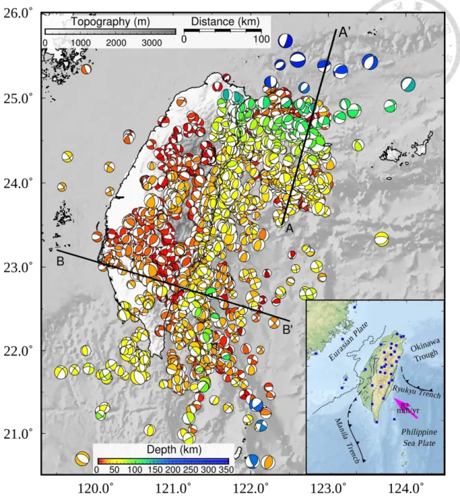
Figure 2.1 AutoBATS MT solutions for earthquakes from May 1996 to April 2016.
The beach ball colors represent the centroid depth determined by MT inversion. The beach ball size is scaled with the moment magnitude. The lower right inset shows the tectonic setting in the Taiwan area.
The pink thick arrow indicates the direction of the converging Philippine Sea plate relative to the Eurasian plate. BATS broadband stations are denoted by blue squares (excluding stations in the South China Sea). The dotted line delineates the 2000 m isopach of Cenozoic sediments.
In Taiwan, reporting MT solutions while satisfying both fast and reliable obligations is a great challenge due to strong heterogeneity in velocity structures, possible mislocation of off-island earthquakes, and unavoidable long-period
background noises for those stations located close to shore or on small islands. In this study, we develop a new automatic approach to achieve the goal of retrieving highly reliable regional MT solutions in near real-time for small-to-moderate earthquakes in Taiwan. We are not attempting to fully determine the centroid hypocenters. Instead, we take advantage of the overall efficiently and precisely determined epicenter origins from CWB. Therefore, only the centroid depth and MT of the events are constrained in our MT report. To reduce the manual efforts on searching suitable inversion settings for each earthquake, we determine the final MT solution among the inversion results by systematically exploring various key settings or parameters, including different frequency bands, station-selection strategies, and 1D velocity models. Then, we can demonstrate the variability of the solutions and discuss which factors are more
influential on the MTs for each event. Finally, we provide 20 years of well-determined focal mechanisms for the Taiwan region that exhibit details of tectonic features.
2.3 Moment tensor inversion and regional waveform data
Linear moment tensor inversion is based upon the representation theorems in which the observed displacement waveforms are the combined effects of the earthquake source and Green’s functions (Aki and Richards, 1980). In principle, Green’s functions contain propagation effects in a layered Earth’s structure from
earthquake to station, whereas a moment tensor, a matrix of 6 independent elements, gives the equivalent radiation of faulting on a point source. In the case of zero-volume change, the third isotropic element is compensated by the sum of the other two on the diagonal of the matrix (Jost and Herrmann, 1989), leading to five independent
variables to solve. With a properly derived velocity model and quality waveforms, the moment tensor can be directly inverted by minimizing the overall differences between the observed and simulated three-component waveforms in a least squares sense (Stump and Johnson, 1977). The fault parameters are then derived from the double-couple (DC) component of the moment tensor.
In the current CMT inversion algorithm of BATS, Kao et al. (1998a) used a reflectivity-based method of Yao and Harkrider (1983) to calculate Green’s functions.
In this study, we employ the frequency-wavenumber integration technique as an alternative which is capable of calculating both static and dynamic surface
displacement (Zhu and Rivera, 2002). For the goodness of waveform fitting in the inversion, we principally follow the definition of a cross-correlated,
similarity-sensitive misfit function (introduced by (Mellman et al., 1975; Kao et al., 1998a), which emphasizes the coherence between the observed and synthetic waveforms more than the absolute amplitudes (Wallace et al., 1981). To further
account for the differences in relative amplitude, we adopt the misfit equation for each component as follows: 𝐸 = 1 −min (𝑓𝑖(𝑡)𝑚𝑎𝑥,𝑔𝑖(𝑡)𝑚𝑎𝑥)
max (𝑓𝑖(𝑡)𝑚𝑎𝑥,𝑔𝑖(𝑡)𝑚𝑎𝑥)
∫ 𝑓𝑖(𝑡)∗𝑔𝑖(𝑡)𝑑𝑡
√∫ 𝑓𝑖(𝑡)2𝑑𝑡 ∫ 𝑔𝑖(𝑡)2𝑑𝑡, where fi(t) and gi(t) are observed and synthetic waveforms in displacement, respectively; fi(t)max and gi(t)max are the maximum amplitude of observation and synthetic waveforms,
respectively (Kao and Jian, 1999; Huang et al., 2017).
In this study, all broadband waveforms come from BATS, a local network
currently consisting of a total of 36 broadband stations in the Taiwan area (Figure 2.1, inset) who have provided high-quality continuous seismic data since 1996 (Institute of Earth Sciences, Academia Sinica, Taiwan, 1996). The initial information of
earthquakes, including epicenter, focal depth, and origin time, are taken from CWB. To reduce the effects of mislocation errors on inversion results, we only use
well-determined hypocenters of earthquakes that are verified manually with the quality-checked data by CWB. The centroid depth of the MT solution is estimated together with the MT inversion by a grid-search approach as in many CMT studies (Dreger and Helmberger, 1993; Zhu and Helmberger, 1996), as well as the previous BATS inversion (Kao et al., 1998a). Here, we perform MT inversion at a 1 km interval for a depth range ± 12 km with respect to the initial focal depth, and the centroid depth is determined from the smallest misfit among the 25 solutions.
Although the moment tensor inversion itself is a linearized problem through Green’s functions and seismic displacement waveforms, non-uniqueness or large variances of inversion results are common because of non-linear effects/bias from the different 1D velocity model assumptions for Green’s functions, the frequency band used for data processing, and the method of selecting stations. Therefore, our approach is to retrieve stable MT solutions by systematically scanning the solutions from all combinations of station-choosing strategies, varied velocity models, and different frequency bands. The scanning parameters and setting criteria are introduced in the next section.
2.4 Automatic determination of the optimal MT solution with thoroughly scanned parameters
To efficiently achieve stable and reliable results for moment tensor inversion, the first important and necessary step is to avoid manual data selection before the
inversion. In this study, we only consider stations whose average signal-to-noise (S/N) ratios of three-component waveforms are greater than 2.0 in the desired frequency band (0.01~0.09 Hz). We take 150 s time windows before and after the P arrival to estimate the spectra and calculate average point-by-point S/N with 5-point moving time-window smoothing. We exclude stations with epicentral distances smaller than 30 km to reduce the mislocation effect. Since many studies typically use three or more three-component broadband stations for regional moment tensor inversion (Dreger and Helmberger, 1993; Zhu and Helmberger, 1996; Kubo et al., 2002; Pondrelli et al., 2002;
Rueda and Mezcua, 2005; Clinton et al., 2006; Ristau, 2008), we selected a minimum of 3 to a maximum of 7 S/N-qualified stations to start the inversion based on three different criteria: (1) the best azimuthal coverage, (2) the highest S/N, and (3) the shortest epicentral distances. For earthquakes inside a homogeneous network, the most logical and easiest approach for criterion (1) is to divide stations evenly into 8 half quadrants according to azimuth and pick at least one S/N-qualified station in each sector. Unfortunately, this simple method is not appropriate for Taiwan due to restricted azimuthal coverage in most cases since the majority of earthquakes occur near the coast and eastern offshore region. To accommodate this natural condition, we retain the stations at the minimum and maximum azimuth, and use these two azimuths as boundaries to divide the remaining stations into three even sectors. We then pick one
to three stations randomly in each sector so that criterion (1) is fulfilled. For criteria (2) and (3), stations are chosen according solely to their mean S/N and epicentral
distances.
It is normally expected that better azimuthal coverage improves reliability of MT solutions. The problem of selecting stations solely based on azimuthal coverage in the Taiwan area is that the selected stations near the coast or on small islands are
occasionally contaminated by long-period ambient noises even though the average S/N might be slightly better than threshold value. Criteria (2) and (3) not only provide other possible choices of stations, but the consistencies among resulting solutions can further ensure the MT solutions are insignificantly biased by those stations with notable noises near the shore or at far distances. Note that the quality (S/N) of regional waveforms is usually site-dependent and unrelated to epicentral distances; therefore, the three different criteria are complementary.
Once stations are selected, we perform the inversions with different parameter settings. To accommodate the velocity variations in the Taiwan region and to improve the stability of inversion with the longest possible periods, we apply three different frequency bands and four velocity models for all selected stations in the inversions. For each earthquake, three consecutive passbands are applied from the followings 5
standard frequency ranges: 0.01~0.04 Hz (25~100 s), 0.02~0.06 Hz (16~50 s), 0.03~0.08 Hz (12~33 s), 0.04~0.09 Hz (10~25 s), and 0.05~0.15 Hz (7~20 s). The choice depends on the local magnitude reported by CWB. For earthquakes with a local magnitude above 5, within 3.5 to 5, and below 3.5, the lowest corner frequency starts from 0.01, 0.02, and 0.03 Hz, respectively.
For the velocity models, it is unrealistic to create a high-resolution 1D velocity
model which reflects all the path effects for each event-station pair because the seismic waves usually travel through distinct structures in Taiwan (especially along the
east-west direction). Considering the waveforms for MT inversion have been filtered for relatively long periods, we start with a simple three-layer model averaged from a 3D tomography model of Taiwan (Rau and Wu, 1995) as a reference. This model, with Moho depth set at 40 km, has been used for 20 years by the current BATS MT
inversion, and simulations in waveforms are reasonably good (Kao et al., 1998a, 2002;
Kao and Jian, 1999; Kao and Chen, 2000; Liang et al., 2004). We then further consider the effect of regional variations of Moho depths from 20 to 50 km under different geologic units that were revealed by receiver-function and tomography studies (Wang et al., 2010; Kuo-Chen et al., 2012; Huang et al., 2014). Since the dominant periods used are more sensitive to structure deeper than 20 km relative to the shallow crust within 10 km (Dahlen and Tromp, 1998), we create a series of velocity models by changing the Moho at 5 different depths ranging from 25 to 45 km with intervals of 5 km. Each candidate potentially represents the average/pseudo structure under the paths covered by the event. Moho depths between 30 and 45 km are used for inland
earthquakes, while a shallower range from 25 to 40 km is considered for offshore cases.
After carefully examining the inversion results, we confirmed that trying different Moho-depth models can effectively reduce misfit and the compensated linear vector dipole (CLVD) component. Following Dreger (2003), we allow Green’s functions to shift by ±2 seconds for each station to lower the misfit due to the possible mislocation and the imperfectness of the velocity model. For fast moment tensor inversion, the Green’s functions of each 1D model are pre-calculated and stored in the databases with a 1 km grid size in distance and focal depth.
For a more realistic simulation of synthetic waveforms, we assign 0.5, 1.0, and 2.0 seconds as duration of source time function for earthquakes with magnitude smaller than 4, between 4 and 6, and above 6, respectively. Since events associated with volcanic activities have been reported in the Okinawa Trough in northeast Taiwan (Lin et al., 2007), our newly developed MT inversion method includes three different isotropic conditions: free-constrained, limited (≤10%), and zero isotropic components.
For the free-constrained or zero isotropic component, we simply invert either 6 or 5 independent elements of the moment tensor. For limited isotropic constrained inversion, we compose a weighting vector inside the kernel matrix, in which the sum of three isotropic elements equals 0, as shown in following
form: [𝑑
0] = (𝑤 𝑤 𝑤 0 0 0𝐺 )(𝑚11 𝑚22 𝑚33 ⋯)𝑇. The inversion is performed iteratively with an initial weighting factor (w) 1, and then adjusted by increments of 1 until the isotropic component of the moment tensor is reduced to 10% or lower.
The AutoBATS MT inversion starts with auto picking of the first P arrivals for each station (Allen, 1978). The system then performs all inversion processes
concurrently with different combinations of settings/parameters mentioned above using the GNU parallel tool (Tange, 2011). Among those inversion results, the one with the minimum misfit and applicable non-double-couple (non-DC) component is reported as the final/preferred MT solution (see Table 2.1 for classifications). Generally, we expect both the CLVD and isotropic components of the tensor to be low for small- to
moderate-size tectonic earthquakes associated with shear faulting and relatively
uncomplicated ruptures. According to Kagan (2002), an additional non-DC component can be introduced due to the data contamination of background noises, an over
simplified velocity model, or the mislocation of earthquakes; therefore, we set up rigorous criteria for non-DC. Only solutions with an isotropic component 20%, CLVD 30%, and non-DC40% are accepted for reporting. For each resultant MT solution, we assign a quality factor (QF) according to the waveform misfit and non-DC component (Table 1). Although the MT solutions with limited non-DC components were reported, the AutoBATS parameter-scanning algorithm is capable of searching for the non-tectonic seismic events if the non-DC criterion is removed.
In this study, we applied the procedure of AutoBATS MT inversion to determine a total of 3058 solutions for earthquakes with a ML greater than 3.5 between May 1996 and April 2016 in the Taiwan region (Figure 2.1). Figure 2.2 and Figure 2.3 demonstrate how well the focal mechanisms are constrained by the AutoBATS
inversion for a shallow earthquake (ML=4.9) inland and another intermediate-depth event (ML =6.7) offshore, respectively. In each event, the best solution of focal mechanism and the corresponding stations used are highlighted (Figure 2.2a, and Figure 2.3a). Inversion results from different combined settings (such as Moho depth of models, frequency bands, and centroid depths) are directly compared in terms of their misfits and non-DC components. For the 2015/05/25 inland earthquake, the distribution of misfit and non-DC contours shows that filtering at a lower frequency band (0.02~0.06 Hz) and a model with a deeper Moho of 40 km yields the smallest misfit for this normal faulting event with a centroid depth of 10 km (Figure 2.2b). Most inverted tensors are close to pure normal-faulting as indicated by the triangle diagram of focal mechanism (Figure 2.2d). The triangle diagram, developed by Frohlich (2001), is an effective way to demonstrate the fault-type partitioning and the frequency
distribution of the focal mechanisms from the inversion results of all tested parameters.
Figure 2.2e further gives the distribution of the Kagan angles (Kagan, 2003), K-angle hereafter, the smallest 3D rotation angle measured between the best focal mechanism and other solutions. It can be shown that the differences between solutions are more sensitive to the focal depths than the frequency band or velocity model for this earthquake. The overall small misfit is also evident by the excellent agreements between the observed and synthetic waveforms calculated from the final solutions (Figure 2.2c). The uncertainties of moment magnitude, focal depth, and CLVD component are assessed through the standard deviation (S.D.) from all scanned resultant inversions. This example reveals that the non-DC component of the low misfit (<0.4) solutions can vary significantly with Moho depth and frequency band (Figure 2.2b). The variability of solutions also confirms the necessity of scanning various settings while performing a regional moment tensor inversion.
Table 2.1 Quality classifications of the misfit and non-DC component in the released AutoBATS MT catalog
Misfit Category Non-DC Comp. (%) Class
<0.3 A <10 1
0.3~0.5 B 10~20 2
0.5~0.7 C 20~30 3
>0.7* D >30* 4
* Program rejects solutions with non-DC component larger than 40% or misfit greater than 0.75.
Figure 2.2 MT inversion results for the earthquake on 2015/05/25 (ML=4.9) in southern Taiwan.
(a) Map showing earthquake epicenter (star) and distribution of 3 station groups (dist: shortest distance, az: best azimuthal coverage, SN: highest S/N) considered in the inversion scanning scheme. The stations used for the final/best solution are highlighted with bolded outlines. The final MT solution is shown in the upper left corner. The original time, epicenter, focal depth and local magnitude reported by CWB are listed at the top. (b) Contour images of misfit (Top) and non-DC (Bottom) for four varied Moho-depth velocity models, three different frequency bands, and 25 scanned focal depths. The crosses mark the best suited combination of parameters used to produce the final MT solution. (c) The fitness between
observations (solid black lines) and synthetic waveforms (blue dash lines) corresponding to the best solution. For each station, the name of stations, azimuth angles, epicentral distances, and the average misfits of three component waveforms are indicated on the left. The number beside each seismogram is the individual misfit. (d) The distribution of appearance (in percentage) on the focal mechanism triangular diagram from all inversion results with different inversion settings. The symbols are colored with the appearance frequency. (e) Contour images of the K-angle measured from the 3D rotation angle between the final focal mechanism and all other MT solutions. The explanations of axes and symbols are the same as in Figure 2.2b.
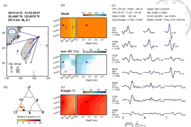
Figure 2.3 MT inversion results for the intermediate-depth earthquake on 2014/12/10 (ML=6.7) beneath the Ryukyu subduction zone.
The layout is the same as in Figure 2.2
Figure 2.3 shows the result of an intermediate depth earthquake occurring in offshore Northeast Taiwan on 2014/12/10. This earthquake was excluded in the previous BATS MT catalog because the original depth reported by CWB exceeds the BATS MT calculation range. Our new AutoBATS inversion can provide more
constraints to the subduction zone earthquakes. Unlike the shallow event shown in Figure 2, the misfit, non-DC component, and K-angle of this mid-focus offshore earthquake are relatively insensitive to velocity model, frequency bands, and focal depth, resulting in highly coherent focal mechanisms and less varied misfits (Figure 2.3). Because this earthquake is large in magnitude (Mw 6.0), filtering at a lower frequency band produces a smaller misfit as expected (Figure 2.3d). Although the
azimuthal coverage of stations is restricted in one quadrant, our MT solution and centroid depth estimation are both highly consistent with the solution from GCMT (Ekström et al., 2012). For intermediate depth earthquakes, the centroid depths are sometimes less well resolvable within our ±12 km scanning depth range because the misfit values are comparably small (Figure 2.3b). In addition to a reliable initial location from the CWB catalog, it is always recommended to consider other
independent constraints, such as the depth phases pP and sP observed at teleseismic distance, to further confirm the actual depth of the event.
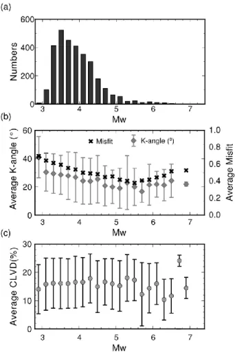
The AutoBATS MT inversion scheme shows superior capability for determining focal mechanisms. This study successfully resolved 3058 MTs (about 56%) out of 5500 CWB-reported earthquakes with acceptable data quality. Moreover, among these MT solutions, 87% have misfit smaller than 0.7 (above Category C in quality) and 99% have non-DC below 30% (above Class 4). Some resolved earthquakes are as small as MW 3.0 (Figure 2.4a). With the new AutoBATS catalog, we can further investigate whether the mean misfit, value of the CLVD component, and consistency of MT solutions (as described by the K-angle) have any relation with earthquake magnitudes. Figure 2.4b shows that the average misfit decreases from 0.7 to 0.4 as the moment magnitude increases from 3.5 to 5.6. This can be simply explained by the higher data quality against background noise for larger events. For earthquakes with MW ≥5.6, the average misfit increases again. This phenomenon may relate to the complexity of earthquake rupture, which often involves source directivity and multiple fault segments with different slip vectors, particularly in large events. Waveforms excited by complex source ruptures cannot be well simulated by a single focal mechanism, and so larger misfits may exist. In this case, the results of MT inversion
represent the overall effect of averaged rupture for the earthquakes. Like the features observed for misfit, the mean K-angle shows almost exactly the same trend; the values first decrease and then increase with magnitude (Figure 2.4b). The similarity between mean misfit and K-angle suggests that the stability and consistency of MT inversion results are mainly affected by the waveform quality for small-medium earthquakes and rupture complexity for larger earthquakes.
Contrarily, the mean CLVD appear to be a constant, independent of the magnitude of events (see Figure 2.4c). This phenomenon agrees with Kagan (2002), who
concluded that CLVDs are usually caused by artificial effects, except for
well-examined events. As already demonstrated in Figure 2.2b, the CLVD component of a shallow earthquake is easily affected by different inversion settings. For Taiwan earthquakes, we believe that the strong heterogeneity in tectonic structures and the long-period ambient noises for some stations are mostly responsible for the observed high CLVDs. The lower limit of the average K-angle or CLVD (defined by mean value minus a S.D.) for each Mw bin represents those earthquakes having overall consistent MTs or small CLVDs among all scanning settings. On the other hand, the upper bound (mean value plus a S.D.) reveals that the MT solutions are affected tremendously by different inversion settings. Again, the deviations (error bars) of the average K-angle and CLVD highlight the importance and necessity of probing the best solutions through comprehensive scanning on different inversion settings or parameters.
Figure 2.4 Number of events, Average K-angle and CLVD component with respect to Mw.
(a) Histogram showing the numbers of earthquakes with respect to MW (bin size = 0.2). (b) The relation of average misfit and K-angle with respect to MW based on all AutoBATS MT solutions. (c) The relation of average CLVD with respect to MW. Both error bars in (b) and (c) correspond to a standard deviation.