On: 24 December 2014, At: 18:33 Publisher: Taylor & Francis
Informa Ltd Registered in England and Wales Registered Number: 1072954 Registered office: Mortimer House, 37-41 Mortimer Street, London W1T 3JH, UK
Click for updates
Journal of Business Economics and
Management
Publication details, including instructions for authors and subscription information:
http://www.tandfonline.com/loi/tbem20
VaR and the cross-section of
expected stock returns: an emerging
market evidence
Dar-Hsin Chena, Chun-Da Chenb & Su-Chen Wuc a
Department of Business Administration, College of Business National Taipei University, 151 University Rd., San Shia, Taipei, 237 Taiwan. E-mail:
b
Department of Economics and Finance, College of Business, Tennessee State University, AWC Campus, 330 10th Avenue North, Nashville, TN, USA
c
Graduate Institute of Finance, National Chiao Tung University, Hsinchu, Taiwan
Published online: 08 Jul 2014.
To cite this article: Dar-Hsin Chen, Chun-Da Chen & Su-Chen Wu (2014) VaR and the cross-section of expected stock returns: an emerging market evidence, Journal of Business Economics and Management, 15:3, 441-459, DOI: 10.3846/16111699.2012.744343
To link to this article: http://dx.doi.org/10.3846/16111699.2012.744343
PLEASE SCROLL DOWN FOR ARTICLE
Taylor & Francis makes every effort to ensure the accuracy of all the information (the “Content”) contained in the publications on our platform. However, Taylor & Francis, our agents, and our licensors make no representations or warranties whatsoever as to the accuracy, completeness, or suitability for any purpose of the Content. Any opinions and views expressed in this publication are the opinions and views of the authors, and are not the views of or endorsed by Taylor & Francis. The accuracy of the Content should not be relied upon and should be independently verified with primary sources of information. Taylor and Francis shall not be liable for any losses, actions, claims, proceedings, demands, costs, expenses, damages, and other liabilities whatsoever or howsoever caused arising directly or indirectly in connection
substantial or systematic reproduction, redistribution, reselling, loan, sub-licensing, systematic supply, or distribution in any form to anyone is expressly forbidden. Terms & Conditions of access and use can be found at http://www.tandfonline.com/page/ terms-and-conditions
http://www.tandfonline.com/TBEM 2014 Volume 15(3): 441–459 doi:10.3846/16111699.2012.744343
VAR AND THE CROSS-SECTION OF EXPECTED STOCK
RETURNS: AN EMERGING MARKET EVIDENCE
Dar-Hsin Chen1, Chun-Da Chen2, Su-Chen Wu31Department of Business Administration, College of Business National Taipei University, 151 University Rd., San Shia, Taipei, 237 Taiwan
2Department of Economics and Finance, College of Business, Tennessee State University, AWC Campus, 330 10th Avenue North, Nashville, TN, USA
3Graduate Institute of Finance, National Chiao Tung University, Hsinchu, Taiwan E-mails: 1[email protected]; 2[email protected] (corresponding author)
Received 13 September 2011; accepted 16 October 2012
Abstract. In this paper we investigate the explanatory power of the market beta, firm
size, and the book-to-market ratio, as well as Value-at-Risk regarding the cross-sectional expected stock returns in a less developed stock market – Taiwan’s stock market. The main purpose is to examine whether the Value-at-Risk factor has marginal explanatory power related to the Fama-French three-factor model. The empirical results show that Value-at-Risk can account for the average stock returns at both 1% and 5% significance levels based on cross-sectional regression analysis. Moreover, from the perspective of the time series regression, the Value-at-Risk factor can also demonstrate the variation of the stock market, especially for the larger companies in the Taiwan stock market.
Keywords: CAPM, market beta, anomalies, emerging stock market, Value-at-Risk,
Fama-French factors.
Reference to this paper should be made as follows: Chen, D.-H.; Chen, C.-D.; Wu, S.-Ch.
2014. VaR and the cross-section of expected stock returns: an emerging market evidence,
Journal of Business Economics and Management 15(3): 441–459. JEL Classifications: G11, G12, G15.
Introduction
The prominent capital asset pricing model (CAPM) of Sharpe (1964), Lintner (1965), and Black (1972) has for decades been the major framework for analyzing the cross sectional variation in expected asset returns, but theory and practice might not always match. Fama and French (1992) draw two different conclusions regarding CAPM – that is, when one allows for variations in the CAPM market β that are unrelated to size, the univariate relationship between β and the average return for 1941–1990 is weak, and β does not suffice to explain this average return. They also find no cross-sectional return-beta relationship while controlling for size and the ratio of book-to-market equity (Chan, Chui 1996).
Several alternative risk factors have consequently been employed in the literature, for example, the size effect of Banz (1981) and Nunes et al. (2012). They finds the market value of equity (ME) and firm size provide an explanation of the cross-section of aver-age returns. Other variables such as the book-to-market equity ratio (BE/ME) (Fama, French 1992, 1993, 1995, and 1996; Rosenberg et al. 1985), the price/earnings ratio (Basu 1977), leverage (Bhandari 1988), Value-at-Risk (Bali, Cakici 2004), and profit-ability and investment patterns (Fama and French 2013) also have significant explana-tory power for making clear the average expected returns. Hung et al. (2004), on the other hand, control for the sign of realized market premia and use higher order asset pricing models to test CAPM.
More noteworthy is that the conception and utilization of Value-at-Risk (henceforth VaR) are designed to summarize the predicted maximum loss (or worst loss) over a target horizon within a given confidence interval (Jorion 2000). The movements of extreme price could bring serious results to some corporations and cause disastrous consequences for financial markets, although these cases are rare1. To a risk manager, a good measure of market risk is more than necessary. As such, VaR was first used by major financial firms and has become the most popular measurement for the risks of trading portfolios since the late 1980s.
Modeling portfolio risk with a traditional standard deviation (a good proxy of risk) measures implies in general that investors are concerned only with the average varia-tion in single stock returns. Financial data, however, exhibit fat-tailed and asymmetric distributions for market returns. For the last few decades, the popular and traditional measure of risk has been volatility, yet the main problem with volatility is that it does not involve the direction of an investment’s movement – a stock can be volatile, because it suddenly jumps higher. Investors are not distressed by gains! By assuming that inves-tors care about the likelihood of a really big loss, VaR answers the question, “What is my worst-case scenario?”
Traditional investment theory makes all possible uncertainty as risk in spite of the direction. As investors have shown, there is a problem if returns are not symmetrical. Investors worry about their losses “to the left” of the average, but they are not con-cerned with their gains “to the right” of the average. If investors are risk-averse, then they request greater compensation to hold stocks following higher downside risk. Many studies, including Campbell et al. (2001), find that market volatility increases in bear markets and recessions. Duffee (1995) also finds that idiosyncratic volatility increases in down markets. Both of these effects generate conditional beta that has little asymmetry across the downside and the upside. In particular, this paper measures VaR in terms of a company’s market value at risk. The VaR is related to the company’s stock price and it reflects the shareholders’ perception of risk. The downside focus separates the loss from the upside potential – namely, only the former truly constitutes risk and only negative surprises to the stock market represent potential litigation threats.
1 For instance, the New York stock market crashed in October 1987, and then, one decade later, the
Asian stock market crashed in 1997. The Enron scandal also caused the Dow Jones Industrial Av-erage (DJIA) to drop sharply. These crises have harmed thousands of companies and much of the value of their stocks has been wiped out within a short period of time.
Only a few studies have surprisingly so far looked at VaR (a proxy of risk, Bali, Cakici 2004). To the best of our knowledge, our attempt, which incorporates VaR as a measure of the risk explaining the portfolio expected returns in a less developed (emerging) stock market, is unique. In particular, the high volatility of stock returns occurs frequently in emerging stock markets. Under this circumstance, the dynamic risk management of VaR could access the real risks accurately. The daily price limit and short-sales constraint below last closing price are two major features in the Taiwan stock market. According to the information and overreaction hypothesis, the price limit does delay the process for prices to reflect intrinsic value. The short-sales constraint could prevent stock returns from any arbitrage momentum, but might tend to cause stock overvaluation and the overvaluation effect is more dramatic for individual stock reversely (Chang et al. 2007). On the strength of the reasons mentioned above, we believe that the VaR is relevant as a risk factor and an appropriate risk measurement, and it could also provide a good ex-planatory power in stock return and stock market variation (Jorion 1996). Another con-tribution of this paper is we fulfill the literature gap to examine whether the maximum potential loss measured by VaR plays a key role in explaining expected cross-sectional stock returns in Taiwan. Furthermore, this study also uses the Fama-French 3-factor model associated with VaR to investigate the cross-sectional variation at the firm level. The empirical results enrich our understanding of risk management and provide more evidence in emerging financial markets.
The remainder of this paper is organized as follows. Section 1 discusses the previous studies. Section 2 introduces the data, the variable definitions, and the models. The empirical results are presented in Section 3. Concluding remarks are given in the final section.
1. Literature review
Empirical research has provided several pieces of evidence that reject the validity of the Sharpe-Linter capital asset pricing model (CAPM). The existence of market fric-tions, the presence of irrational investors, and inefficient markets may distort the cross-sectional relationship between expected stock returns and market beta. This research discusses the relevant evidence reported in empirical studies.
1.2 Fama-French three factor model
CAPM employs a single factor, beta, to compare a portfolio with the market as a whole and was first introduced by Sharpe (1964) and Lintner (1965), but it oversimplifies the complex financial market. Fama and French (1992) start with the observation that two classes of stocks have tended to do better than the market as a whole: (1) small caps and (2) stocks with a high book-to-market equity ratio (BE/ME). They then add these two factors to CAPM to reflect a portfolio’s exposure – that is, the Fama-French three factor model, which corresponds to the following 3-factor regression:
[ ] ,
R RF a b RM RF− = + × − + ×c SMB d HML+ × (1)
where R is the portfolio’s return rate, RF is the risk-free return rate, and RM is the return of the aggregate stock market. The “three factor” beta is analogous to the classical beta, but not equal to it, since there are now two additional factors to do some of the work. The SMB (Small Minus Big) portfolio represents a zero- investment portfolio that is long in small-cap stocks and short in big-cap stocks. The HML (High Minus Low) port-folio represents a zero-investment portport-folio that is long in high book-to-market stocks (so-called “Value” stocks) and short in low book-to-market stocks (so-called “Growth” stocks). The Fama-French model is based on the observation that small cap stocks and “Value” stocks historically tend to do better than the market as a whole. While R2 for CAPM usually takes values of around 0.85, the Fama-French model is capable of ac-counting for almost all variation in individual assets2.
1.2 Application of Value-at-Risk (VaR)
The VaR analysis originated with the variance-covariance model introduced by J.P. Mor-gan’s RiskMetrics in 1993. The variance-covariance approach to calculating risk could be traced back to the modern portfolio theory by Markowitz (1959), in which most of today’s risk managers are conversant. Engle and Manganelli (2004) further extend the quantile regression to model the VaR directly instead of modeling the underlying volatility generating process and also introduce the conditional autoregressive Value-at-Risk (CAViaR) model. Sequentially, Bali and Weinbaum (2005), Bali and Cakici (2004 and 2006), Lim and Tan (2007), and Bail et al. (2009) also employ the concept of conditional VaR to measure idiosyncratic risk and market returns. It is worth noting that Bali and Cakici (2004) argue that the VaR captures the cross-sectional differences in expected stock returns of firms on the U.S. three major stock exchanges, whereas the market beta and total volatility have no power in explaining the firm’s average stock returns. Therefore, this study is strongly motivated by their vigorous findings and fol-lows a similar methodology to apply Taiwan data that compares the prediction ability (in terms of the R2 value) of beta, size, BE/ME, and VaR and explains the cross-sectional variation in portfolio returns3.
2. Data, variable definitions and methodology 2.1. Data
According to Bali and Cakici (2004), this paper examines whether the market factor (beta), firm size, BE/ME, and VaR provide different explanatory powers to the average stock returns under diverse company characteristics in an emerging market – Taiwan. The stock returns covered in this study include the all listed stocks of TSEC (Taiwan Stock Exchange). Regarding the sample period, to avoid possible abnormal trading 2 For other important relevant studies following the Fama-French three factor model, please refer to
Heston et al. (1999) in beta, Berk (1995), Chen and Zhang (1998), Chiu and Wei (1998), Rouwen-horst (1999), Jarrett and Schilling (2008), and Bistrova et al. (2011) in size effect, and Lakonishok
et al. (1994), Fama and French (1993 and 1995), and Roll (1995) in the BE/ME ratio effect. 3 Please refer to the page 58 of Bali and Cakici (2004) for the detailed VaR definitions and calculations.
activities during the 1997 Asia financial crisis period (1997 to 1998, when the total market value lost over 40%), the sample period for this study covers seventeen years, from 1991 to 2009. The estimation period spans from January 1991 through December 1995, while the test period extends from January 1996 to December 20094. The Taiwan
Economic Journal (TEJ) database provides these firms’ stock returns.
2.2. Variable definitions Systematic risk (Beta)
Following Fama and French (1992), this study sorts all the stocks by size (the market value of equity) to determine the stocks’ quintile breakpoints, because the size differ-ences may be attributed to a wide range of average returns and βs (Chan and Chen, 1991). We then subdivide each size quintile into five portfolios on the basis of pre-ranking betas for all the stocks. The pre-pre-ranking betas are calculated by monthly returns of five years ending in December 1995 and 144 post-ranking monthly returns for each of 25 portfolios are estimated from January 1996 to December 20095. We follow Allen and Cleary (1998) to evaluate beta incorporating Scholes and Williams (1997) as the sum of the slopes in the regression of portfolio returns on portfolios6.
Size
Following the previous studies, we evaluate size, the market value of a firm’s outstand-ing shares, with the natural logarithm of the market value of equity.
Book-to-market equity (BE/ME)
Book-to-market equity (BE/ME) is the natural logarithm of the ratio of the book value of equity plus deferred taxes over the market value of equity, which involves account-ing- and market-based variables. This paper uses a firm’s market equity at the end of December of the previous year to compute its BE/ME.
Value-at-Risk (VaR)
In this paper we follow the method of Bali and Cakici (2004) to estimate VaR7. After obtaining the VaR for each stock, we rank and place VaR into 5 quintile portfolios. Port-4 To be included in the sample, for a given month a stock has to satisfy several criteria. First, the
stock returns over the previous 60 months are available. Second, data are available from TEJ to calculate the BE/ME ratio as of December of the previous year. Finally, we include only securities defined by TEJ as ordinary common shares.This screening process yields averages of 202 stocks per month.
5 The choice of using portfolios instead of individual shares is dictated by the evidence of Griffin
and Lemmon (2002) which shows that this is the way the sampling error is reduced. Additionally, using portfolios also facilitates a comparison with past studies in the field, as the majority of these studies use portfolios instead of individual stocks. Further advantages of using portfolios instead of individual firms in the regressions include the following: 1. A pooled sample of individual firms used in CSR analysis allows us to eliminate the potential threat posed by temporal and firm-specific effects in terms of biasing the results. 2. There is significantly less computational effort in using portfolios instead of individual stocks in the regression analysis.
6 Due to limited space, please refer to Allen and Cleary (1998) for the detailed beta estimation. 7 We further use EWMA (exponentially weighted moving average) to check the performance of our
model and the results are similar.
folio 1 has the lowest VaR and portfolio 5 has the highest VaR. The portfolio formation procedure is very similar to Fama and French (1992), except that they update their port-folios annually, whereas we update ours on a monthly basis. The estimation period and test period of VaR respectively span from 1991 to 1995 and from 1996 through 2009. We calculate the one-month-ahead portfolio returns from 1996 to 2009 with 144 time series for the 5 equally-weighted portfolios based on VaRs and find that the portfolios with the higher VaR have greater rates of return.
2.3. Methodology
Cross-sectional regression
This paper utilizes Fama-MacBeth (1973) (hereafter FM) regressions to examine wheth-er the beta, size, BE/ME, 1% VaR, 5% VaR, and 10% VaR can provide large and statistically significant cross-sectional variations in expected stock returns. Monthly cross-sectional regressions are run for the following econometric specifications:
, 1 , , 1
j t t t j t j t
R + = ω + γ X + ε + , (2)
1% 5% 10%
BETA,ln(ME),ln(BE/ME),VaR ,VaR ,and VaR
X = ,
where Rj t, 1+ is the realized average return on stock j in month t + 1, and BETA and ln(ME) are the respective full-sample pre-ranking beta and the natural logarithm of mar-ket equity. VaR(α) is – 1 times the maximum likely loss (VaR) with the loss probability level α =1%, 5%, and 10%, and εj t+, 1 is the residual series from the cross-sectional regressions.
Size-BE/ME portfolios and VaR-BE/ME portfolios
In the study we follow Fama and French (1993) to construct the factor mimicking port-folio. Fama and French (1993, 1995, 1996) also indicate the importance and calculations of RMRF, SMB, and HML. To test the performance of VaR based on the 25 portfolios of Fama and French (1993), this study devises a factor, HVARL (high VaR minus low VaR), that is designed to mimic the risk factor in returns related to Value-at-Risk and is defined as the difference between the simple average returns on the high-VaR and low-VaR portfolios. The construction of a 5% low-VaR portfolio is similar to the construction of Fama and French’s size portfolios. In December of each year t from 1996 to 2009, this study ranks all stocks according to a 5% VaR. The median 5% VaR figure is used to divide the stocks into two groups – the high VaR and low VaR groups.
Three-factor model and four-factor model
This study performs a four-step analysis of the various factors (RMRF, HVARL, SMB, and HML) in explaining stock returns and then examines the three-factor and four-factor models. The three-four-factor model suggested by Fama and French (1993) provides an alternative to the CAPM for the estimation of expected returns. This model includes two additional factors to explain excess return: size and the book-to-market ratio. The Fama and French model is of primary interest to us as one of the objectives of the pa-per is to assess its implications for an investor’s investment decision. The explanatory variables in the time series regressions include not only the returns on a market portfolio of stocks, but also the mimicking portfolio returns for size and book-to-market. The
four-factor model adds another risk factor, i.e. HVARL, into the three-factor model. The risk factor is a mimicking portfolio that follows Bali and Cakici (2004) as follows:
( ) ( ) [ ( ) ( )] ( ).
R t −RF t = + ×a b RM t −RF t + ×c SMB d HML e HVARL u t+ × + × + (3) 3. Empirical results
3.1. VaR and cross-sectional regression
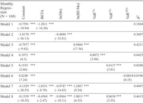
This section shows the results of the Fama and MacBeth regressions (estimated by Or-dinary Least Squares method) of excess returns on characteristics that are best known to be associated with expected returns – namely, the beta, firm size, BE/ME, and VaR (1%, 5%, and/or 10%) variables. Table 1 presents the time series average value of γt, the t-statistics, and the time series averages of the determination coefficient (R2) over
Table 1. Cross-sectional regressions of stock returns on Beta, size, BE/ME, and VaR Monthly
Regres-sion
(N = 168) Constant BETA ln(Me) ln(BE/Me) 1%RVa 5%VaR 10%VaR 2R
Model 1 –0.7591 (–10.94)*** –1.2811(–16.20)*** 0.1684 Model 2 –3.8170 (–26.13)*** (–33.81)–0.4888*** 0.3607 Model 3 –0.7977 (–9.82) *** (17.36)0.9404*** 0.4211 Model 4 0.1972 (4.3) *** 0.0072(3.08) *** 0.0425 Model 5 0.1555 (2.66) *** 0.0137(3.01)*** 0.0280 Model 6 0.4240 (7.24) *** –0.0034(0.35) 0.0196 Model 7 –4.1359 (–28.55)*** –1.0331(–8.70) *** –0.9747(–14.45)*** 1.2487(9.34) *** 0.4497 Model 8 –0.1359 (–10.35)*** –0.4569(–2.47) ** –0.8964(–10.11)*** 1.0013(6.55) *** 0.0654(3.35)*** 0.4613
Notes: ***, **, and * mean significantly different from zero at the 0.01, 0.05, and 0.10 levels,
respec-tively. This table reports the time-series average of the month-by-month regression slopes from January 1996 to December 2009. The dependent variables are the monthly average returns on individual stocks. The independent variables include beta, firm size, the book-to-market ratio (BE/ME), and VaRα, where
1%, 5%, and 10%.
α = The betas that correspond to the portfolio they belong to are assigned to in-dividual stocks. The size is the natural log of the market value. The BE/ME is the natural log of the book-to-market value. The VaR is calculated using the historical simulation method (the tails of the empirical return distribution). We use OLS (ordinary least squares) method to estimate regressions of the following form: Rj t, = ω + γ ×t t Xj t, + εj t,, where X contains 6 independent variables. The
t-statistic reported in the parentheses is the average slope divided by its time-series standard error. For robustness, we also try 1% VaR and 10% VaR in Model 8, but the results have no significant change.
the 144 months in the sample. The t-statistics shown in the parentheses are the time series average values of γt divided by the corresponding time-series standard errors. As can be seen from the estimated slopes of beta, ln(ME) and ln(BE/ME) are all highly significant at the 1% level. The average slopes provide standard Fama-MacBeth tests for determining which explanatory variables had, on average, non-zero expected return premiums during the January 1996 to December 2009 period. As expected, there is a negative relationship between the realized stock returns and beta. The empirical evi-dence shows that the lower the sensitivity is of the asset return, the greater the realized return will be (Fama, MacBeth 1973; Banz 1981). Meanwhile, the average slope for the monthly regressions of the realized returns and size, ln(ME), is negative and about –0.49, with a t-statistic of –33.81. We believe that size is related to profitability. On average, the profitability of larger-cap stocks in the Taiwan stock market is less than that of smaller-cap stocks. This result also shows that, for a firm with larger capitaliza-tion, the performance seems lower than for the small firm from the viewpoint of the cross-sectional regressions.
The average slope based on the univariate regressions of the monthly return on ln(BE/ ME) is about 0.94, with a t-statistic of 17.36, implying that the risk captured by BE/ ME is the relatively distressed factor of Chan and Chen (1991). They postulate that the earning prospects of firms are associated with a risk factor in the returns. Firms that the market judges to have poor prospects, signaled here by low stock prices and high BE/ME ratios, have higher expected returns (they are penalized with higher costs of capital) than firms with strong prospects. It is also possible that BE/ME only captures the unraveling of irrational market whims regarding the prospects of firms. This result accords with the view put forward by Fama and French (1992) that BE/ME has a stronger role in explaining average stock returns than size. Furthermore, as we move to a lower significance level (higher confidence level), the VaR estimation becomes more important in explaining the cross-sectional average stock returns. We can see that the VaR(α) is significant when α is 1% and 5%. The results of the positive coefficients of VaR indicate that the greater a stock’s potential fall in value is, the higher the expected return should be. In addition, we further report multivariate cross-sectional regression results as Model 7 and Model 8. The result shows that the VaR does provide a higher explanatory power to the stock monthly average returns. The R2 of Model 7 and Model 8 are higher than those of Model 1 to Model 6.
3.2. VaR and time-series variation of expected returns
In time-series regressions, the slopes and R2 values are direct evidence as to whether different risk factors capture a common variation in stock returns. This study examines the explanatory power of stock market factors. Table 2 of Panel A shows the simple statistics of RMRF, SMB, HML and HVARL. The average value of the market risk pre-mium is 1.28% per month. This study also calculates the correlations between RMRF, SMB, HML, and HVARL. Table 2 of Panel B presents the correlation coefficients for the factors used. The last row shows that HVARL is positively correlated with RMRF and SMB, whereas it is negatively correlated with HML. A notable point is that the positive relationship between HVARL and SMB is much stronger than the negative relationship between HVARL and HML.
Table 2. Time series regressions – descriptive statistics Panel A: Descriptive Statistics
Variable N Mean Std. Dev. minimum Maximum
RMRF 132 1.2753 9.0405 –23.3456 24.7122
SMB 132 –0.6008 4.6622 –18.1625 10.5123
HML 132 3.0023 6.2125 –19.4860 21.4324
HVARL 132 0.4437 5.6937 –17.0467 20.1614
Panel B: Pearson Correlation Coefficients, N = 144 Prob > |r| under H0 : ρ = 0 RMRF SMB HML HVARL RMRF ---SMB –0.0633 ---HML –0.0747 –0.5971 * ---HVARL 0.6754 ** 0.4769 ** –0.3760 *
---Notes: This table gives the correlation coefficients calculated from the sample. An asterisk indicates
that the correlation coefficient is significant (i.e. the p-value is less than 0.05). ***, **, and * means significantly different from zero at the 0.01, 0.05, and 0.10 levels, respectively. This table presents simple summary statistics for the stocks in the sample. The six size-PB portfolios (S/L, S/M, S/H, B/L, B/M, and B/H) are formed in December of each year t-1 and value-weighted monthly returns are calculated from January to December of year t. Panel A presents the basic statistics of the four factors. Panel B presents the Pearson correlation coefficients that are calculated based on monthly returns for each of the factors RMRF, SMB, HML, and HVARL. The sample period extends from January 1996 to December 2009 exclusive of 1997 and 1998 – there being 144 monthly observations.
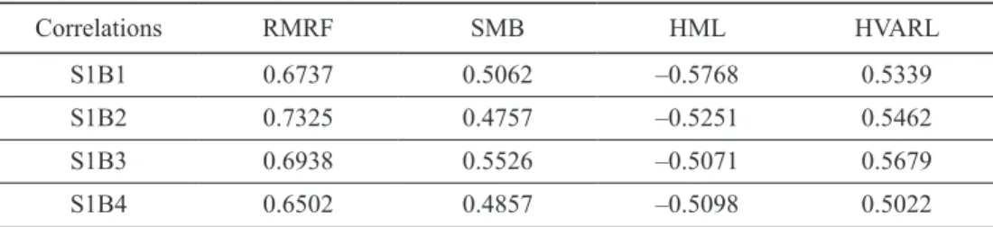
To compare the relative performances of HVARL, RMRF, SMB, and HML, this study calculates the correlations between the returns for the 25 portfolios of Fama and French (1993) and the various factors. Table 3 shows that, not surprisingly, the excess return on the market portfolio of stocks, RMRF, captures more common variations in stock returns, on average, than HVARL, HML, and SMB. The average correlation between the returns for the 25 portfolios and RMRF is 0.7673, whereas the average correlation between HVARL and the monthly returns on the 25 portfolios is 0.4824. Furthermore, the average correlation is 0.3011 for SMB and –0.3809 for HML. Clearly, HVARL as a single factor is superior to SMB and HML in explaining the time-series variation in stock returns.
Table 3. Correlations of 25 portfolio returns with RMRF, SMB, HML, and HVARL
Correlations RMRF SMB HML HVARL
S1B1 0.6737 0.5062 –0.5768 0.5339
S1B2 0.7325 0.4757 –0.5251 0.5462
S1B3 0.6938 0.5526 –0.5071 0.5679
S1B4 0.6502 0.4857 –0.5098 0.5022
Correlations RMRF SMB HML HVARL S1B5 0.6966 0.4260 –0.3111 0.4999 S2B1 0.7463 0.4361 –0.5201 0.4929 S2B2 0.7591 0.4641 –0.4774 0.5686 S2B3 0.6941 0.4139 –0.4975 0.4497 S2B4 0.7451 0.3519 –0.1891 0.4630 S2B5 0.7502 0.4537 –0.6120 0.5643 S3B1 0.7338 0.3796 –0.4170 0.4759 S3B2 0.7667 0.3593 –0.3467 0.4469 S3B3 0.7718 0.2150 –0.1478 0.4606 S3B4 0.7651 0.3717 –0.6163 0.5862 S3B5 0.7728 0.3232 –0.5354 0.5427 S4B1 0.8096 0.2052 –0.3373 0.4011 S4B2 0.8132 0.0840 –0.0675 0.5476 S4B3 0.8299 0.1710 –0.4630 0.4536 S4B4 0.8543 0.0677 –0.2828 0.3222 S4B5 0.8305 0.0129 –0.2229 0.2653 S5B1 0.8879 –0.3264 0.2379 0.4791 S5B2 0.6737 0.5062 –0.5768 0.5339 S5B3 0.7325 0.4757 –0.5251 0.5462 S5B4 0.6938 0.5526 –0.5071 0.5679 S5B5 0.6502 0.4857 –0.5098 0.5022 Average 0.7673 0.3011 –0.3809 0.4824
Notes: S1B1 (S5B5) denotes a size-BE/ME portfolio that belongs to the smallest (largest) size quintile
and lowest (highest) BE/ME quintile.
3.3. Properties of portfolios formed based on size and pre-ranking β
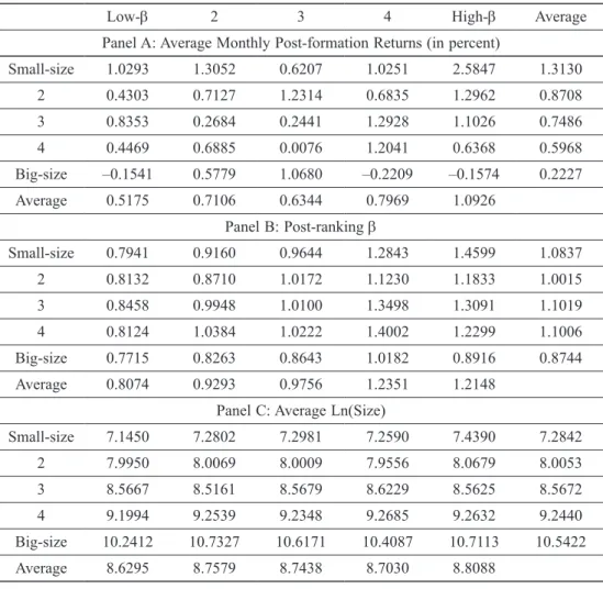
Fama and French (1992) find that after controlling for the size and book-to-market ef-fects, beta seems to have no power to explain the average returns on a security. This finding is an important challenge to the notion of a rational market, since it seems to imply that a factor that should affect return – systematic risk – does not seem to matter. Table 4 shows that forming portfolios on size and pre-ranking βs, rather than on size alone, magnifies the range of full-period post-ranking βs. The all column and row shows statistics for equal-weighted size-decile portfolios and for equal-weighted portfolios of the stocks in each β group respectively.
The average row of Panel B of Table 4 shows that the portfolio beta of each beta group averaged across the 5 different-sized portfolios steadily increases from 0.81 to 1.21. End of Table 3
The average row in Panel C shows that the average portfolio size within each beta group is almost identical, ranging from 8.63 to 8.81. This allows us to interpret Panel A as a test of the net effect of beta on average returns holding size fixed. Panel A of Table 4 clearly shows that, for the period 1996–2009, average returns are not positively related to beta. The highest-beta portfolios do not have the highest returns, and this occurs
Table 4. Properties of portfolios formed on size and pre-ranking β: stocks sorted by size (down) then pre-ranking β (across), 1996–2009
Low-β 2 3 4 High-β Average
Panel A: Average Monthly Post-formation Returns (in percent)
Small-size 1.0293 1.3052 0.6207 1.0251 2.5847 1.3130 2 0.4303 0.7127 1.2314 0.6835 1.2962 0.8708 3 0.8353 0.2684 0.2441 1.2928 1.1026 0.7486 4 0.4469 0.6885 0.0076 1.2041 0.6368 0.5968 Big-size –0.1541 0.5779 1.0680 –0.2209 –0.1574 0.2227 Average 0.5175 0.7106 0.6344 0.7969 1.0926 Panel B: Post-ranking β Small-size 0.7941 0.9160 0.9644 1.2843 1.4599 1.0837 2 0.8132 0.8710 1.0172 1.1230 1.1833 1.0015 3 0.8458 0.9948 1.0100 1.3498 1.3091 1.1019 4 0.8124 1.0384 1.0222 1.4002 1.2299 1.1006 Big-size 0.7715 0.8263 0.8643 1.0182 0.8916 0.8744 Average 0.8074 0.9293 0.9756 1.2351 1.2148
Panel C: Average Ln(Size)
Small-size 7.1450 7.2802 7.2981 7.2590 7.4390 7.2842 2 7.9950 8.0069 8.0009 7.9556 8.0679 8.0053 3 8.5667 8.5161 8.5679 8.6229 8.5625 8.5672 4 9.1994 9.2539 9.2348 9.2685 9.2632 9.2440 Big-size 10.2412 10.7327 10.6171 10.4087 10.7113 10.5422 Average 8.6295 8.7579 8.7438 8.7030 8.8088
Notes: At the end of year t–1, the stocks obtained from the TEJ are assigned to 5 size portfolios. Each
size quintile is subdivided into 5 β portfolios using the pre-ranking β of individual stocks estimated with 60 monthly returns ending in December of year t-1. The equal-weighted monthly returns on the resulting 25 portfolios are then calculated for year t. The average returns are the time-series average of the monthly returns, in percentage form. The post-ranking βs use the full 1996–2009 sample of post-ranking returns for each portfolio. The pre- and post-ranking βs are the sum of the slopes from a regression of monthly returns for the current and prior months’ value-weighted market return. The average size of a portfolio is the time-series average of each month’s average value of ln(Size) for a stock within the portfolio. Size is dominated in millions of TWD. There are, on average, about 5 stocks in each size-β portfolio in each month.
in the fourth-beta portfolios. The results do not support the central prediction of the CAPM, because average stock returns are not positively related to the market beta at the portfolio level. The CAPM insight is that volatility arising from specific events (called specific or idiosyncratic risk) can be eliminated in a diversified portfolio, and that inves-tors will not be paid for bearing these risks with extra returns. This result will support us as we continue to further discuss the three- and four-factor models. We should note that average monthly post-formation returns seem to be negatively correlated with firm size. The smallest size quintile, on average, has the highest average return (1.31% per month) and the biggest size quintile has the lowest average return (0.22% per month). 3.4. Properties of portfolios formed on VaR and pre-ranking β
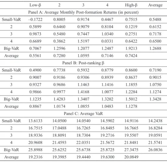
Table 5 of Panel A reports that when common stock portfolios are formed on 5% VaR, the average stock returns are positively related to VaR. Going from the lowest 5% VaR quintile to the highest 5% VaR quintile, the average stock returns from VaR portfolios increase from 0.55% per month to 1.27% per month monotonically. This result sup-ports our argument to the effect that if investors are more averse to the risk of losses on the downside than of gains on the upside, i.e. a higher VaR, then investors should demand greater compensation. Furthermore, we see that the greatest average monthly post-formation return is about 1.92%, and not surprisingly it is apparent in the high-est VaR-BE/ME group. However, the average monthly post-formation returns are not similar within the same β quintile. For the smallest 5% VaR quintile, the highest β does not have the largest stock returns. Beta seems to have much less power to explain the average stock returns after controlling for the 5% VaR and book-to-market effects. These results inform us that the more a stock can potentially fall in value, the higher the expected return should be.
3.5. Main model results: three and four-factor models
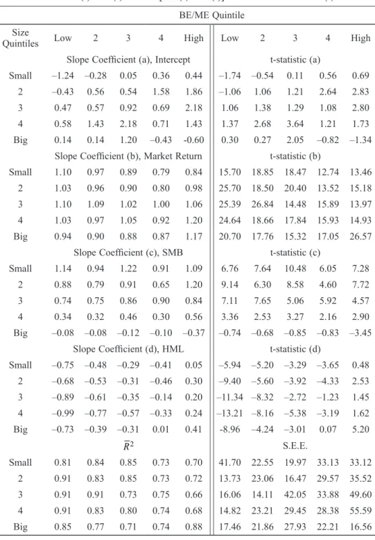
Table 6 presents estimates from the three-factor model in which the excess returns on 25 portfolios are regressed on RMRF, SMB, and HML. Table 6 demonstrates that most of the coefficients for the three Fama-French factors (coefficient (b) is for RMRF, coef-ficient (c) is for SMB, and coefcoef-ficient (d) is for HML) are highly significant. The lower BE/ME quintile and bigger size quintile portfolios capture between 70% and 90% of the variations in terms of the R2 values. However, the higher BE/ME quintile and smaller size quintile seem to leave 30–40% of variations that cannot be explained by Fama and French’s three-factor model. Furthermore, the results indicate that, when controlling for the BE/ME effect, the SMB factor is highly significant. What is initially surprising, however, is the fact that SMB seems to work in a reverse manner than what would be expected, i.e. small firms have on average higher returns than big firms do. This can be seen by looking at the coefficients for SMB, which go from positive to negative when moving from small stock portfolios to big stock portfolios and after taking into account the fact that the size premium is negative during our sample period. On the other hand, when controlling for size, the HML factor clearly captures the higher returns for the high BE/ME portfolios as compared to the low BE/ME stocks. Subsequently, we will continue to see if another factor – the VaR – can enhance and capture the variations.
Therefore, SMB, the mimicking return for the size factor, has more power than HML. Not surprisingly, the slopes on HML are systematically related to BE/ME. In every size quintile of stocks, the HML slopes increase monotonically from lower to higher BE/ ME quintiles.
Table 5. Properties of portfolios formed on VaR and pre-ranking β: stocks sorted by VaR (down) then pre-ranking β (across), 1996–2009
Low-β 2 3 4 High-β Average
Panel A: Average Monthly Post-formation Returns (in percent)
Small-VaR –0.1722 0.8005 0.9174 0.4467 0.7515 0.5488 2 0.5899 0.6460 0.9079 0.8104 0.1219 0.6152 3 0.9873 0.5480 0.7447 1.0340 0.2751 0.7178 4 0.6689 0.3862 1.5197 0.0331 0.6422 0.6500 Big-VaR 0.7067 1.2596 1.2077 1.2487 1.9213 1.2688 Average 0.5561 0.7280 1.0595 0.7146 0.7424 Panel B: Post-ranking β Small-VaR 0.4900 0.7738 0.5932 0.8779 0.8600 0.7190 2 0.9007 0.9186 0.9306 0.8939 0.8637 0.9015 3 0.9327 0.9686 1.1463 1.1416 1.1855 1.0750 4 0.9866 0.9977 1.4168 1.0077 1.2284 1.1274 Big-VaR 1.1235 1.4283 1.3407 1.3202 1.5012 1.3428 Average 0.8867 1.0174 1.0855 1.0483 1.1278
Panel C: Average VaR
Small-VaR 13.6133 14.0500 14.0540 14.5902 14.9116 14.2438 2 16.7515 17.0488 16.7265 16.8485 16.7665 16.8284 3 18.9336 18.8091 18.7304 19.2716 19.5507 19.0591 4 20.9608 21.4593 22.0351 21.5672 21.8481 21.5741 Big-VaR 25.8988 25.6252 25.6738 25.8725 27.3475 26.0836 Average 19.2316 19.3985 19.4440 19.6300 20.0849
Notes: The formation of the VaR-beta portfolios is similar to that of the size-β portfolios. At the
end of year t-1, stocks are sorted by their 5% VaR and assigned to 5 portfolios. Each VaR quintile is subdivided into 5 β portfolios using the pre-ranking β ending in December of year t-1. The equal-weighted monthly returns on the resulting 25 portfolios are then calculated for year t. The average returns are the time-series average of the monthly returns, in percentage form. The post-ranking βs use the full 1996-2009 sample of post-ranking returns for each portfolio. The pre- and post-ranking βs are the sum of the slopes from a regression of monthly returns on the current and prior months’ value-weighted market return. The average 5% VaR of a portfolio is the time-series average of each month’s average value of 5% VaR for stock in the portfolio. There are, on average, about 5 stocks in each VaR-β portfolio each month.
Table 6. Three-factor model: regression of excess stock returns on the excess stock-market return, SMB, and HML (Jan. 1996 to Dec. 2009, N = 144)
Panel A: R t( )−RF t( )= + ×a b RM t[ ( )−RF t( )]+ ×c SMB d HML u t+ × + ( ) BE/ME Quintile
Size
Quintiles Low 2 3 4 High Low 2 3 4 High
Slope Coefficient (a), Intercept t-statistic (a)
Small –1.24 –0.28 0.05 0.36 0.44 –1.74 –0.54 0.11 0.56 0.69
2 –0.43 0.56 0.54 1.58 1.86 –1.06 1.06 1.21 2.64 2.83
3 0.47 0.57 0.92 0.69 2.18 1.06 1.38 1.29 1.08 2.80
4 0.58 1.43 2.18 0.71 1.43 1.37 2.68 3.64 1.21 1.73
Big 0.14 0.14 1.20 –0.43 -0.60 0.30 0.27 2.05 –0.82 –1.34
Slope Coefficient (b), Market Return t-statistic (b)
Small 1.10 0.97 0.89 0.79 0.84 15.70 18.85 18.47 12.74 13.46
2 1.03 0.96 0.90 0.80 0.98 25.70 18.50 20.40 13.52 15.18
3 1.10 1.09 1.02 1.00 1.06 25.39 26.84 14.48 15.89 13.97
4 1.03 0.97 1.05 0.92 1.20 24.64 18.66 17.84 15.93 14.93
Big 0.94 0.90 0.88 0.87 1.17 20.70 17.76 15.32 17.05 26.57
Slope Coefficient (c), SMB t-statistic (c)
Small 1.14 0.94 1.22 0.91 1.09 6.76 7.64 10.48 6.05 7.28
2 0.88 0.79 0.91 0.65 1.20 9.14 6.30 8.58 4.60 7.72
3 0.74 0.75 0.86 0.90 0.84 7.11 7.65 5.06 5.92 4.57
4 0.34 0.32 0.46 0.30 0.56 3.36 2.53 3.27 2.16 2.90
Big –0.08 –0.08 –0.12 –0.10 –0.37 –0.74 –0.68 –0.85 –0.83 –3.45
Slope Coefficient (d), HML t-statistic (d)
Small –0.75 –0.48 –0.29 –0.41 0.05 –5.94 –5.20 –3.29 –3.65 0.48 2 –0.68 –0.53 –0.31 –0.46 0.30 –9.40 –5.60 –3.92 –4.33 2.53 3 –0.89 –0.61 –0.35 –0.14 0.20 –11.34 –8.32 –2.72 –1.23 1.45 4 –0.99 –0.77 –0.57 –0.33 0.24 –13.21 –8.16 –5.38 –3.19 1.62 Big –0.73 –0.39 –0.31 0.01 0.41 -8.96 –4.24 –3.01 0.07 5.20 2 R S.E.E. Small 0.81 0.84 0.85 0.73 0.70 41.70 22.55 19.97 33.13 33.12 2 0.91 0.83 0.85 0.73 0.72 13.73 23.06 16.47 29.57 35.52 3 0.91 0.91 0.73 0.75 0.66 16.06 14.11 42.05 33.88 49.60 4 0.91 0.83 0.80 0.74 0.68 14.82 23.21 29.45 28.38 55.59 Big 0.85 0.77 0.71 0.74 0.88 17.46 21.86 27.93 22.21 16.56
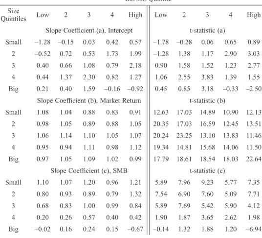
Table 7 presents the parameter estimates, t-statistics, R2 values, and standard errors of estimate (S.E.E.) from the time series regressions of excess stock returns on RMRF, SMB, HML, and HVARL. As shown in Table 7, the slope coefficients for the market factor, RMRF, are highly significant. Most of the slope coefficients for SMB and HML factor are also significant. A notable point is that, for the lowest size-quintile, none of the HVARL slopes are significant, but the rest of 20 HVARL slopes are significant. The
2
R values of the four-factor model are greater than those of the three-factor model. When viewed at the portfolio level, these empirical results show that the VaR factor plays an important role in firms especially with larger capitalization. This could be the reason why either the concept of VaR is not very familiar to individual investors since they are the major participants in the Taiwan stock market or else larger companies always pay much attention to VaR in order to control for downside risk. However, after the New Basle II Accord was implemented at the end of 2006, VaR is looking to play an increasingly important role to stock returns in the future.
Table 7. Four-factor model: regression of excess stock returns on the excess stock-market return, SMB, HML, and HVARL (Jan. 1996 to Dec. 2009, N = 144)
Panel A: R t( )−RF t( )= + ×a b RM t[ ( )−RF t( )]+ ×c SMB d HML e HVARL u t+ × + × + ( ) BE/ME Quintile
Size
Quintiles Low 2 3 4 High Low 2 3 4 High
Slope Coefficient (a), Intercept t-statistic (a)
Small –1.28 –0.15 0.03 0.42 0.57 –1.78 –0.28 0.06 0.65 0.89
2 –0.52 0.72 0.53 1.73 1.99 –1.28 1.38 1.17 2.90 3.03
3 0.40 0.66 1.08 0.79 2.18 0.90 1.58 1.52 1.23 2.77
4 0.44 1.37 2.30 0.82 1.27 1.06 2.55 3.83 1.39 1.55
Big 0.21 0.40 1.59 –0.16 –0.92 0.45 0.85 3.18 –0.33 –2.50
Slope Coefficient (b), Market Return t-statistic (b)
Small 1.08 1.04 0.88 0.83 0.91 12.63 17.03 14.89 10.90 12.13
2 0.98 1.05 0.89 0.88 1.05 20.35 17.03 16.59 12.45 13.51
3 1.06 1.14 1.10 1.05 1.07 20.24 23.25 13.10 13.83 11.46
4 0.95 0.94 1.11 0.98 1.12 19.34 14.81 15.68 14.06 11.50
Big 0.97 1.05 1.09 1.02 0.99 17.79 18.61 18.54 18.03 22.64
Slope Coefficient (c), SMB t-statistic (c)
Small 1.10 1.07 1.20 0.96 1.21 5.89 7.96 9.23 5.77 7.35
2 0.80 0.93 0.89 0.79 1.32 7.54 6.90 7.60 5.09 7.71
3 0.68 0.83 1.00 0.99 0.84 5.89 7.69 5.42 5.90 4.12
4 0.20 0.26 0.57 0.40 0.42 1.90 1.87 3.65 2.62 1.98
Big –0.02 0.16 0.24 0.15 –0.67 –0.14 1.32 1.88 1.20 –6.94
Size
Quintiles Low 2 3 4 High Low 2 3 4 High
Slope Coefficient (d), HML t-statistic (d)
Small –0.74 –0.52 –0.28 –0.42 0.02 –5.77 –5.58 –3.16 –3.72 0.21
2 –0.66 –0.56 –0.31 –0.50 0.26 –9.09 –6.06 –3.81 –4.66 2.26
3 –0.87 –0.63 –0.38 –0.16 0.20 –11.02 –8.56 –3.01 –1.42 1.42
4 –0.96 –0.75 –0.60 –0.36 0.27 –13.03 –7.90 –5.60 –3.41 1.85
Big –0.75 –0.45 –0.40 –0.06 0.49 –9.06 –5.31 –4.54 –0.67 7.44
Slope Coefficient (e), HVARL t-statistic (e)
Small 0.07 –0.25 0.05 –0.11 –0.24 0.43 –2.19 0.43 –0.76 –1.68 2 0.27 –0.29 0.02 –0.27 –0.34 1.84 –2.50 0.22 –2.03 –1.99 3 0.22 –0.16 –0.29 –0.18 –0.33 1.75 –1.69 –1.84 –1.27 –2.03 4 0.36 –0.14 –0.21 –0.35 0.38 2.84 –1.95 –1.67 –1.73 1.66 Big –0.23 –0.49 –0.72 –0.50 0.60 –2.24 –4.62 –6.45 –4.67 7.26 2 R S.E.E. Small 0.81 0.85 0.85 0.73 0.70 42.03 21.76 20.12 33.27 32.55 2 0.92 0.84 0.85 0.74 0.73 13.42 21.96 16.62 28.71 34.98 3 0.91 0.91 0.74 0.75 0.66 15.97 13.87 41.10 33.69 50.08 4 0.91 0.83 0.81 0.74 0.68 13.87 23.23 29.04 28.02 54.88 Big 0.85 0.81 0.79 0.78 0.92 17.37 18.28 20.08 18.50 11.06 Conclusions
By focusing on downside risk as an alternative measure of risk measured by VaR, this paper investigates whether the new VaR factor plays an important role in explaining Taiwan’s stock returns from January 1996 to December 2009. The empirical results do not support the central prediction of the CAPM, because average stock returns are not positively related to the market beta at the portfolio level. From the cross-sectional regressions in a Fama and French (1992) asset pricing framework, we find that, in ad-dition to market betas, idiosyncratic factors (such as firm size, book value of equity to market value of equity, 1% VaR, and 5% VaR) are related to the return at the individual stock level. In particular, the BE/ME factor captures most of the variations in average realized stock returns in terms of R2. From the time series regressions we investigate models with factors ranging from one to four to test the empirical performance at the portfolio level. From the results, which are based on 25 size/book-to-market portfolios of Fama and French (1993), and following Bali and Cakici (2004), we find that the HVARL factor further captures the variation in emerging/less developed stock markets, especially for the larger companies in the Taiwan stock market.
End of Table 7
References
Allen, D. E.; Cleary, F. 1998. Determinants of the cross-section of stock returns in the Malaysian stock market, International Review of Financial Analysis 7(3): 253–275.
http://dx.doi.org/10.1016/S1057-5219(99)80017-9
Bail, T. G.; Demirtas, K. O.; Levy, H. 2009. Is there an intertemporal relation between downside risk and expected returns?, Journal of Financial and Quantitative Analysis 44(4): 883–909.
http://dx.doi.org/10.1017/S0022109009990159
Bali, T. G.; Weinbaum, D. 2005. The empirical performance of alternative extreme-value volatil-ity estimators, Journal of Futures Markets 25(9): 873–892. http://dx.doi.org/10.1002/fut.20169
Bali, T. G.; Cakici, N. 2004. Value at risk and expected stock returns, Financial Analysts Journal 60(2): 57–73. http://dx.doi.org/10.2469/faj.v60.n2.2610
Bali, T. G.; Cakici, N. 2006. Aggregate idiosyncratic risk and market returns, Journal of
Invest-ment ManageInvest-ment 4(4): 4–14.
Banz, R. W. 1981. The relationship between return and market value of common stocks, Journal
of Financial Economics 9(1): 3–18. http://dx.doi.org/10.1016/0304-405X(81)90018-0
Basu, S. 1977. The investment performance of common stocks in relation to their price-earnings ratios: a test of the efficient market hypothesis, Journal of Finance 32(3): 663–82.
http://dx.doi.org/10.1111/j.1540-6261.1977.tb01979.x
Berk, J. 1995. A critique of size-related anomalies, Review of Financial Studies 8(2): 275–286.
http://dx.doi.org/10.1093/rfs/8.2.275
Bhandari, L. C. 1988. Debt/equity ratio and expected common stock returns: empirical evidence,
Journal of Finance 43(2): 507–528. http://dx.doi.org/10.1111/j.1540-6261.1988.tb03952.x
Bistrova, J.; Lace, N.; Peleckienė, V. 2011. The influence of capital structure on Baltic corporate performance, Journal of Business Economics and Management 12(4): 655–669.
http://dx.doi.org/10.3846/16111699.2011.599414
Black, F. 1972. Capital market equilibrium with restricted borrowing, Journal of Business 45(3): 444–455. http://dx.doi.org/10.1086/295472
Campbell, J. Y.; Lettau, M.; Malkiel, B. G.; Xu, Y. 2001. Have individual stocks become more volatile? An empirical exploration of idiosyncratic risk, Journal of Finance 56(1): 1–43.
http://dx.doi.org/10.1111/0022-1082.00318
Chan, A.; Chui, P. L. 1996. An empirical re-examination of the cross-section of expected returns: UK evidence, Journal of Business Finance and Accounting 23(9–10): 1435–1452.
http://dx.doi.org/10.1111/j.1468-5957.1996.tb01211.x
Chan, K. C.; Chen, N.-F. 1991. Structural and return characteristics of small and large firms,
Journal of Finance 46(4): 1467–1484. http://dx.doi.org/10.1111/j.1540-6261.1991.tb04626.x
Chang, C.; Cheng, W.; Yu, Y. 2007. Short-sales constraints and price discovery: evidence from the Hong Kong market, Journal of Finance 62(5): 2097–2121.
http://dx.doi.org/10.1111/j.1540-6261.2007.01270.x
Chen, N.-F.; Zhang, F. 1998. Risk and return of value stocks, Journal of Business 71(4): 501–535.
http://dx.doi.org/10.1086/209755
Chiu, C. W.; Wei, K. C. 1998. Book-to-market, firm size, and the turn-of-the-year effect: evidence from Pacific-Basin emerging markets, Pacific-Basin Finance Journal 6(3–4): 275–293. http:// dx.doi.org/10.1016/S0927-538X(98)00013-4
Duffee, G. R. 1995. Stock returns and volatility: a firm-level analysis, Journal of Financial
Eco-nomics 37(3): 399–420. http://dx.doi.org/10.1016/0304-405X(94)00801-7
Engle, R. F.; Manganelli, S. 2004. CAViaR: conditional autoregressive Value at Risk by regres-sion quantiles, Journal of Business and Economic Statistics 22(4): 367–381.
http://dx.doi.org/10.1198/073500104000000370
Fama, E. F.; MacBeth, J. 1973. Risk, return and equilibrium: empirical tests, Journal of Political
Economy 81(3): 607–636. http://dx.doi.org/10.1086/260061
Fama, E. F.; French, K. 1992. The cross-section of expected stock returns, Journal of Finance 47(2): 427–465. http://dx.doi.org/10.1111/j.1540-6261.1992.tb04398.x
Fama, E. F.; French, K. 1993. Common risk factors in the returns on stocks and bonds, Journal
of Financial Economics 33(1): 3–56. http://dx.doi.org/10.1016/0304-405X(93)90023-5
Fama, E. F.; French, K. 1995. Size and book-to-market factors in earnings and returns, Journal
of Finance 50(1): 131–155. http://dx.doi.org/10.1111/j.1540-6261.1995.tb05169.x
Fama, E. F.; French, K. 1996. The CAPM is wanted, dead or alive, Journal of Finance 51(5): 1947–1958. http://dx.doi.org/10.1111/j.1540-6261.1996.tb05233.x
Fama, E. F.; French, K. 2013. A Five-Factor Asset Pricing Model. Available from Internet: http:// ssrn.com/abstract=2287202 or http://dx.doi.org/10.2139/ssrn.2287202
Griffin, J.; Lemmon, M. 2002. Book to market equity, distress risk, and stock returns, Journal of
Finance 57(5): 2317–2336. http://dx.doi.org/10.1111/1540-6261.00497
Heston, S. L.; Rouwenhorst, K. G.; Wessels, R. E. 1999. The role of beta and size in the cross-section of European stock returns, European Financial Management 5(1): 9–27.
http://dx.doi.org/10.1111/1468-036X.00077
Hung, C.-H.; Shackleton, M.; Xu, X. 2004. CAPM, higher co-moment and factor models of UK stock returns, Journal of Business Finance and Accounting 31(1–2): 87–112.
http://dx.doi.org/10.1111/j.0306-686X.2004.0003.x
Jarrett, J.; Schilling, J. 2008. Daily variation and predicting stock market returns for the frank-furter börse (stock market), Journal of Business Economics and Management 9(3): 189–198.
http://dx.doi.org/10.3846/1611-1699.2008.9.189-198
Jorion, P. 1996. Risk2: Measuring the risk in value at risk, Financial Analysts Journal 52(6): 47–56. http://dx.doi.org/10.2469/faj.v52.n6.2039
Jorion, P. 2000. Value-at-Risk. 2nd ed. McGraw-Hill, N.Y.
Lakonishok, J.; Shleifer, A.; Vishny, R. 1994. Contrarian investment, extrapolation, and risk,
Journal of Finance 49(5): 1541–1578. http://dx.doi.org/10.1111/j.1540-6261.1994.tb04772.x
Lim, C. Y.; Tan, P. 2007. Value relevance of value-at-risk disclosure, Review of Quantitative
Finance and Accounting 29(4): 353–370. http://dx.doi.org/10.1007/s11156-007-0038-7
Lintner, J. 1965. The valuation of risk assets and the selection of risky investments in stock portfolios and capital budgets, Review of Economics and Statistics 47(1): 13–37.
http://dx.doi.org/10.2307/1924119
Markowitz, H. M. 1959. Portfolio selection: efficient diversification of investments. New York: Wiley.
Nunes, P. M.; Viveiros, A.; Serransqueiro, Z. 2012. Are the determinants of young SME profit-ability different? Empirical evidence using dynamic estimators, Journal of Business Economics
and Management 13(3): 443–470. http://dx.doi.org/10.3846/16111699.2011.620148
RiskMetrics. 1996. Technical Document. Morgan Guaranty Trust Company of New York. Roll, R. 1995. An empirical survey of Indonesian equities 1985–1992, Pacific-Basin Finance
Journal 3(2–3): 159–192. http://dx.doi.org/10.1016/0927-538X(95)00009-A
Rosenberg, B.; Reid, K.; Lanstein, R. 1985. Persuasive evidence of market inefficiency, Journal
of Portfolio Management 11(3): 9–16. http://dx.doi.org/10.3905/jpm.1985.409007
Rouwenhorst, K. G. 1999. Local return factors and turnover in emerging stock markets, Journal
of Finance 54(4): 1439–1464. http://dx.doi.org/10.1111/0022-1082.00151
Scholes, M. S.; William, J. 1977. Estimating betas from nonsynchronous data, Journal of
Finan-cial Economics 5(3): 309–327. http://dx.doi.org/10.1016/0304-405X(77)90041-1
Sharpe, W. F. 1964. Capital asset prices: a theory of market equilibrium under conditions of risk,
Journal of Finance 19(3): 425–442.
Dar-Hsin CHEN is a Professor of Finance at the Department of Business Administration, National
Taipei University and has received his PhD from the University of Mississippi in 1998. His research interests are corporate finance, international finance, and risk management.
Chun-Da CHEN is an Associate Professor of Finance at the Department of Economics and Finance,
Tennessee State University. He holds a PhD in Finance from the Tamkang University in 2005 and has published in journals such as Journal of Economic Behavior and Organization, International Review of Financial Analysis, and International Review of Economics and Finance.
Su-Chen WU receives a MBA in Finance from the Graduate Institute of Finance, National Chiao
Tung University in 2005.