以感測器網路為基礎的智慧型系統之資料融合決策與控制

(1)

國立臺灣大學電機資訊學院電信工程學研究所碩士論文

Graduate Institute of Communication Engineering College of Electrical Engineering and Computer Science

National Taiwan University Master Thesis

以感測器網路為基礎的智慧型系統之資料融合決策與控制

Information Fusion, Decision and Control of Sensor Network Based Intelligent Systems

黃楚翔

Chu-Hsiang Huang

指導教授：陳光禎博士

Advisor: Kwang-Cheng Chen, Ph.D.

中華民國 98 年 6 月

June, 2009

(2)

I

誌謝

首先想感謝陳光禎教授，在教授的耐心指導與循循善誘之下，終於完成了這篇論文。在寫作論文與研究問題的過程中，我學到了從思考問題的根緣、定義問題的內容、解決問題的理論構建、尋找查尋資料的技巧與重要性，研讀論文所需具備的統整與思考、在先趨研究中基礎理論與思考邏輯的必要性，以及許許多多的研究能力與處事態度。在研究專業上，教授是比我們還孜孜不倦的領航者；在待人處事、生涯規畫思索上，教授更是指引我們方向、並隨時提點我們的鞭策者。兩年的研究所時光，我完成的不只是這本論文，還寫下人生最重要的一章，塾下日後步向坦途的基石。

隨著時光流逝，也許多年後再回到博理館 504 室時，我會感嘆人事已非；也許我日後再步入台大時，椰林大道、總圖、電機系館、新聞所、德田館、明達館，都會成為校史室中，

座落在角落展覽館的一幅幅老照片而已，噢不，應該是顯示螢幕上的數位照片。但我相信所有在這兩年研究所中，坐過的位子、敲打過的鍵盤、躺臥過的沙發、仰望過的建物、踱步走過的迴廊、熬夜研究打瞌睡時濡溼的桌面、平時從不多瞧一眼、趕論文前夕卻望穿秋水寄望望出期待的結果的模擬電腦與儀器，會在我離開它們後慢慢的在心底顯影成形、跟著完成論文的喜、算不出分析結果的怒、被教授訓斥惶恐之哀、徜徉美麗校園、與僅存的學生悠閒時光溫存之樂，留在心底，長存。

還要感謝的人很多。勝元、育嘉、宇正、仲鎧、鵬宇、欣明、大維、志成、峰森、紹宇、

彥賓、易凡學長的指導，同屆同學景凱、易翰、宏彬、威宏、伯堯的互相切磋學習，一起熬夜、被老師定、修課準備考試趕作業，也一起歡笑玩樂，打屁哈啦；紀霖、祐瑜、士鈞、子由、永俊學弟的幫忙與打氣也是不可或缺的支持力量，更要感謝所辦趙姐、惠玲、惠元、佳音、子晴、心梅幫忙所學會和我的大大小小行政事務，以及實驗室助理謹菱、佩君、雨潔和凱鈴的照顧幫忙。還要感謝爸媽和弟弟以及所有家人的支持，有你們的支持，我才能順利的完成學業和論文。

最後也是最重要的，要感謝女友涵琳的陪伴，有妳在身邊，才有多彩多姿的生活與歡笑，

也讓我在壓力緊繃的生活裡，仍然能夠輕鬆自如而專心致志的學習和研究。還有太多人要感謝，如果我今天有任何一點小小的成果，都要歸功與我身邊的所有人，有大家，才有一直堅持理想努力的我。

(3)

摘要

從環境中蒐集資料的感測器網路讓許智慧型裝置，例如機器人、智慧型車輛甚致是生物醫療器材的應用與設置成為可行的技術。我們觀察到傳統的方法分開執行感測器網路的訊息融合、決策、與接下來的控制行動，而我們提出了一個創新的智慧型決策架構來做整個這些裝置的系統之模型，而可以更進一步的增進系統效能來超越傳統方法。智慧型決策架構藉由分開事件到觀察的映射，成為兩個映射，分別是從事件到物理量及從物理量到觀測，而改善了傳統估計方法。數學公式化在本篇論文中建構出來而且應用於救火機器人的場景來展示它的有效性。我們還更展示了智慧型決策架構在特定的條件下可以被退化成傳統的決策方法。

更重要的，我們可以把這個架構延展而超出傳統機制，到融合多個物理量的觀察然後獲得最佳解條件。對於有限物理量相關性資訊下的決策，我們提出了觀察選擇然後求得其與最佳決策等效之條件。較缺乏嚴謹數學架構的模糊邏輯常被應用於這樣的決策，而我們可以展示具嚴謹定義的決策理論數學架構之觀察選擇可以退化成多觀察模糊邏輯決策。最後，模擬結果顯示我們提出的智慧型決策架構的確改善了決策精準程度然後也增進了系統效能。除了感測器網路，這個架構也可以應用於各種不同的智慧型或感知系統。我們提出了在智慧型決策架構下發展出來的雙向時間分割頻譜偵測來展示除了感測器網路之外的應用。這個方法藉由僅一個點的從獨立感測通道的多重觀察減低了隱藏點問題，而合作頻譜偵測則需要多重點去進行多重觀察。這個方法更進一步的利用了因為地理位置間隔產生的路徑損失之資訊來增進感測效能。分析及模擬結果顯示我們提出的頻譜偵測方法顯著的改善了傳統的頻譜偵測效能。

(4)

III

關鍵字：感測器網路，資訊融合，智慧型決策，資料融合，多重觀察，智慧型系統，機器人，

導航，決策理論，感知無線電，頻譜感測，接受器感測，雙向時間分割頻譜

(5)

Abstract

Sensor networks to collect various information from environments enable deployment and application of many intelligent devices and systems, such as robots, intelligent vehicles, and even biomedical instruments. Observing traditional approach separately executing information fusion from sensor networks, decision, and later control functions, we propose a novel intelligent decision framework to allow thorough system modeling of such devices, and thus further enhancement beyond traditional approach. Intelligent decision framework improves traditional estimation theory by separating the mapping from event to observation into two mappings, the mapping from observed physical quantity to sensor observation and the mapping from target event to physical quantity. The mathematical formulation is constructed and applied in the firefighting robot navigation scenario to illustrate its effectiveness. We further shows that the intelligent decision framework can be degenerated to traditional decision schemes under special conditions. More importantly, we can extend the framework to fuse observations from multiple kinds of physical quantities and derive the optimal decision, beyond traditional statistical decision mechanisms. For the decision with limited knowledge of the correlations among physical quantities, we propose Observation Selection and derive the equality condition with optimal decision. While fuzzy logic of less strict-sense mathematic structure is commonly employed to resolve this application scenario, we can demonstrate that Observation Selection derived from well-defined decision theory can be

(6)

V

degenerated to fuzzy logic of multiple kinds of observations. Finally, simulation results show that the proposed intelligent decision framework indeed improves the accuracy of the decision and enhances system performance. In addition to sensor network, this framework can also be applied in various intelligent system or cognitive systems. We propose a novel cognitive radio spectrum sensing scheme, Dual-way Time-Division Spectrum Sensing, derived under intelligent decision framework to demonstrate the application of this general framework other than sensor network.

This scheme mitigates the hidden terminal problem by only one node taking multiple observations from independent sensing channel, while cooperative spectrum sensing needs multiple nodes to perform multiple observation. Moreover, this scheme takes the path-loss due to geographical separation into consideration to improve the sensing performance. Analytical and simulation result shows that the proposed spectrum sensing scheme significantly improves the performance of traditional spectrum sensing.

Keywords: Sensor network, information fusion, intelligent decision, data, fusion, multiple observation, intelligent system, robot, navigation, decision theory, cognitive radio, spectrum sensing, receiver sensing, DTD spectrum sensing

(7)

List of Figures

1.1 Types of information fusion based on the relationship among the sources………..2

1.2 Fuzzy set: description of temperature……….………...…...5

2.1 Intelligent decision making mechanism for sensor network based intelligent systems...10

2.2 Mathematical structure of intelligent decision making mechanism for sensor network based intelligent systems...………...13

2.3 Sensor network navigation for firefighting robot under intelligent decision framework...15

3.1 Scenario of Sensor Network Navigation System for Firefighting Robot………18

3.2 Sensor observation model……….22

4.1 Intelligent decision making mechanism with multi-observation for sensor network based intelligent systems (detail of decision block omitted)……….31

4.2 Comparison of multiple observation intelligent decision framework and traditional multiple observation model………32

4.3 Intelligent Decision framework : multiple observation………33

4.4 Comparison of optimal decision and Observation Selection……….37

4.5 Comparison of Ratio Combining and Observation Selection………45

4.6 Difference of MSE to Optimal Decision (a),(b) the correlation coefficient fixed.57 4.6 Difference of MSE to Optimal Decision (c),(d) the variance of observation 2 fixed………..58

4.6 Difference of MSE to Optimal Decision (e) The segment from (d), coefficient range 0~0.6 is highlighted……….………59

6.1 The simulation result of single observation decision for the proposed intelligent decision scheme and the traditional scheme (gradient decision)………68 6.2 (a) The simulation results, mean route length, of multi observation decision for Observation Selection, observation 1 only, observation 2 only, and the random

(11)

selection scheme...72

6.2 (b) The simulation results, route length variance, of multi observation decision for Observation Selection, observation 1 only, observation 2 only, and the random selection scheme……….…...…….73

7.1 Hidden terminal problem (a) CR is out of transmission range of PS-Tx (b) CR spectrum sensing is blocked by obstacles……….………..75

7.2 Cooperative Spectrum Sensing ………...………...…76

7.3 The DTD spectrum sensing scheme………..…….76

7.4 Comparison of (a) cooperative spectrum sensing and (b) DTD spectrum sensing78 7.5 Cooperative Spectrum Sensing- Drawbacks………...………...78

7.6 Spectrum sensing system architecture………...……….79

7.7 Primary system transmission model……….………..80

7.8 Spectrum Sensing Procedure………..…82

7.9 (a) Performance Comparison of Observation, Selective Combining and Single Observation (PS-Tx to CR-Tx =50, PS-Rx to CR-Tx distance = 30)...……92

7.9 (b) Performance Comparison of Observation, Selective Combining and Single Observation (PS-Tx to CR-Tx =40, PS-Rx to CR-Tx distance = 30)...92

7.10 (a) Performance Comparison of Ratio Combining, EGC, and Observation Selection (PS-Tx to CR-Tx =30, PS-Rx to CR-Tx distance = 75)...…94

7.10 (b) Segment from 7.10(a)……….94

7.11 (a) Performance Comparison of Ratio Combining, EGC, and Observation Selection (PS-Tx to CR-Tx =30, PS-Rx to CR-Tx distance = 50)...………95

7.11 (b) Segment from 7.11(a)……….………95

7.12 Comparison of simulation result and analytical approximation of ROC for Ratio Combining curve………..…….96

(12)

List of Tables

1.1 Kalman filter equations………6

3.1 Correspondence of Intelligent decision framework and robot navigation problem……….20

3.2 Kalman filter………..27

4.1 Fuzzy conditional statement inference………...47

5.1 Fuzzy logic controller for firefighting robot………..…63

7.1. Formulation under Intelligent decision framework………82

(13)

Chapter 1 Introduction

In this chapter, we provide an overview on the information fusion and its application. Here we explain why information fusion is an important concept nowadays and why application of information fusion in sensor network based intelligent system is a challenging problem. We summarize organization of this thesis in the end of the chapter.

1.1 Information Fusion

Information fusion is a widely applied technique in various areas, including sensor network, GPS navigation systems, image processing and communication systems. The term “information fusion” has been defined as follows [36] : “in the context of its usage in the society, it encompasses the theory, techniques and tools created and applied to exploit the synergy in the information acquired from multiple

(14)

sources (sensor, databases, information gathered by humans, etc.) in such a way that the resulting decision or action is in some sense better (qualitatively or quantitatively, in terms of accuracy, robustness, etc.) than would be possible if any of these sources were used individually without such synergy exploitation.”

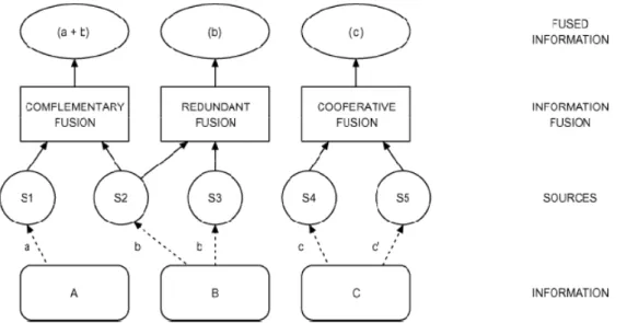
The information fusion techniques can be classified in three categories according to the sources: complementary, Redundant, and Cooperative. The relationship can be illustrated as the following figure [16]:

Then we describe the three types of information fusion [16]:

z Complementary. When information provided by the sources represents different portions of a broader scene, information fusion can be applied to obtain a piece of information that is more complete (broader).

z Redundant. If two or more independent sources provide the same piece of information, these pieces can be fused to increase the associated confidence.

z Cooperative. Two independent sources are cooperative when the information provided by them is fused into new information (usually more complex than the original data) that, from the application perspective, better represents the reality.

Fig. 1.1 Types of information fusion based on the relationship among the sources.

(15)

In this paper, we focus on the information fusion techniques applied in sensor network cooperating with intelligent systems. We begin with a brief review of information fusion method and algorithms which are able to applied in sensor networks.

1.1.1 Inference

z Bayesian Inference:

In the context of Bayesian inference, the information is represented in terms of conditional probabilities conditioned on the hypothesis we would like to infer and choose. The inference is based on the Bayes’ rule:

Pr | Pr | Pr

Pr 1.1 The posterior probability Pr | represents the “belief” of hypothesis Y given the information X. With the a prior probability Pr and conditional probability Pr | , we can derive the “belief” of the hypothesis when we have the information X and make inference according to the “belief.”

z Fuzzy Logic:

Fuzzy logic is concerned with the formal principles of approximate reasoning, with precise reasoning viewed as a limiting case. Fuzzy logic tries to model the imprecise modes of reasoning that play an essential role in the remarkable human ability to make rational decisions in an environment of uncertainty and imprecision. The following question is an example for the reasoning process that fuzzy logic aims to model.

“Most of those who live in Belvedere have high incomes. It is probable that Mary lives in Belvedere. What can be said about Mary’s income?”

The question involves many unspecific terms in natural language. Fuzzy

(16)

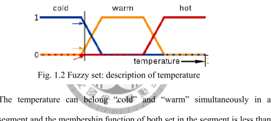
Fig. 1.2 Fuzzy set: description of temperature

logic theorem tries to establish a theoretical framework to deal with this kind of logic and reasoning.

Fuzzy set is the fundamental concept of fuzzy logic. It transforms the traditional set theory to fuzzy set by defining the membership function A,

: 0,1 1.2 which maps the members to values in [0,1] to represent its membership in the set. The membership can be some value between 0 and 1 to represent the ambiguity of the concepts or terms involved in the nature language. For example, the description of temperature can be fuzzy set which has the membership function as the following figure:

The temperature can belong “cold” and “warm” simultaneously in a segment and the membership function of both set in the segment is less than 1 to represent the ambiguity and uncertainty.

Based on the fuzzy set concept, the intersection and union operations, t-norm and t-conorm, is established. Then with the fuzzy set theory and operations, fuzzy relation and inference can be developed. The fuzzy inference in the form of conditional statement is widely applied in the information fusion problem in sensor network and will be discussed in detail in the succeeding section and chapter 4.

1.1.2 Estimation

z Maximum Likelihood (ML) and Maximum a posterior (MAP) estimation:

(17)

Estimation methods based on likelihood are suitable when the parameter being estimated is nonrandom. With the likelihood function

| 1.3 where is the observation vector and x is the parameter we want to estimate.

Then the ML estimation is done by maximizing the likelihood function:

arg max | 1.4 The MAP estimation aims at estimating a random variable with known probability . Based on Bayesian theory, we can convert the likelihood function | to the a posterior probability | with . Then we have the MAP estimation:

arg max | 1.5 z Kalman Filter:

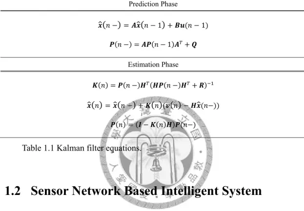
Kalman Filter is a well-known theory applied in various area including control system, tracking system and sensor network. Kalman filter is first appeared in R.E. Kalman’s famous paper in 1960 [44], in which describes a recursive solution to the discrete data linear filtering problem. The Kalman filter addresses the general problem of trying to estimate the state of a discrete-time controlled process that is governed by the linear stochastic difference equation:

1 1.6.1 1.6.2 The random vector and and represent the process and measurement noise respectively. In fact, the Kalman filter is a set of mathematical equations that provides an efficient computational (recursive) means to estimate the state of a process, in a way that minimizes the mean of the squared error [45].

(18)

The Kalman filter estimates a process by using a form of feedback control: the filter estimates the process state at some time and then obtains feedback in the form of (noisy) measurements. As such, the equations for the Kalman filter fall into two groups: time update equations and measurement update equations.

Prediction Phase

1 1

1 Estimation Phase

Table 1.1 Kalman filter equations.

1.2 Sensor Network Based Intelligent System

Originally, sensor network has been applied in various areas including environment monitoring, forest fire detection, military, drug administration…etc [46-48]. Recent technology advances have lead to the emergence of application of sensor network in various areas including robotic automation system [7,8], intelligent vehicle and transportation system [29,30], and even body area network for biomedical applications [24,49,50]. Most of these systems are operated by deploying the sensor network in the operation environment, such as roadside, buildings, or even inside human body, to monitor the environment and cooperate with intelligent devices, such as a robot or intelligent vehicle, which actively or passively collecting observations

(19)

from sensor network to perform their tasks. We call these systems Sensor Network Based Intelligent System (SNBIS) in this paper. In SNBISs, the intelligent devices rely on sensor network deployed in the environment to observe the physical world. By collecting the sensor observations, the intelligent device can perceive the environment and perform control actions to execute tasks. Consequently, in order to make correct inference from observations to execute the tasks accurately and efficiently, an intelligent decision framework, which is capable of effectively unified modeling the process from observations of the physical world to the executions of the tasks by the intelligent device, plays an extremely important role in this kind of systems.

There have been many researches on SNBISs already, especially the robot and vehicle being the intelligent devices [7,8,11], while the research on medical applications is emerging [24]. Common application scenarios are obstacle avoidance navigation for the robot [10], localization of robot by cooperative schemes [12], or crash avoidance for intelligent vehicle [30]. The research topics include data collection from network perspective [13], multiple access control [14], robot task allocation [15], and information fusion (or data fusion) to link the observation to the robot’s missions, which is the most essential part of the SNBIS. In works regarding this realm, information fusion algorithms [16] such as Kalman filter [20], occupancy grid [21], Baysian inference [19], fuzzy logic [18] are applied to deal with different problems. Many information fusion algorithms can be extended to apply in making decision on multiple kinds of sensor observation. There are also some researches devote in this kind of SNBIS. Most of them focus on heterogeneous sensors with different sensing quality [22,23,28] or fusing observations of different physical quantities by fuzzy logic instead of statistical inference [17].

Although tremendous research effort have devoted in subjects of information fusion or data aggregation in SNBIS, they all focus on specific part of the problem

(20)

instead of seeking for a general unified theoretical framework from sensor observation to task execution. Application specific works like the algorithms for robot navigation problem [11] is only suitable for small range of applications. The control approaches such as artificial potential field ignore the signal processing while concentrate on control actions corresponding to the environment like obstacle on the road [10,31]. The unified frameworks like Ubiquitous Robotic Space mostly deal with the cooperation among devices and availability of sensor network data to the intelligent devices [25,26]. Problems regarding sensor network monitoring tasks, intruder detection as example, focus on the signal processing but are lack of control action consideration corresponding to the detection event [27]. However, as the development of the intelligent device technology, more and more applications of complex missions in various environments utilizing SNBISs are emerging.

Consequently, an unified general theoretical framework from sensor observation to task execution, which is able to serve as a foundation to develop the algorithms and action mechanisms for various application scenarios of SNBIS, is necessary to realize the implementation of SNBIS in various environments. Moreover, this framework must enable the intelligent device to cooperate with various sensors observing different physical phenomenon in the same sensor network to execute the task more efficiently.

1.3 Organization

This paper is organized as follows. We establish the system model of SNBIS intelligent decision framework in Chapter 2. Chapter 3 follows to derive the solution of the application example, firefighting robot navigation problem, by the intelligent

(21)

decision framework. In Chapter 4, we extend the framework to multiple observation case. Many information fusion schemes including optimal fusion, Observation Selection, Ratio Combining, and Fuzzy Logic. The application example, firefighting robot, follows in Chapter 5. Chapter 6 presents the numerical and simulation results of the application examples of proposed approaches. The application of the intelligent decision framework in Cognitive Radio Spectrum Sensing is presented in Chapter 7.

Finally, the conclusion and future work is presented in Chapter 8.

(22)

Chapter 2 Intelligent Decision Framework

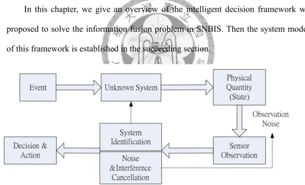
In this chapter, we give an overview of the intelligent decision framework we proposed to solve the information fusion problem in SNBIS. Then the system model of this framework is established in the succeeding section.

2.1 Framework Overview

In this paper, we develop a novel framework called intelligent decision framework.

Fig. 2.1 Intelligent decision making mechanism for sensor network based intelligent systems.

(23)

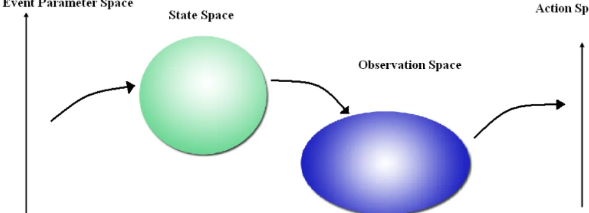
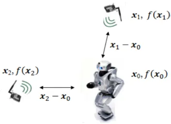
We derive intelligent decision framework by exploring the relationship between sensor observation and task execution to merge the processes, signal processing, decision, and control action, into a single framework. In SNBISs, the event related to the intelligent devices’ tasks induces the physical quantity variations in the environment and sensors are able to transfer the observations of these physical quantities to the intelligent devices to make decision and execute tasks (Fig. 2.1).

Thus we can model the sensor observation by two mappings, one from event (event parameter space) to physical quantity (state space) and one from physical quantity (state space) to observation (observation space). Then the intelligent device can make decision to execute tasks (action space) based on the above two mappings according to a cost function, which is the function of event and action. Unlike traditional approaches, these mappings in the framework cover the processes from sensor observation to control action and are applicable in various application scenarios. An example of sensor network navigation for firefighting robot problem (firefighting robot navigation problem in brief) follows to illustrate the application of this framework. The example also shows that the traditional decision scheme is just a degenerated case of our framework under special conditions. Then we extend this framework to intelligent decision framework for observations from multiple kinds of physical quantities. In multiple observation intelligent decision framework, the two mappings, event space to state space and state space to observation space, are extended to account for the variations of different physical quantities induced by the event and observation processes of different sensors. Consequently, we are able to simultaneously model the uncertainty and correlation among different physical quantities and different sensor observation precisions beyond traditional approaches.

Optimal decision scheme for multiple observations is developed as well as Observation Selection scheme, which ignores the complex correlation structure

(24)

among different physical quantities to make decision by limited knowledge of the nature. The condition for equivalence between Observation Selection and optimal decision is zero mutual information between the event and the observations other than selected one. To reduce the computation complexity, Observation Selection by Cramer-Rao bound is developed under specific conditions. In many multiple observation decision applications, fuzzy inference base on fuzzy conditional statement [2], a widely used fuzzy logic control approach, is applied to make decision with less strict-sense mathematic structures. We show that by Observation Selection, we can degenerate the decision scheme to the fuzzy logic controller under the strict mathematical structure of our intelligent decision framework. The example for multiple observation decision also follows up to illustrate the application of the framework and the fuzzy logic formulation.

2.2 System Model

In this section, we construct the system model of intelligent decision for the sensor network based intelligent system. In intelligent decision framework, we formally define and formulate the mathematical relationship between the essential elements involving in the decision process: event parameter, physical quantity related to the event (physical quantity in brief), sensor observation and the control action of the intelligent device. Traditional estimation problem in decision theory directly maps event to sensor observation. However, in order to derive a general framework unifying sensor observation aggregation, decision fusion and control action that is applicable to various environment, we reconstruct two mappings to account the uncertainty involve in the process. The process involves the uncertainty (or incomplete information) of the relationship between event parameter and physical

(25)

quantities and the uncertainty introduced during observation of the physical quantities (observation noise). According to this concept, we construct the framework of the intelligent decision as follows.

Definition 2-1.1: (Event Space) Event Space is composed of the event parameter, denoted by , representing the environmental facts or events that are necessary for the intelligent system to make the decision.

Definition 2-1.2: (Observation Space) Observation Space is composed of the quantity of observations, denoted by , from sensors.

Remark: The observations are the physical quantity plus noise and interference induced during sensor observation.

Definition 2-1.3: (State Space) State space is composed of the observable physical quantity induced by the events. We call them state and denoted by .

Definition 2-1.4: (Action space) Action space is composed of the decision of actions of the intelligent device, denoted by .

Definition 2-1.5: (Utility function) The utility function is the reward of the system receiving by making a decision on its action, denoted by ,

Fig. 2.2 Mathematical structure of intelligent decision making mechanism for sensor network based intelligent systems.

(26)

Remark: The utility function must reach its maximum value when the action matches the event parameter, and decrease when the action is more inconsistent with the event parameter. If the system should be panelized by each incorrect decision, we use cost function instead.

Definition 2-2: (Optimal decision mapping) The optimal decision mapping is the mapping Π: that maximize the utility function ,

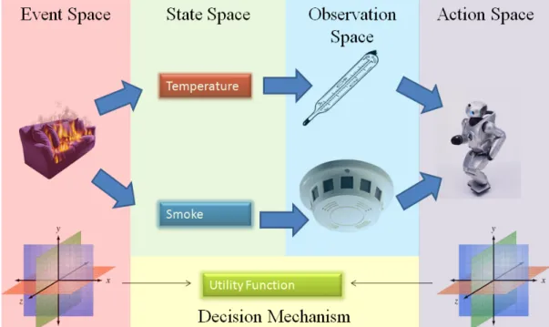
We use an example, sensor network navigation for firefighting robot (Fig.2.3), to illustrate the above definitions. The necessary information for firefighting robot’s task, reaching the place on fire, is the direction of the place on fire. Hence it is defined to be the event parameter. The fire induces abnormal temperature distribution (or smoke density) in the environment. Consequently, the temperature (smoke) is the physical quantity the sensors should observe. The temperature (smoke density) read on the sensor’s thermometer (smoke detector) is the observation aggregated by the firefighting robot. Finally, the control action is the robot’s movement direction decided by the sensor observations. Traditional estimation only estimates the exact value of the observed physical quantity considering the observation noise. Hence it can not directly determine the control action. However, our intelligent decision considers the relationship between event and the induced physical quantity and is able to determine the control action according to the utility function under the unified framework. We illustrate the decision mechanism by the mappings between the spaces as follows.

Proposition 2-3: The optimal decision mapping, Π: , is determined from the mapping from event space to state space, Φ: , and the mapping from state space to observation space, Ψ: , to maximize the utility function ,

(27)

Fig. 2.3 Sensor network navigation for firefighting robot under intelligent decision framework

Remark: From above discussion and definition, we know the state is induced by the event parameter by the mapping Ψ: . Noise and interference are introduced during sensor observation and establish the mapping Φ: . Consequently, we must use Ψ: and Φ: to construct the optimal decision mapping Π: to maximize the utility function , .

Generally speaking, Φ: involves noise and interference introduced during observation. It can be represented by conditional probability p | as traditional sensor estimation problem. For the mapping Ψ: , we have the following proposition:

Proposition 2-4: The mapping Ψ: can be represented by the conditional probability p |

Remark: The uncertainty of Ψ: comes from the uncertainty or incomplete

(28)

information of the relationship between the physical quantities we observe and the desired event. We call this “system model uncertainty,” or “model uncertainty” in brief. Unlike the mapping Φ: which depends on noise statistics, this mapping depends on the knowledge of the nature and is usually complex.

If this relationship is deterministic and completely known or state and event parameter is the same physical quantity, the mapping degenerates to deterministic or identical mapping. For example, when tracking a fighter, the relationship between the observable physical quantity (radar signal) and the event parameter (fighter’s position) is known, the mapping is deterministic. Besides this, with appropriate conditions, we can degenerate Ψ to the deterministic or identical mapping. For example, for firefighting robot navigation problem, the mapping from the direction towards fire (event parameter) to the direction of temperature gradient (state) is an identical mapping if the pattern of the potential field modeling the temperature distribution is radiative. This example will be discussed in detail in next section. For the mapping Ψ to be an identical mapping, we have the following corollary:

Corollary 2-5: Ψ is an identical mapping if and only if | 1

From above propositions, the mappings, Ψ: and Φ: , are represented by conditional probabilities. Hence we can interpret the optimal decision in Definition II-2 by the following proposition:

Proposition 2-6: (Optimal decision mapping) The optimal decision mapping, Π: , following Definition 2-2, is the mapping that maximize the a posterior expected utility function E , | .

(29)

Remark: The optimal decision on the action is the action that maximize the a posterior expected utility:

arg max E , | arg max , p | d 2.1

Baysian Inference

By applying Baysian theory, the a posterior probability p | becomes

p | p | p

p 2.2 p is the a prior distribution of the event. By Proposition 2-4 and the mapping Φ: , we can represent p | by the two conditional probabilities

p | p | p | d 2.3 And we apply (2.2) and (2.3) to (2.1), we have

arg max , p | p | d p

p d 2.4

arg max , p | p | p d d

,

2.5

(2.4) and (2.5) is equal because p is constant for every a. The two conditional probabilities, p | and p | , stands for the two mappings, Φ: and Ψ: , that involves in the decision mapping Π: . Consequently, the decision involves system identification for the modeling uncertainty p | as well as noise and interference cancellation for p | , as depicted in Fig. 2.1. We formulate insightful example of the firefighting robot navigation problem under the intelligent decision framework to demonstrate its application in next chapter.

(30)

Chapter 3 Sensor Network Navigation System for Firefighting Robot

In this chapter, we present the sensor network navigation system for firefighting robot problem, an application example of SNBIS, to show the effectiveness of the intelligent decision framework. This example has been investigated in [5]. But we reinvestigate it with the new framework proposed in this paper.

There is a firefighting robot making its way to the place on fire guided by the

Fig. 3.1 Scenario of Sensor Network Navigation System for Firefighting Robot

(31)

sensor network deployed in the environment. The sensors are the thermometers measuring the temperature. The robot collects sensor information (temperature) in this way: it collects the observations from nearby sensor around it and makes decision on movement direction by the observation from sensors and itself. Then the robot walks along the direction until it encounters another group of sensors around it and repeats this action until it reaches the place on fire. The firefighting robot is not equipped with the positioning system. Hence it does not know the precise information of location and direction of reference coordinate system.

3.1 Intelligent Decision Framework for Firefighting Robot

We formulate the decision problem of navigation system for firefighting robot under the intelligent decision framework. We model the temperature distribution induced by the fire as a potential field , . To simplify the problem, we consider the static potential field , that is, ignoring the time variance. In such kind of problems, the intelligent devices are usually lack the information about the nature system .

Following Definition 2-1.1~1.5 and the remarks, we define the event parameter as the direction of the fire, the observations as the temperatures observed by sensors and the action as the robot’s movement direction. The physical quantities (states) are defined to be the direction of highest temperature, namely, the gradient of the potential field, to represent the temperature distribution. The correspondence of spaces in the intelligent decision framework and sensor network navigation for firefighting robot is summarized in Table.3.1. Note that the robot does not know the

(32)

direction of reference coordinate system. Consequently, the above definitions are using the robot’s own coordinate system. Because the robot’s goal is to reach the place on fire, we define the utility function to represent how the robot is approaching the place on fire by each decision. Then the utility function is:

u , cos Arg Arg 3.1 Arg(α) is the angle with x axis of vector α, a is the robot’s movement direction (action), and is the direction of the place on fire (event parameter). We assume the length of robot movement between two successive sensor observation collections is unit length. Hence the utility function is proportional to the variance of the distance between the robot and the fire. Putting (3.1) into (2.5), the optimal decision of action

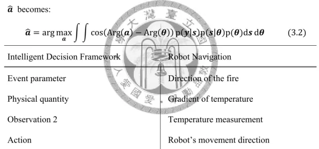
becomes:

arg max cos Arg Arg p | p | p d d 3.2 Intelligent Decision Framework Robot Navigation

Event parameter Direction of the fire Physical quantity Gradient of temperature

Observation 2 Temperature measurement

Action Robot’s movement direction

Table 3.1 Correspondence of Intelligent decision framework and robot navigation problem

3.2 Sensor Observation Model

We next establish the mapping Φ: by constructing the observation model.

We begin by defining the observation more precisely. The observation is defined to be the difference between the observed temperature from the sensors around the robot and from the robot itself. The sensor is able to observe plus noise, is the

(33)

location of the sensor, and robot itself can observe plus noise in its location , thus the potential difference, , plus noise is also observable.

Hence the relationship between the observations and states can be established approximately by the aid of Taylor Expansion. The Taylor Expansion of the potential field of a sensor in is:

∂

∂ … ∂

∂

, . . ,

! … ! …

∞

3.3 where

… , …

and the potential difference between the robot and the sensor is

∂

∂ … ∂

∂

, … ,

! … ! …

∞

3.4 Assume the dimension d=2. If we approximate the potential difference by the linear term, and note that the relationship between the gradient and the differentiation of the field is

′ | ∂

∂ d ∂

∂ d ^T· 3.5 where

d d

With Taylor expansion (3.4), when the difference between two location vectors, and , is sufficiently small, we are able to approximate the potential field difference

(34)

Fig. 3.2 Sensor observation model by the first order term:

∂

∂ ^T· 3.6

Then we can establish the sensor observation model related to the gradient (state):

′ |

′ |…

T

… T · 3.7

n is the difference of observation noise of the sensors and the robot. The robot can infer the gradient (state) by this observation model. By this approximation model and the distribution of n, we can derive the conditional distribution p | where

. Then if we can specify the mapping Ψ: , we can derive the optimal decision mapping Π: . Generally speaking, this mapping is usually hard to derive directly due to the insufficient information of the unknown system. However, if Ψ: is an identical mapping, this problem will reduce to traditional estimation problem in the form of state space model. We derive the degenerate form of state space model in the following.

(35)

3.3 Degenerate Problem: State space model

Now we investigate the conditions for the intelligent decision problem of the firefighting robot to degenerate to the traditional state space estimation problem.

When the mapping Ψ: is an identical mapping, we are able to estimate the event parameter by estimating the state through (3.7), which will be proved in the following. And we can formulate the state space model based on observation model (3.7). Consequently, to degenerate this problem to the traditional form, we must find out the condition for Ψ to be an identical mapping.

We start by investigating , which generates the mapping Ψ. When we have precise knowledge of and robot’s location x, the relationship between state s (gradient of the potential field) and event parameter should be a deterministic function:

, 3.8 , can be determined by . However, we assume unknown and no available location information. Consequently, we model their relationship by conditional probability p | according to Proposition 2-4. However, the mapping reduces to an identical mapping under appropriate conditions. If we know satisfies the following condition,

c ,

for all , and is an arbitrary scalar function of 3.9 we have

p Arg Arg | 1 (3.10) (3-10) is equivalent to p | 1 when we consider the expected a posterior utility E cos Arg Arg | . There are many kinds of potential field

(36)

satisfying this condition, including electrostatic field and diffusion in free space [6].

As long as the temperature distribution could be modeled by these kinds of potential fields, this condition holds. Then following the concept of Corollary 2-5, we can formally prove that the optimal decision mapping can be constructed by estimating state under condition (3.9).

Corollary 3-1: Estimating state (gradient of potential field) is equivalent to estimating event parameter in the sense of utility function (3.1) if (3.9) (or equivalent, (3.10)) holds.

Proof:

We need to prove that under the condition (3.10), we have arg max

′ E cos Arg ′ Arg | arg max E cos Arg Arg |

As mentioned above, p | 1 is equivalent to (3.10) when calculating E cos Arg Arg | . Hence we use p | 1 instead.

The estimation of gradient is arg max

′ E cos Arg ^′ Arg | arg max

′ cos Arg ^′ Arg p | p d 3.11 The maximum expectation of utility function is

max E u ,

max E cos Arg Arg | 3.12

max cos Arg Arg p | p | p d d 3.13 max cos Arg Arg p | p d 3.14 The equality of (3.13) and (3.14) holds because p | 1 and thus

(37)

p | 0 Hence

arg max cos Arg Arg p | p d 3.15 according to (3.11). Then the Corollary is proved. Q.E.D

Corollary 3.1 shows that under the condition (3.9) on the potential field, the observed physical quantity is identical to the event parameter for the utility function (3.1). Consequently, we are able to use the linear approximation observation model (3.7) to estimate the physical quantity (state) to make action decision without considering event parameter.

In addition to the observation model, we proceed to derive the state transition and formulate the problem into the state space estimation problem. We observe that the gradient is always point to wherever the robot stands on. Hence it is always the same when the robot makes right direction decisions, and would not change significantly even when it makes wrong direction decisions due to the small displacement between two observation collections assumed in the observation model.

Recall that the state is defined to be the direction of the destination in robot’s own coordinate system and this relative coordinate would rotate when the robot turns its direction, or say makes wrong decision. Hence change of the gradient’s direction comes mostly from the relative coordinate rotation instead of the gradient’s direction rotation in absolute coordination system when the robot makes wrong decision. We can conclude from above observations that the direction of gradient in the robot’s own coordinate system is the difference between in the direction of estimated gradient and the true gradient. Then the state transition is:

3.16

(38)

u is a random variable accounts for the direction deviation of the robot’s movement due to obstacles, mechanical errors or other non-ideal effects. Here we use normalized gradient to represent its direction. is the position vector of n’th observation.

The similar navigation problem has been investigated in [5] in a simplified version. We generalized the discrete direction selection solved by Maximum a posterior (MAP) hypothesis testing to the continuous vector form (3.17) and relieve the unrealistic assumptions on the observation model to derive the linear approximate observation model (3.7). Then the firefighting robot navigation problem can be formulated by modified state-space model with the estimation of previous state in state transition:

(3.17.a) (3.17.b)

where

T

…T , is also measured in the robot’s own coordinate

system.

Then we can adapt the widely used MMSE method, Kalman filter, to solve it. In order to apply Kalman filter, we should make a further assumption to limit the error is in a small range in which the approximation

cos arg arg ~1 | | 3.18 holds. The assumption assures Kalman filter to fit the optimal decision mapping to maximize the utility function because it makes MMSE decision. However, (3.17.a) and (3.17.b) is different from traditional state-space model of Kalman filter problem due to the additional term, estimation of previous state, in (3.17.a). In fact, in many papers, for example [32], the estimation of previous state has been applied in the prediction problem. In [5], we solve this problem by directly applying MAP hypothesis testing due to the discrete direction form. But when we generalize it to

(39)

continuous direction, we should solve it by modifying solution of Kalman filter.

However, it turns out that the estimation of previous state can be regard as outside input in solving Kalman filter. We prove this in the Lemma A1 in Appendix 3. Then with this lemma, we can solve the state space model by Kalman filter approach. The solution is:

Prediction Phase

(3.19) (3.20) Estimation Phase

T T T (3.21)

(3.22) (3.23) Table. 3.2 Kalman filter

where

E ^T , E ^T

We can use above equations to recursively solve our state space model estimation problem.

Appendix 3.A State-space Model with Estimation of Previous State

In Section 3.3, we derive the state space model of the firefighting robot navigation problem. The state space model (3.17.a), (3.17.b) is different from state space model of Kalman filter due to that it includes the estimation of previous state in

(40)

state transition equation. However, in this section we show that the estimation of previous state in state transition equation can be regarded as outside input in Kalman filter when deriving the LMMSE state estimation.

Lemma 3.A1: The estimation of previous state in state transition equation of state-space model is the same as outside input in the state transition equation of Kalman filter when solving the LMMSE state estimation problem.

Proof:

The state-space model including the estimation of previous state can be formulated as:

n n, n 1 n 1 n, n 1 n 1 n (3.24) n n n n (3.25) E n s ′ n δ (3.26) E n s ′ n δ (3.27) where n 1 is the estimation of previous state n 1 .

Based on the innovation process concept in [1], we can derive the LMMSE of n ’s as follows:

Define the innovation process:

n n n n|n 1 (3.28) And the covariance of estimation of n n

n E n n|n 1 n n|n 1 ′ (3.29)

n n n (3.30) We use E to denote the ensemble average. And we require

s n n for s n (3.31) By projection theory

n E n ^′ k k k k 3.32

(41)

E n ^′ k k k k

E n ^′ n n n n 3.33

n n E n, n 1 n 1 n, n 1 n 1

n ^′ k k k k 3.34

n n n, n 1 n 1

n, n 1 E n 1 ^′ k k k k 3.35

In (3.34), we define

n E n ^′ n n n

and in (3.35), we use that fact that

n, n 1 n 1 n, n 1 E n 1 ^′ k k k k

(3.36) The first two terms in RHS is the same as derivation in [1]. Then we deal with the last term:

E n 1 ^′ k k k k 3.37

E n 1 n 1 n 1 ^′ k k k k 3.38

Because n 1 n 1 is orthogonal to ^′ k according to (3.31), we have

E n 1 ^′ k k k k 3.39

(42)

E n 1 ^′ k k k k 3.40

n 1 (3.41) Put (3.41) into (3.35), we have

n E k ^′ k k k k

n n n, n 1 n 1 n, n 1 n 1 3.42 The original solution of Kalman filter based on innovation process is

n n n n, n 1 n|n 1 3.43 From (3.42), we can observe that n, n 1 n 1 can be directly added, without alternating the terms in the original form (3.43), to the estimation like an outside deterministic input to the state transition system. Consequently, we know that the estimation of previous state can be regarded as outside input to the system and ordinary algorithm solving state-space model of Kalman filter is able to solve the state space model with estimation of previous state without any modification.

Q.E.D

(43)

Chapter 4 Intelligent Decision Framework- Multiple Observation

In previous sections, the intelligent decision framework fuses observations of single kind of physical quantity. However, in many application scenarios of sensor network based intelligent systems, multiple kinds of physical quantities may change in response to the occurrence of an event. For example, fire can induce high temperature and heavy smoke intensity, or even the number of broken sensors can be taken as observations. Intuitively, efficiently taking the observations of more kinds of

Fig. 4.1 Intelligent decision making mechanism with multi-observation for sensor network based intelligent systems (detail of decision block omitted).

(44)

(a) (b)

Fig. 4.2 Comparison of (a) multiple observation intelligent decision framework and (b) traditional multiple observation model

physical quantities into consideration in decision process may improve the system performance. Traditional estimation schemes, which directly map event to observation, are only able to solve the fusion problem of observations of the same physical quantity from sensors with different precisions [23,28]. However, our intelligent decision framework separates the mappings and are able to simultaneously model the uncertain and correlation of different physical quantities and uncertain introduced by different sensor precisions. We formulate the multi-observation intelligent decision by extending the framework in Chapter 2 in the following.

4.1 Optimal Multi-Observation Decision System Model

Extending the framework established in section II, we have the following definitions:

Definition 4-1.1: (Observation space) Observation space is defined to be the Cartesian product of the observation spaces of each kind of observations.

Remark: Different sensors collect different kinds of observations simultaneously.

(45)

Con corr spac is th the

Def the Rem Con

The deci mul

mul

Fig nsequently,

responding ce of multi- he number sub-observa

finition 4-1.

state spaces mark: Differ nsequently,

e definition ision, and lti-observati

We again ltiple kinds

g. 4.3 Intelli the observa to each kin -observation of kinds o ation spaces

2: (State sp s correspon rent kinds o

of event s also deno ion decision n use the f of observat

igent Decis ation space i

nd of senso n decision p f observatio s.

pace) State nding to eac of observati

… . .

space and a oted by n.

firefighting tions to elu

ion framew is the Carte ors. Accord problem bec

ons. We ca

space is de ch kind of ph ions are rais

.

action space and .

robot nav ucidate the a

work : multip sian produc ding to the d

comes all the

efined to be hysical quan sed from di

e are the sa Then we

vigation sce above defin

ple observat ct of the obs definition, t

observation

e the Carte ntities.

fferent phy

ame as sing can defin

enario of C nitions. The

tion

servation sp the observa

… . . n space and

esian produc

sical quanti

gle observa ne the opt

Chapter 3 fire can ind

paces ation , K d

ct of

ities.

ation timal

with duce

(46)

heavy smoke and high temperature in the environment. If there are two kinds of sensors, thermometer and the smoke detector, in the environment, the firefighting robot is able to collect two kinds of observations, temperature and smoke density.

Then observation space is consist of temperature observations, observation space is consist of smoke density observations, and the observation space for decision is . Similarly, is temperature and is smoke density.

The event parameter and action is the same as single observation case. Based on above definitions, we have the definition of optimal multi-observation decision:

Definition 4-2: (Optimal multi-observation decision) The optimal multi-observation decision mapping is the mapping Π: that maximize the a posterior expected utility function E , | , , … ,

We expand the a posterior expected utility function E , | , , … ,

, p | , , … , d

, … p , , … , | , , … , p , , … , | d … d

, ,…, p d

(4.1) And the decision mapping is decided by maximizing (4.1)

max E , | , , … ,

max , … p , , … , | , , … , p , , … , | d … d

, ,…, p d

max , … p | p , , … , | d … d

, ,…,

p d

(4.2)

(47)

In (4.2), we assume p , , … , | , , … ,

p | , , … , p | 4.3

which means that given the states, the observation of each state is independent, and the observations are independent with other states excepted the corresponding state.

Hence the mapping Φ: can be separated in to independent mappings Φ : . This is quite reasonable because each sensor observes each physical quantity (state) independently and would not be affected by other states. However, although it is reasonable to assume the independence of the conditional probability p | ’s, the independence among physical quantities given the event parameter does not hold in general. For example, in the scene of fire, the place with high temperature will have high smoke density with high probability. Generally speaking, the physical quantities changed by the same event are highly correlated and the correlation is too complex to derive directly. Hence, we develop the “Observation Selection”, a decision mapping to optimally select one observation to make decision without considering the correlations among the physical quantities.

4.2 Observation Selection

In order to avoid dealing with the correlations among the different physical quantities, Observation Selection scheme selects the best observation according to the utility function and makes decision by this selected observation. In Observation Selection, we reduce the general optimal decision of multi-observation problem into selection of a best observation among all kinds of observations to make decision.

(48)

(Fig.4.4) We first define the sub-decision mapping:

Definition 4-3: (Sub-decision mapping) The sub-decision mappings are defined to be the mapping from each sub-observation space to action space that maximize the a posterior expected utility function E , | .

We denote the sub-decision mapping by

Π :

Then the expected a posterior utility E for sub-decision mapping Π is

E , | , p | p | p d d 4.4 And the mapping Π is decided by

max E , | 4.5 (4.4) is the same as the single observation expected a posterior utility except the observation indices. The mapping considered here is and instead

of and .

Sub-decision mapping divides the observation space into individual observations and makes decision by those sub-observation spaces separately. Observation Selection is the decision scheme to select the best sub-decision mappings. Following the definition of sub-decision mapping, we formally define Observation Selection as follows:

Definition 4-4: (Observation Selection) Observation Selection is the decision mapping that has the largest a posterior expected utility function among all Π , 1, … , Then the optimal decision mapping Π of Observation Selection is:

arg max max E , |

Π Π 4.6

(49)

Fig. 4.4 Comparison of optimal decision and Observation Selection Expanding the maximum expected a posterior utility, we have

max max E , |

max max , p | p | p d d 4.7 When applying Observation Selection, instead of combing all observations and fusing them to make decision, we select the “best” observation to make decision due to lack of the information regarding correlations among states. For example, the firefighting robot using Observation Selection first chooses among the observations from thermometer and smoke detector then makes decision by the selected observations.

We next investigate under what conditions the Observation Selection being equivalent to the optimal decision mapping. Denote the index of the sub-decision mapping that has the largest maximum expected a posterior utility by . Intuitively, if the observations other than the selected one do not provide information when making the decision, the Observation Selection is optimal. In other words, the conditional mutual information of event parameter and the observations other than the

(50)

selected one given the state of the selected observation, I , … , , … , ; | , is zero. In order to prove that conditional mutual information being zero is the sufficient and necessary condition for optimality of Observation Selection, we prove the following lemma first:

Lemma 4-5. I , … , , … , ; | 0 is equivalent to

p , … , , … , | , being const with respect to and . Proof:

I , … , , … , ; |

p , … , , … , , , log p , … , , … , , |

p , … , , … , | p |

,…, , …, , ,

0 4.8 Hence

p , … , , … , , |

p , … , , … , | p |

p , … , , … , | ,

p , … , , … , | 1 4.9 Then

p , … , , … , | ,

p , … , , … , | 4.10 p , … , , … , 4.11 (4.10) is due to (4.9). (4.11) holds because the observations depend only on its corresponding state and is independent of other states. p , … , , … , is a constant with respect to and .

Q.E.D We proceed to prove that I , … , , … , ; | 0 is the sufficient and necessary condition for optimality of Observation Selection in the following theorem:

Theorem 4-6 Observation Selection is equivalent to optimal decision mapping if and

(51)

only if I , … , , … , ; | 0 Proof:

From Lemma 4-5, we know that if I , … , , … , ; | 0, then

p , … , , … , | ,

… p |

,

· p , … , , … , | , d … d d … d

(4.12) is a constant with respect to and . We first prove the “if” part and then the “only if” part.

1. “if” part

The a posterior utility of optimal decision mapping is max E , | , , … ,

max , … p | p , , … , | d … d

, ,…,

p d

(4.13)

… p | p , , … , | d … d

, ,…,

p | p | … p |

,

p , , … , |

p | d … d d … d d

(4.14) p , , … , |

p | p , … , , … , | , 4.15 Hence if

… p |

,

· p , … , , … , | , d … d d … d

is a constant, denoted by c, with respect to and , then put (4.15) into (4.14), we have

(52)

… p | p , , … , | d … d

, ,…,

p | p | · d 4.16 and by put (4.16) into (4.13), the a posterior utility of optimal decision mapping becomes

max , p | p | · d p d

max , p | p | d p d

,

4.17

max , p | p | d p d 4.18

(4.18) is identical to the maximum a posterior probability of Observation Selection in (4.7). Hence we have proved that the two decision mappings are equal.

2. “only if” part E , | , , … ,

max , … p | p , , … , | d … d

, ,…,

p d

max , p | p | d p d

,

4.19

Because the equation is true for any utility function ,

… p | p , , … , | d … d

, ,…,

p | p | · d 4.20 Differentiate with respect to , we have

· p | p |

(53)

p | p | … p |

,

· p , … , , … , | , d … d d … d

4.21 c is constant with respect to because the terms in (4.20) except c are function of

’s. Consequently, c is not a function of . Hence

… p |

,

· p , … , , … , | , d … d d … d

is constant. Q.E.D

Theorem 4-6 is an intuitive result of the concept of mutual information. Mutual information I(X;Y) is the reduction in the uncertainty of X due to the knowledge of Y (or uncertainty reduction of Y due to knowledge of X). Hence Observation Selection is optimal when the knowledge of the observations except the selected one are not able to reduce the uncertainty of the event parameter given the state of the selected observation. Zero mutual information also implies the independence of the two random variables. Hence we also know the optimality condition of Observation Selection can also be stated as the event parameter conditioned on the selected state is independent of the other observations.

4.3 Cramer-Rao bound

Although we can avoid dealing with the complex correlation structure between the states by Observation Selection scheme, the selection rule (4.6) is still tedious. We