Clustering Complex Data with Group-Dependent Feature Selection
Yen-Yu Lin1,2, Tyng-Luh Liu1, and Chiou-Shann Fuh2
1Institute of Information Science, Academia Sinica, Taipei, Taiwan
2Department of CSIE, National Taiwan University, Taipei, Taiwan {yylin,liutyng}@iis.sinica.edu.tw [email protected]
Abstract. We describe a clustering approach with the emphasis on de- tecting coherent structures in a complex dataset, and illustrate its effec- tiveness with computer vision applications. By complex data, we mean that the attribute variations among the data are too extensive such that clustering based on a single feature representation/descriptor is insuffi- cient to faithfully divide the data into meaningful groups. The proposed method thus assumes the data are represented with various feature rep- resentations, and aims to uncover the underlying cluster structure. To that end, we associate each cluster with a boosting classifier derived from multiple kernel learning, and apply the cluster-specific classifier to feature selection across various descriptors to best separate data of the cluster from the rest. Specifically, we integrate the multiple, correlative training tasks of the cluster-specific classifiers into the clustering procedure, and cast them as a joint constrained optimization problem. Through the op- timization iterations, the cluster structure is gradually revealed by these classifiers, while their discriminant power to capture similar data would be progressively improved owing to better data labeling.
1 Introduction
Clustering is a technique to partition the data into groups so that similar (or coherent) objects and their properties can be readily identified and exploited.
While such a goal is explicit and clear, the notion of similarity is often not well defined, partly due to the lack of a universally applicable similarity measure.
As a result, previous research efforts on developing clustering algorithms mostly focus on dealing with different scenarios or specific applications. In the field of vision research, performing data clustering is essential in addressing various tasks such as object categorization [1, 2] or image segmentation [3, 4]. Despite the great applicability, a fundamental difficulty hindering the advance of clustering techniques is that the intrinsic cluster structure is not evidently revealed in the feature representation of complex data. Namely, the resulting similarities among data points do not faithfully reflect their true relationships.
We are thus motivated to consider establishing a clustering framework with the flexibility of allowing the data to be characterized by multiple descriptors.
The generalization aims to bridge the gap between the resulting data similari- ties and their underlying relationships. Take, for example, the images shown in
Fig. 1.Images from three different categories: sunset, bicycle and jaguar
Fig. 1. Without any ambiguities, one can easily divide them into three clusters.
Nevertheless, say, in an object recognition system, color related features are re- quired to separate the images in category sunset from the others. Analogously, shape and texture based features are respectively needed for describing cate- gories bicycle and jaguar. This example not only illustrates the importance of using multiple features but also points out that the optimal features for ensuring each cluster coherent often vary from cluster to cluster.
The other concept critical to our approach is unsupervised feature selection. It is challenging due to the absence of data labels to guide the relevance search, e.g., [5, 6]. To take account of the use of multiple descriptors for clustering, our formu- lation generalizes unsupervised feature selection to its cluster/group-dependent and cross feature space extensions. To that end, each cluster is associated with a classifier learned with multiple kernels to give a good separation between data inside and outside the cluster, and data are dynamically assigned to appropri- ate clusters through the progressive learning processes of these cluster-specific classifiers. Iteratively, the learned classifiers are expected to facilitate the reveal- ing of the intrinsic cluster structure, while the progressively improved clustering results would provide more reliable data labels in learning the classifiers.
Specifically, we integrate the multiple, correlative training processes of the cluster-specific classifiers into the clustering procedure, and realize the unified formulation by 1) proposing a general constrained optimization problem that can accommodate both fully unlabeled and partially labeled datasets; and 2) implementing multiple kernel learning [7] in a boosting way to construct the cluster-specific classifiers. Prior knowledge can thus be conveniently exploited in choosing a proper set of visual features of diverse forms to more precisely depict the data. Indeed our approach provides a new perspective of applying multiple kernel learning, which typically addresses supervised applications, to both unsupervised and semisupervised ones. Such a generalization is novel in the field. Different from other existing clustering techniques, our method can not only achieve better clustering results but also have access to the information regarding the commonly shared features in each cluster.
2 Related Work
Techniques on clustering can vary considerably in many aspects, including as- suming particular principles for data grouping, making different assumptions
about cluster shapes or structures, and using various optimization techniques for problem solving. Such variations however do not devalue the importance of clustering being a fundamental tool for unsupervised learning. Instead, cluster- ing methods such as k-means, spectral clustering [3, 8], mean shift [4] or affinity propagation [9] are constantly applied in more effectively solving a broad range of computer vision problems.
Although most clustering algorithms are developed with theoretic support, their performances still depend critically on the feature representation of data.
Previous approaches, e.g., [5, 6], concerning the limitation have thus suggested to perform clustering and feature selection simultaneously such that relevant features are emphasized. Due to the inherent difficulty of unsupervised feature selection, methods of this category often proceed in an iterative manner, namely, the steps of feature selection and clustering are carried out alternately.
Feature selection can also be done cluster-wise, say, by imposing the Gaus- sian mixture modelson the data distribution, or by learning a distance function for each cluster via re-weighting feature dimensions such as the formulations described in [10, 11]. However, these methods typically assume that the under- lying data are in a single feature space and in form of vectors. The restriction may reduce the overall effectiveness when the data of interest can be more pre- cisely characterized by considering multiple descriptors and diverse forms, e.g., bag-of-features [12, 13] or pyramids [14, 15].
Xu et al. [16] instead consider the large margin principle for measuring how good a data partitioning is. Their method first maps the data into the kernel- induced space, and seeks the data labeling (clustering) with which the maximum margin can be obtained by applying SVMs to the then labeled data. Subse- quently, Zhao et al. [17] introduce a cutting-plane algorithm to generalize the framework of maximum margin clustering from binary-class to multi-class.
The technique of cluster ensembles by Strehl and Ghosh [18] is most relevant to our approach. It provides a useful mechanism for combining multiple cluster- ing results. The ensemble partitioning is optimized such that it shares as much information with each of the elementary ones as possible. Fred and Jain [19]
introduce the concept of evidence accumulation to merge various clusterings to a single one via a voting scheme. These methods generally achieve better clus- tering performances. Implicitly, they also provide a way for clustering data with multiple feature representations: One could generate an elementary clustering result for each data representation, and combine them into an ensemble one.
However, the obtained partitioning is optimized in a global fashion, neglecting that the optimal features are often cluster-dependent.
Finally, it is possible to overcome the unsupervised nature of clustering by incorporating a small amount of labeled data in the procedure so that satisfac- tory results can be achieved, especially in complex tasks. For example, Xing et al. [20] impose side information for metric learning to facilitate clustering, while Tuzel et al. [2] utilize pairwise constraints to perform semisupervised clustering in a kernel-induced feature space.
3 Problem Definition
We formalize and justify the proposed clustering technique in this section. Prior to that, we need to specify the notations adopted in the formulation.
3.1 Notations
Given a dataset D = {xi}Ni=1, our goal is to partition D into C clusters. We shall use a partition matrix, Y = [yic] ∈ {0, 1}N×C, to represent the clustering result, where yic = 1 indicates that xi belongs to the cth cluster, otherwise yic = 0.
Besides, let yi,: and y:,c denote the ith row and cth column of Y respectively.
To tackle complex clustering tasks, we consider the use of multiple descriptors to more precisely characterize the data. These descriptors may result in diverse forms of feature representations, such as vectors [21], bags of features [22], or pyramids [14]. To avoid directly working with these varieties, we adopt a strategy similar to that in [15, 23], where kernel matrices are used to provide a uniform representation for data under various descriptors. Specifically, suppose M kinds of descriptors are employed to depict each sample, i.e., xi = {xi,m ∈ Xm}Mm=1. For each descriptor m, a non-negative distance function dm : Xm× Xm→ R is associated. The corresponding kernel matrix Kmand kernel function kmcan be established by
Km(i, j) = km(xi, xj) = exp (−γmd2m(xi,m, xj,m)), (1) where γm is a positive constant. By applying the procedure to each descriptor, a kernel bank Ω of size M is obtained, i.e., Ω = {Km}Mm=1. The kernel bank will serve as the information bottleneck in the sense that data access is restricted to referencing only the M kernels. This way our method can conveniently work with various descriptors without worrying about their diversities.
3.2 Formulation
The idea of improving clustering performances for complex data is motivated by the observation that the optimal features for grouping are often cluster- dependent. Our formulation associates each cluster with a classifier to best inter- pret the relationships among data and the cluster. Specifically, a cluster-specific classifier is designed to divide the data so that its members would share cer- tain common features, which are generally distinct from the rest. Furthermore, the goodness of the clustering quality about a resulting cluster can be explicitly measured by the induced loss (namely, the degree of difficulty) in learning the specific classifier. It follows that the proposed clustering seeks an optimal data partitioning with the minimal total loss in jointly learning all the C cluster- specific classifiers.
As one may notice that our discussion so far would lead to a cause-and-effect dilemma: While the data labels are required in learning the cluster-specific clas- sifiers, they in turn can only be determined through the clustering results implied
by these classifiers. We resolve this difficulty by incorporating the learning pro- cesses of the cluster-specific classifiers into the clustering procedure, and cast the task as the following constrained optimization problem:
min
Y,{fc}Cc=1
XC c=1
Loss(fc, {xi, yic}Ni=1) (2)
subject to Y ∈ {0, 1}N×C, (3)
yi,:eC= 1, for i = 1, 2, ..., N, (4) ℓ ≤ e⊤Ny:,c≤ u, for c = 1, 2, ..., C, (5) yi,:= yj,:, if (i, j) ∈ S, (6) yi,:6= yj,:, if (i, j) ∈ S′, (7) where {fc}Cc=1are the cluster-specific classifiers. eC and eN are column vectors, whose elements are all one, of dimensions C and N respectively.
We now give justifications for the above constrained optimization problem.
Our discussions focus first on the part of constraints. With (3) and (4), Y is guaranteed to be a valid partition matrix. Since in practical applications most clusters are rarely of extreme sizes, we impose the desired upper bound u and lower bound ℓ of the cluster size in (5). The remaining constraints (6) and (7) are optional so that our method can be extended to address semisupervised learning. In that case, (6) and (7) would provide a set of pairwise instance-level constraints, each of which specifies either a pair of data points must reside in the same cluster or not. S in (6) and S′ in (7) are respectively used to denote the collections of these must-links and cannot-links.
Assuming that all the constraints are satisfied, the formulation would look for optimal data partitioning Y∗ such that, according to (2), the total induced loss of all the cluster-specific classifiers is minimized. That is, the proposed clustering approach would prefer that data residing in each cluster are well separated from the rest by the cluster-specific classifier (and hence yields a small loss), which is derived by coupling a discriminant function with an optimal feature selection to achieve the desired property. This implies that most of the data in an arbitrary cluster c would share some coherent characteristics implicitly defined by the optimal feature selection in forming fc∗. The proposed optimization elegantly connects the unsupervised clustering procedure with the supervised learning of the specific classifiers. By jointly addressing the two tasks, our method can uncover a reasonable cluster structure even for a complex dataset.
4 Optimization Procedure
To deal with the cause-and-effect factor in (2), we consider an iterative strategy to solve the constrained optimization problem. At each iteration, the cluster- specific classifiers {fc}Cc=1and the partition matrix Y are alternately optimized.
More specifically, {fc} are first optimized while Y is fixed, and then their roles are switched. The iterations are repeated until the loss cannot be further reduced.
4.1 On learning cluster-specific classifiers
Notice that in the constrained optimization problem (2) the cluster-specific clas- sifiers {fc} only appear in the objective function, and there is no correlation among them once Y is fixed. Thus, these classifiers can be optimized indepen- dently by minimizing their corresponding loss function. That is, fccan be derived by considering only the binary labeled data {xi, yic}Ni=1.
Our choice of selecting a suitable supervised learning methodology for con- structing the classifiers is based on two key requirements stemming from the properties related to the classifiers and the iterative training process. First, the cluster-specific classifiers should be generated by using information from mul- tiple kernels, i.e., via multiple kernel learning [7]. Second, the degree of data fitting in the classifiers can be conveniently controlled. The latter requirement arises due to the expected phenomenon that the data labels {yic}Ni=1 would be noisy during the earlier iterations, and then progressively become more accurate through the iterative optimization. By addressing this effect, we can significantly alleviate the possibility of overfitting or underfitting in learning the classifiers.
Having taken the two into account, we consider each fc a boosting classifier. In what follows, we describe the two main elements in learning such classifiers.
The pool of weak learners We adopt a similar strategy proposed in [24].
To begin with, the discriminant power of each kernel is transferred into a set of weak learners, called dyadic hypercuts [25]. We then construct the pool of weak learners by including the dyadic hypercuts generated from all the kernels in Ω.
The procedure naturally enables a boosting algorithm to learn classifiers that inherit the discriminant power from the multiple kernels.
A dyadic hypercut h is specified by three parameters: a positive sample xp, a negative sample xn, and a kernel function km. (Note that the positive and negative samples here depend on labels {yic}Ni=1.) The model for prediction is
h(x) = a · sign(km(xp, x) − km(xn, x) − θ) + b, (8) where a and b are real values, and θ is used for thresholding. The size of the set of weak learners is |H| = N+× N−× M , where N+ (N−) is the number of positive (negative) training data, and M is the number of kernels.
Loss function for boosting Among the many choices of loss function for learn- ing boosting classifiers, we have implemented two of the most popular ones, i.e., ExpLoss and LogLoss [26, 27], to test our method. In our experiments, LogLoss leads to better performances, and is thus adopted. It follows that in (2) we have
Loss(fc, {xi, yic}Ni=1) = XN
i=1
ln (1 + exp (−˜yicfc(xi))), (9)
where ˜yic= 2yic− 1 is to convert a binary label yic∈ {0, 1} in partition matrices to ˜yic ∈ {−1, 1} for boosting models. With the pool of weak learners generated from the kernel bank Ω and the loss function (9), all cluster-specific classifiers {fc} can be learned one by one via LogitBoost [27].
4.2 On assigning data into clusters
Once the cluster-specific classifiers are fixed, we illustrate that how the partition matrix Y in (2) can be optimized by binary integer programming (BIP) [28]. For the ease of our discussion, the canonical form of a BIP problem is given below
minz d⊤z (10)
subject to Az ≤ b and Aeqz= beq, (11)
zi∈ {0, 1}. (12)
It suffices to show the proposed constrained optimization can be transformed to the above form. To rewrite the objective function (2) as the inner product (10), we let z ≡ vec(Y ) = [y11 · · · y1C· · · yic · · · yN C]⊤, the vectorization of partition matrix Y and set the column vector d = [dic] as
dic = ln (1 + exp (−fc(xi))) + XC c′=1 & c′6=c
ln (1 + exp (fc′(xi))). (13)
The definitions of d and z would lead to
d⊤z= d⊤vec(Y ) = XC c=1
XN i=1
ln (1 + exp (−˜yicfc(xi))). (14)
Indeed the derivation of (14) is based on (4). For each sample xi, there is one and only one element whose value is 1 in the vector yi,: = [yi1 · · · yiC]. And no matter which element equals to 1, we have
XC c=1
dicyic = XC c=1
ln (1 + exp (−˜yicfc(xi))). (15)
Now, summing over all the data on the both sides of (15) gives (14). We are left to express the constraints (3)–(7) into (11) and (12). Since the derivations related to (3)–(6) are straightforward, we focus on the reduction of constraint (7). To represent yi,: 6= yj,:, we consider additional auxiliary variables, p ∈ {0, 1}C×1 and q ∈ {0, 1}C×1, and the following three constraints
yi,:− yj,:= p − q, p + q ≤ eC, and e⊤Cp+ e⊤Cq= 2. (16) It can be verified that yi,: 6= yj,: if and only if the constraints in (16), which are all conformed to (11), hold. Thus, our discussion justifies that when {fc} are fixed, the constrained optimization problem (2) can be effectively solved by BIP to obtain a new data partitioning Y .
4.3 Implementation details
In solving the constrained optimization, we begin by providing an initial Y de- rived by randomly splitting the data into clusters of similar sizes. As it turns out
the proposed optimization procedure is robust against different initializations, and converges fast. (Further details will be discussed in the next section.)
It is useful to progressively adjust the data fitting power in learning the classifiers, since the reliability of the data labeling is expected to improve through the iterations. Specifically, say, at iteration t, we set the number of weak learners in fc as base + t*step size, where the value of step size is decided by the tradeoff between the convergence speed and the risk of overfitting. In all our experiments, we have base = 5 and step size = 2. Also note that the boosting classifiers tend to perfectly classify the training data, and underestimate the LogLoss (9). This can be resolved by leave-one-out estimation: The induced loss of sample xiin (9) is evaluated by the classifier learned with the rest of the data.
(For computational issue, we implement ten-fold cross-validation.)
Being a special case of integer programming, BIP is still NP-hard. A practical implementation of an appropriate methodology such as branch-and-bound or cutting plane would require a feasible initialization to reduce BIP into a series of linear programs, and thus speed up the underlying optimization process. In our case, we design a greedy scheme to find an initial set of data labels. We first assume an upper bound on the cluster size. Then, among those undecided samples we identify the next possible sample labeling such that the assignment yields the smallest loss and would not cause the size of the target cluster to exceed the upper bound. The process is repeated until the data labeling is completed.
Given the initialization, we apply MOSEK [29] to efficiently solving the BIP problems. For example, it takes less than one second when (N, C) = (600, 20).
5 Experimental Results
We carry out two sets of experiments: visual object categorization and face image grouping. The image data used in the experiments are complex and display rich variations caused by various factors. They nevertheless provide a good test bed to demonstrate the importance of using multiple feature representations. In the first experiment, we compare our approach with state-of-the-art clustering algorithms and discuss the convergence issue. In the second experiment, we show the advantages of our approach in the aspects of performing cluster-dependent, cross-space feature selection and incorporating partially labeled data.
5.1 Visual object categorization
Dataset The Caltech-101 dataset [30], collected by Fei-Fei et al., is used in our experiments of object categorization. Following the setting in [1], we select the same twenty object categories from the Caltech-101 dataset, and randomly pick 30 images from each category to form a set of 600 images. The large and diverse intraclass variations make clustering over the dataset very challenging.
Descriptors, distances and kernels We consider five different image descrip- tors and their corresponding distance function. Via (1), they yield the following kernels (denoted below in bold and in abbreviation):
Table 1.The performances in form of [ACC (%) / NMI] by different clustering meth- ods. Top: each kernel is considered individually. Bottom: all kernels are used jointly
kernel k-means Affinity Prop. Spectral Clus. Ours
GB 68.0 / 0.732 52.5 / 0.578 69.5 / 0.704 75.0/ 0.742 SIFT 62.5 / 0.680 59.8 / 0.638 62.5 / 0.668 69.6/ 0.706 SS 65.7/ 0.659 55.7 / 0.574 63.3 / 0.655 62.1 / 0.639 C2 37.8 / 0.417 47.5 / 0.517 57.7/ 0.585 51.2 / 0.550 PHOG 53.3 / 0.547 43.3 / 0.464 61.0/ 0.624 55.2 / 0.569 kernels CE + k-means CE + Affinity Prop. CE + Spectral Clus. Ours
All 73.8 / 0.737 63.3 / 0.654 77.3 / 0.758 85.7/ 0.833
– GB. For a given image, we randomly sample 400 edge pixels, and character- ize them by the geometric blur descriptor [12]. With these image features, we adopt the distance function suggested in equation (2) of the work by Zhang et al. [22] to obtain the kernel.
– SIFT. The kernel is analogously constructed as is the kernel GB, except that the features are described with the SIFT descriptor [13].
– SS. We consider the self-similarity descriptor [31] over an evenly sampled grid of each image, and use k-means clustering to generate visual words from the resulting local features of all images. Then the kernel is built by matching spatial pyramids, which are introduced in [14].
– C2. Mutch and Lowe [21] have proposed a set of features that emulate the visual system mechanism. We adopt these biologically inspired features to depict images and construct an RBF kernel.
– PHOG. We also use the PHOG descriptor [15] to capture image features.
Together with the χ2 distance, the kernel is established.
Quantitative results In all the experiments, we set the number of clusters to the number of classes in ground truth, and evaluate clustering performances with the two criteria: clustering accuracy (ACC) [6], and normalized mutual information (NMI) [18]. The output ranges of the two criteria are both [0, 1].
The larger the values, the better the clustering results are. Our approach starts from a random initialization of data partitioning Y . We run our algorithm 20 times with different random partitionings, and report the average performance.
Besides, we respectively set ℓ and u in (5) as ⌊0.8k1⌋ and ⌈1.2k2⌉, where k1 and k2 are the minimal and the maximal cluster sizes in the dataset respectively.
We first evaluate our method in the cases that each descriptor is used indi- vidually, and compare it with three popular clustering methodologies: k-means, affinity propagation [9], and spectral clustering [8]. The implementations for the three techniques are as follows. k-means works on data in Euclidean space, so we use multidimensional scaling [32] to recover the feature vectors of data from their pairwise distances. Affinity propagation detects representative exemplars (clus- ters) by considering similarities among data. We set the pairwise similarities as the negative distances. Spectral clustering and our approach both take a kernel matrix as input. The outcomes by the four clustering algorithms are shown in
0 10 20 30 40 50 0
20 40 60 80 100
optimization iteration
accuracy rate (%)
k−means init.
AP init.
spec. init.
random init.
0 10 20 30 40 50
0.1 0.3 0.5 0.7 0.9
optimization iteration
normalized mutual info.
k−means init.
AP init.
spec. init.
random init.
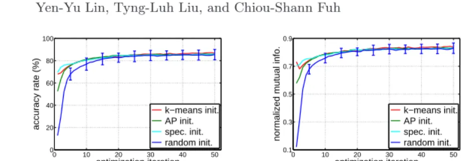
Fig. 2. With different initializations, the clustering accuracy (left) and normalized mutual information (right) of the proposed approach along the iterative optimization
Table 1 (top). In this setting, the proposed method outperforms k-means and affinity propagation, and is competitive with spectral clustering.
When multiple kernels are used simultaneously, we compare the proposed framework with cluster ensembles (CE) [18]. In particular, our implementation of cluster ensembles is to combine the five separately generated clustering results by one of the following three techniques: k-means, affinity propagation and spectral clustering. We report the results in Table 1 (bottom). First of all, our approach achieves significant improvements of 10.7% (= 85.7% − 75.0%) in ACC and 0.091 (= 0.833 − 0.742) in NMI over the best results obtained with a single kernel. It suggests that these kernels tend to complement one another, and our method can exploit this property to yield better clustering results. Furthermore, unlike that cluster ensembles relies on merging multiple clustering results in a global fashion, our approach performs cluster-dependent feature selection over multiple descriptors to recover the cluster structure. The quantitative results show that our method can make the most of multiple kernels, and improves the performances from 77.3% to 85.7% in ACC and from 0.758 to 0.833 in NMI.
Pertaining to the convergence issue, we evaluate our algorithm with 23 differ- ent initializations, including 20 random data partitionings and three meaningful clustering results by applying k-means, affinity propagation and spectral cluster- ing to kernel GB, respectively. The clustering performances through the iterative optimization procedure are plotted in Fig. 2. It can be observed that the pro- posed optimization algorithm is efficient and robust: It converges within a few iterations and yields similar performances with diverse initializations.
5.2 Face image grouping
Dataset The CMU PIE database [33] is used in our experiments of face image grouping. It comprises face images of 68 subjects. To evaluate our method for cluster-dependent feature selection, we divide the 68 people into four equal-size disjoint groups, each of which contains face images from 17 subjects reflecting a certain kind of variations. See Fig. 3 for an overview.
Specifically, for each subject in the first group, we consider only the images of the frontal pose (C27) taken in varying lighting conditions (those under the di-
(a) (b)
(c) (d)
Fig. 3.Four kinds of intraclass variations caused by (a) different lighting conditions, (b) in-plane rotations, (c) partial occlusions, and (d) out-of-plane rotations
(a) (b)
φ ψ′ ψ
Fig. 4.(a) Images obtained by applying the delighting algorithm [34] to the five images in Fig. 3a. (b) Each image is divided into 96 regions. The distance between the two images is obtained when circularly shifting causes ψ′to be the new starting radial axis
rectory “lights”). For subjects in the second and third groups, the images with near frontal poses (C05, C07, C09, C27, C29) under the directory “expression”
are used. While each image from the second group is rotated by a randomly sam- pled angle within [−45◦, 45◦], each from the third group is instead occluded by a non-face patch, whose area is about ten percent of the face region. Finally, for subjects in the fourth group, the images with out-of-plane rotations are selected under the directory “expression” and with the poses (C05, C11, C27, C29, C37). All images are cropped and resized to 51 × 51 pixels.
Descriptors, distances and kernels With the dataset, we adopt and design a set of visual features, and establish the following four kernels.
– DeLight. The data representation is obtained from the delighting algorithm [34], and the corresponding distance function is set as 1−cos θ, where θ is the angle between a pair of samples under the representation. Some delighting results are shown in Fig. 4a. It can be seen that variations caused by different lighting conditions are significantly alleviated under the representation.
– LBP. As is illustrated in Fig. 4b, we divide each image into 96 = 24 × 4 regions, and use a rotation-invariant local binary pattern (LBP) operator [35]
(with operator setting LBP8,1riu2) to detect 10 distinct binary patterns. Thus an image can be represented by a 960-dimensional vector, where each dimen- sion records the number of occurrences that a specific pattern is detected in the corresponding region. To achieve rotation invariant, the distance between two such vectors, say, xi and xj, is the minimal one among the 24 values computed from the distance function 1−sum(min(xi, xj))/sum(max(xi, xj)) by circularly shifting the starting radial axis for xj. Clearly, the base kernel is constructed to deal with variations resulting from rotations.
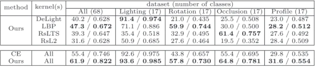
Table 2.The performances of cluster ensembles and our approach in different settings
dataset (number of classes) method kernel(s)
All (68) Lighting (17) Rotation (17) Occlusion (17) Profile (17) DeLight 40.2 / 0.628 91.4/ 0.974 21.0 / 0.435 25.5 / 0.508 23.0 / 0.487 LBP 47.3/ 0.672 71.1 / 0.886 59.9/ 0.744 30.0 / 0.500 28.2/ 0.512 Ours RsLTS 39.3 / 0.647 35.4 / 0.518 32.9 / 0.495 61.4/ 0.757 27.6 / 0.492
RsL2 31.6 / 0.628 50.9 / 0.685 27.6 / 0.464 19.5 / 0.352 28.4 / 0.509 CE All 55.4 / 0.746 92.6 / 0.975 43.8 / 0.657 55.4 / 0.695 29.8 / 0.535 Ours All 61.9/ 0.822 93.6/ 0.985 57.8/ 0.730 64.8/ 0.781 31.6/ 0.554
– RsL2. Each sample is represented by its pixel intensities in raster scan order.
Euclidean (L2) distance is used to correlate two images.
– RsLTS. The same as RsL2 except that the distance function is now based on the least trimmed squares (LTS) with 20% outliers allowed. The kernel is designed to take account of the partial occlusions in face images.
Quantitative results We report the performances of applying our approach to the four kernels one by one in the third column of Table 2 (top). Besides, we also record the performances with respect to each of the four groups in the last four columns of the same table. (Each group is named according to the type of its intraclass variation.) Note that each result in the last four columns is computed by considering only the data in the corresponding group. No additional clustering is performed. As expected, each of the four kernels generally yields good performances in dealing with a specific kind of intraclass variations. For example, the kernel DeLight achieves a satisfactory result for subjects in the Lighting group, while LBP and RsLTS yield acceptable outcomes in Rotation and Occlusion groups respectively. However, none of them is good enough for dealing with the whole dataset. Still the results reveal that if we could choose proper features for each subject, it would lead to substantial improvements.
To verify the point, we apply the proposed clustering technique to the four kernels simultaneously, and compare it with cluster ensembles, which is used to merge the four clustering results derived by implementing our approach with single kernel. In Table 2 (bottom), it shows that using multiple kernels in our approach can achieve remarkable improvements over the best result obtained from using a single kernel (i.e. LBP), and also significantly outperforms the foregoing setting for cluster ensembles.
Indeed performing clustering with this dataset is hard, due to the large sub- ject number and the extensive intraclass variations. We thus randomly generate one must-link and one cannot-link for each subject, and denote the setting of semisupervised clustering as 1M1C. Analogously, we also have 0M0C (i.e. unsuper- vised), 2M2C and 3M3C. Combining different amounts of pairwise constraints and different settings of kernel(s), the performances with respect to ACC and NMI of our approach are shown in Fig. 5. It is clear that by introducing only a few constraints, our approach can achieve considerable gains in performance.
0M0C 1M1C 2M2C 3M3C 30
40 50 60 70 80
accuracy rate (%)
Ours+All CE+All Ours+DeLight Ours+LBP Ours+RsLTS Ours+RsL2
0M0C 1M1C 2M2C 3M3C 0.6
0.7 0.8 0.9
normalized mutual info.
Ours+All CE+All Ours+DeLight Ours+LBP Ours+RsLTS Ours+RsL2
Fig. 5. The performances of cluster ensembles and our approach w.r.t. different amounts of must-links and cannot-links per subject and different settings of kernel(s)
6 Conclusion
We have presented an effective approach to clustering complex data that con- siders cluster-dependent feature selection and multiple feature representations.
Specifically, we incorporate the supervised training processes of cluster-specific classifiers into the unsupervised clustering procedure, cast them as a joint op- timization problem, and develop an efficient technique to accomplish it. The proposed method is comprehensively evaluated with two challenging vision ap- plications, coupled with a number of feature representations for the data. The promising experimental results further demonstrate its usefulness. In addition, our formulation provides a new way of extending the multiple kernel learning framework, which is typically used in tackling supervised-learning problems, to address unsupervised and semisupervised applications. This aspect of general- ization introduces a new frontier of applying multiple kernel learning to handling the ever-increasingly complex vision tasks.
Acknowledgments. We want to thank the anonymous reviewers for their valu- able comments. This work is supported in part by grant 97-2221-E-001-019-MY3.
References
1. Dueck, D., Frey, B.: Non-metric affinity propagation for unsupervised image cate- gorization. In: ICCV. (2007)
2. Tuzel, O., Porikli, F., Meer, P.: Kernel methods forweakly supervised mean shift clustering. In: ICCV. (2009)
3. Shi, J., Malik, J.: Normalized cuts and image segmentation. TPAMI (2000) 4. Comaniciu, D., Meer, P.: Mean shift: A robust approach toward feature space
analysis. TPAMI (2002)
5. Roth, V., Lange, T.: Feature selection in clustering problems. In: NIPS. (2003) 6. Ye, J., Zhao, Z., Wu, M.: Discriminative k-means for clustering. In: NIPS. (2007) 7. Lanckriet, G., Cristianini, N., Bartlett, P., Ghaoui, L., Jordan, M.: Learning the
kernel matrix with semidefinite programming. JMLR (2004)
8. Ng, A., Jordan, M., Weiss, Y.: On spectral clustering: Analysis and an algorithm.
In: NIPS. (2001)
9. Frey, B., Dueck, D.: Clustering by passing messages between data points. Science (2007)
10. Cheng, H., Hua, K., Vu, K.: Constrained locally weighted clustering. In: VLDB.
(2008)
11. Domeniconi, C., Al-Razgan, M.: Weighted cluster ensembles: Methods and analy- sis. TKDD (2009)
12. Berg, A., Malik, J.: Geometric blur for template matching. In: CVPR. (2001) 13. Lowe, D.: Distinctive image features from scale-invariant keypoints. IJCV (2004) 14. Lazebnik, S., Schmid, C., Ponce, J.: Beyond bags of features: Spatial pyramid
matching for recognizing natural scene categories. In: CVPR. (2006)
15. Bosch, A., Zisserman, A., Mu˜noz, X.: Representing shape with a spatial pyramid kernel. In: CIVR. (2007)
16. Xu, L., Neufeld, J., Larson, B., Schuurmans, D.: Maximum margin clustering. In:
NIPS. (2004)
17. Zhao, B., Wang, F., Zhang, C.: Efficient multiclass maximum margin clustering.
In: ICML. (2008)
18. Strehl, A., Ghosh, J.: Cluster ensembles – A knowledge reuse framework for com- bining multiple partitions. JMLR (2002)
19. Fred, A., Jain, A.: Combining multiple clusterings using evidence accumulation.
TPAMI (2005)
20. Xing, E., Ng, A., Jordan, M., Russell, S.: Distance metric learning with application to clustering with side-information. In: NIPS. (2002)
21. Mutch, J., Lowe, D.: Multiclass object recognition with sparse, localized features.
In: CVPR. (2006)
22. Zhang, H., Berg, A., Maire, M., Malik, J.: SVM-KNN: Discriminative nearest neighbor classification for visual category recognition. In: CVPR. (2006)
23. Lin, Y.-Y., Liu, T.-L., Fuh, C.-S.: Local ensemble kernel learning for object cate- gory recognition. In: CVPR. (2007)
24. Lin, Y.-Y., Tsai, J.-F., Liu, T.-L.: Efficient discriminative local learning for object recognition. In: ICCV. (2009)
25. Moghaddam, B., Shakhnarovich, G.: Boosted dyadic kernel discriminants. In:
NIPS. (2002)
26. Collins, M., Schapire, R., Singer, Y.: Logistic regression, AdaBoost and Bregman distances. ML (2002)
27. Friedman, J., Hastie, T., Tibshirani, R.: Additive logistic regression: A statistical view of boosting. Annals of Statistics (2000)
28. Wolsey, L.: Integer Programming. John Wiley & Sons (1998)
29. The MOSEK Optimization Software: (http://www.mosek.com/index.html) 30. Fei-Fei, L., Fergus, R., Perona, P.: Learning generative visual models from few
training examples: An incremental bayesian approach tested on 101 object cate- gories. In: CVPR Workshop on Generative-Model Based Vision. (2004)
31. Shechtman, E., Irani, M.: Matching local self-similarities across images and videos.
In: CVPR. (2007)
32. Cox, T., Cox, M.: Multidimentional Scaling. Chapman & Hall, London (1994) 33. Sim, T., Baker, S., Bsat, M.: The CMU pose, illumination, and expression database.
TPAMI (2005)
34. Gross, R., Brajovic, V.: An image preprocessing algorithm for illumination invari- ant face recognition. In: AVBPA. (2003)
35. Ojala, T., Pietik¨ainen, M., M¨aenp¨a¨a, T.: Multiresolution gray-scale and rotation invariant texture classification with local binary patterns. TPAMI (2002)