Travel Time Prediction for Urban Networks: the Comparisons of Simulation-based and Time-Series Models

Travel Time Prediction for Urban Networks: the

Comparisons of Simulation-based and Time-Series Models

Ta-Yin Hu

Department of Transportation and Communication Management Science.

National Cheng Kung University, No.1, Ta-Hsueh Road, Tainan 701, Taiwan, R.O.C.

TEL: 886-6-2757575-53224, FAX: 886-6-2753882, E-mail: [email protected] Wei-Ming Ho

Department of Transportation and Communication Management Science.

National Cheng Kung University, No.1, Ta-Hsueh Road, Tainan 701, Taiwan, R.O.C.

TEL: 886-6-2757575-5010, E-mail: [email protected]

ABSTRACT

Travel time prediction for urban networks is an important issue in Advanced Traveler Information Systems (ATIS) since drivers can make individual decisions, choose the shortest route, avoid congestions and improve network efficiency based on the predicted travel time information. In this research, two algorithms are proposed to estimate and predict travel time for urban networks, the simulation-based and time-series models. The simulation-based model, DynaTAIWAN, designed and developed for mixed traffic flows, is adopted to simulate the traffic flow patterns. The Autoregressive Integrated Moving Average (ARIMA) model, calibrated with vehicle detector (VD) data, is integrated with signal delay to predict travel time for arterial streets. In the numerical analysis, an arterial street in Kaohsiung city in Taiwan is conducted to illustrate these two models. The empirical and historical data are used to predict and analyze travel time, including: travel time data from survey and historical speed data from vehicle detector (VD).

INTRODUCTION

With the development of modern technologies in Intelligent Transportation Systems (ITS), the

route guidance with predicted travel time is an important issue, especially in Advanced

Traveler Information System (ATIS) [1]. Travel time is a key factor that can influence

drivers’ behavior, and can let travelers understand what kind of traffic situations they are

going to encounter while traveling [3]. Travel time is defined as the time required to travel

along a route between any two points within a traffic network [2][4].

With the development of new technologies, many instruments can be utilized to collect the traffic data, such as global positioning system (GPS), automated vehicle identification (AVI), and vehicle detector (VD). The travel time data can be directly/indirectly predicted through these technologies. Travel time can be estimated and predicted directly by using probe vehicles, license plate matching, electronic toll stations, and automatic vehicle identification (AVI) etc.; travel time can also be estimated and predicted indirectly by vehicle detectors (VD) [5].

Several approaches have been proposed for travel time estimation and prediction. Most of the statistical-based algorithms are based on the applications of regression, bayesian and time series models [6] [7] [8]. The models are based on historical/real time data to forecast the travel time. In general, the algorithms are easy to implement, but purely statistical-based algorithms may result in poor performance during abnormal traffic conditions [9]. The simulation-based method used traffic simulation software and can integrate other algorithms such as Kalman filter model and traffic flow theory model to simulate the traffic pattern [10].

Several empirical studies show that the extensive data needs to be collected for the model validation [3]. In summary, how to apply these algorithms under different traffic situations is still a critical issue and so far there is no conclusive evidence to demonstrate the best algorithm for travel time estimation and prediction.

This paper presents a simulation-based model and a time-series model for travel time estimation and prediction for urban networks. The simulation-based model, calibrated based on VD flow data, uses simulated vehicle trajectories to generate travel time information.

The ARIMA model, calibrated based on time-series data, is integrated with signal delay for travel time prediction. The simulation-based model is easy to be implemented with possible applications for normal and abnormal traffic conditions. The main advantage of ARIMA is its efficiency for short-term predictions.

The research framework for travel time prediction includes overall framework, simulation-based and time-series framework are described in next section. Numerical experiments and results are discussed in Sections 3 and 4, followed by brief summary.

RESEARCH FRAMEWORK

OVERALL FRAMEWORK

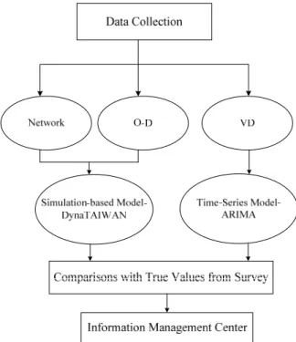
The overall framework of travel time estimation and prediction model is shown in Figure 1.

The collected input data sets for travel time model include network, O-D flows, and VD data.

The simulation-based model is calibrated based on the network and O-D data and the

time-series model is calibrated based on the historical data from VD. The true travel time values for validation are collected through probe vehicles.

Figure 1. The Overall Framework

SIMUALTION-BASED MODEL

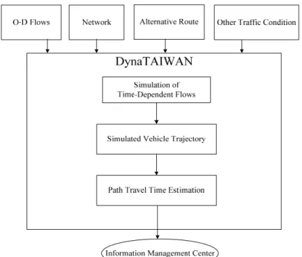
The framework of simulation-based travel time estimation and prediction is shown in Figure 2.

The input data sets for travel time model include O-D flows, network, alternative routes and

other traffic conditions. The time-dependent flow can be simulated through DynaTAIWAN,

and route travel time can be calculated based on the vehicle trajectory data.

Figure 2. The Conceptual Framework of Simulation-based Model

The travel time is directly calculated by averaging the travel time of vehicles start from origin node to destination node for each time interval, as described in the following equation:







k r s

s r k I

1 i

i s r k v

s r

k I

t T

, , , , ,

,

(1)

Where,

v s r

Tk_,,

is the vehicle-based average travel time from origin node r to destination node s during time interval k, and

i s r

tk_,,

is the average travel time of i vehicle from origin node r to destination node s during

time interval k.

The features of simulation-based model are summarized as follows:

(1) the algorithm is reliable since the vehicle trajectory is obtained through simulation.

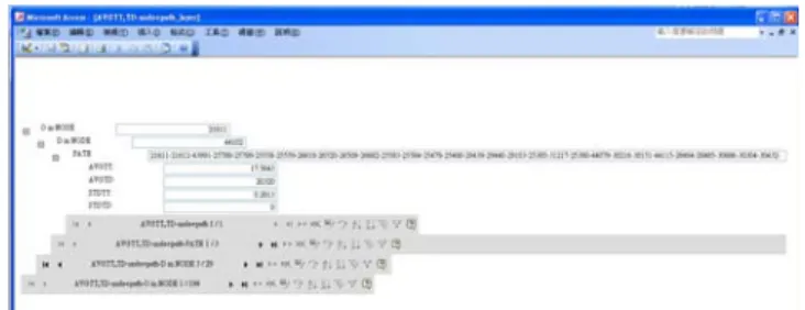
(2) The vehicle trajectory data is managed through relational data base management systems , such as Access, thus travel time information can be retrieved easily, as shown in Figure 3.

(3) The travel time, travel distance, and standard deviations from each origin to each can be obtained by identifying k the origin and destination numbers in database.

(4) The dynamic O-D estimation and prediction process needs to be incorporated with the

simulation model in order to obtain reliable simulation results.

Figure 3. The Simulation-based Database

TIME-SERIES MODEL

In time series analysis, an ARIMA model is a generalisation of an autoregressive moving average (ARMA) model. The common approaches for modeling univariate time series includes the autoregressive (AR) and the moving average (MA) models, and the ARIMA is a model after the combination of two models. The meaning of “I” in ARIMA model is

“Integrated”, and it means the time-series are differenced. ARIMA model can be applied to stationary time series, when the time series are non-stationary, they should be differenced.

These models are fitted to time series data either to better understand the data or to predict future points in the series.

The model is generally referred to as an ARIMA(p,d,q) model where p, d, and q are integers greater than or equal to zero and refer to the order of the autoregressive, integrated, and moving average parts of the model respectively.

The AR, MA, and ARMA model can be expressed as follows:

AR Model: Z

   

Z

 

Z

 ...  

Z

 a

(2)

MA Model: Z

   a

 

a

 

a

 ...  

a

(3)

ARMA Model: Z

   

Z

 

Z

 ...  

Z

 a

 

a

 

a

 ...  

a

(4) Where,

Z : time series



: constant a

 : the mean

p

1



 ...

 ... : parameters of the model



p: the order of the AR model

q: the order of the MA model

The determinations of p and q value in the ARIMA(p,d,q) model are based on the ACF and PACF index. They are briefly introduced below:



AR(p): ACF gradually tails off, and the PACF cuts off at time lag k when k > p.



MA(q): ACF cuts off at time lag k when k > q, and the PACF gradually tails off.



ARMA(p,q): Both ACF and PACF gradually tail off. The ACF exponentially tails off when the time lag is at q-p, and PACF tails off when the time lag is at p-q.

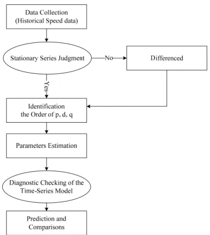
The procedure of time-series model is shown in Figure 4. The historical speed data are collected as the basic time series in the ARIMA model. If the historical time series are stationary, the order of p, d, q of the model can be identified initially, or the data needs to differenced before identification. The parameters of the ARIMA model can be estimated and diagnosed to check the parameters of the model and to determine the final time-series formulations. The final model can be applied to predict the objective time series and compared with the true value to verify the accuracy of the model.

Figure 4. The Procedure of Time-Series Model

MEASUREMENT CRITERIA

The MAPE indexes is applied to measure the performance of the models, the indexes is

calculated as in (5). The interpretation of MAPE index is shown in Table 1 [11].

) % (

) ( )

( 100

k x

k x k x M MAPE 1

M

1 k

 

  



(5)

Where,

M：the number of samples )

(k

x ： the real values )

(k

x ：the estimated values

Table 1. The Interpretation of MAPE Index [11]

MAPE (% ) Interpretation

<10 Highly accurate forecasting 10-20 Good forecasting 20-50 Reasonable forecasting

>50 Inaccurate forecasting

NUMERICAL EXPERIMENTS AND RESULTS

NETWORK CONFIGURATION

Numerical experiments are conducted for an arterial street in Kaohsiung city in Taiwan to illustrate these two models. The arterial street selected (the East bound and West bound) is located in the CBD with heavy traffic. The arterial street is shown in Figure 5. The East bound is from tag A to B and the node number is from 2616 to 5142. The West bound is from tag B to A and the node number is from 5142 to 2616. There are 8 intersections and 2 ramps in this arterial street.

Figure 5. The Arterial Street in the Experiments

DATA COLLECTION

The empirical travel time data is summarized in Table 2. The data is used in the comparison

process for the simulation-based model and the ARIMA model. The data is gathered from

7:30~8:00 AM in August 19, 2009.

Table 2. The Travel Time Data

1 2 3 Average Travel Time Stander Deviation East bound: 2616→5142 6.73 7.23 6.93 6.97 0.31

West bound: 5142→2616 6.33 6.43 6.9 6.56 0.15

（Unit: min）

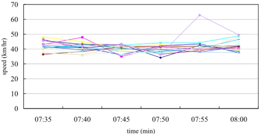
The historical speed data from 7:30~8:00 AM for 17 days is illustrated in Figure 6. The speed data is collected through VDs and the data is used in time series analysis.

Speed Temporal Distributions

0 10 20 30 40 50 60 70

07:35 07:40 07:45 07:50 07:55 08:00

time (min)

speed (km/hr)

Figure 6. The Temporal Distributions of Speed for 17 days

RESULTS ANALYSIS

Simulation-based Model

In order to observe the system performances under different demand levels, several loading factors are tested. The loading factor is defined as the ratio of the total number of vehicles generated in the network during the simulation period. The loading factors are tested from 0.5 to 0.9. The results show that the average travel time increases with respect to the loading factor. The results are shown in Table 3.

Table 3. The Predicted Travel Time with Simulation-based Model

Loading Factor 0.5 0.6 0.7 0.8 0.9 East Bound: 2616-5142 4.38 5.19 6.18 7.39 8.35 West Bound: 5142-2616 6.35 8.58 13.73 10.16 13.15

(Unit: min)

The empirical travel time data is compared with the predicted travel time by simulation-based model. The results are shown in Table 4. The results show that some MAPES values are less than 10%. For West bound prediction, the loading factor of 05 is more appropriate.

For East bound prediction, the loading factors of 0.7 and 0.8 are more appropriate. The

results indicate that time-dependent O-D demand data is very important in the simulation

model.

Table 4. The MAPE Values Comparisons with Simulation-based Model

West Bound: 5142-2616 0.67% 62.20% 783.67% 197.56% 662.01%

Time-series Model

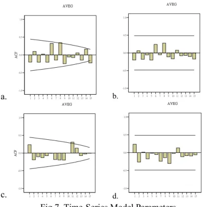
The signal cycle data are collected and used to calculate the expected delay for 8 intersections and 2 ramps, and the total expected delay is about 264.5 seconds. The time-series travel time prediction model is calibrated based on the 17 days’ historical speed data. The predicted travel time is basically calculated by the summation of the lengths for each links on the objective street divided by the predicted average speed. The ACF and PACF values for East bound and West bound streets are shown in Figure 7. The orders of the ARIMA model are listed in Table 5 and the models used are ARIMA(1,1,1) for East bound street and ARIMA(2,0,1) for West bound street.

a.

-1.0 -0.5 0.0 0.5 1.0

ACF

AVEG

b. ^{1 2 3 4 5 6 7 8 9} 10 11 12 13 14 15

落後數 -1.0

-0.5 0.0 0.5 1.0

AVEG

c.

-1.0 -0.5 0.0 0.5 1.0

ACF

AVEG

d. ^{1 2 3 4 5 6 7 8 9} 10 11 12 13 14 15

-1.0 -0.5 0.0 0.5 1.0

AVEG

Fig 7. Time-Series Model Parameters.

a. ACF for East bound street. b. PACF for West bound street.

c. ACF for East bound street. d. PACF for West bound street.

Table 5. The Order of the ARIMA Model

Parameters p d q (p,d,q)

East Bound: 2616-5142 1 1 1 (1,1,1)

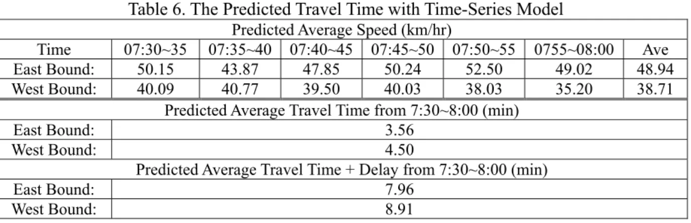
The predicted speed from 7:30~8:00 and average values on East bound street and West bound street are shown in Table 6. It shows that the time-series model can predict the travel time reasonably if the signal delay is included. The speed data from VDs does not able to reflect signal delay and possible reasons might be the location of installed VD.

Table 6. The Predicted Travel Time with Time-Series Model

Time 07:30~35 07:35~40 07:40~45 07:45~50 07:50~55 0755~08:00 Ave East Bound: 50.15 43.87 47.85 50.24 52.50 49.02 48.94 West Bound: 40.09 40.77 39.50 40.03 38.03 35.20 38.71

Predicted Average Travel Time from 7:30~8:00 (min)

East Bound: 3.56

West Bound: 4.50

Predicted Average Travel Time + Delay from 7:30~8:00 (min)

East Bound: 7.96

West Bound: 8.91

The best results from the simulation-based model and the ARIMA model are compared and the results are summarized in Table 7. Through these results, the simulation-based model shows possible potential for travel time prediction; however, the time-dependent O-D demand is still a crucial issue in applying the simulation-based model. For normal traffic conditions, the ARIMA model could also have reasonable results and the simulation-based model is applicable for abnormal traffic conditions.

Table 7. The Travel Time Comparisons

Model ARIMA DynaTAIWAN True Value

East Bound 7.96 7.39 6.97

West Bound 8.91 6.35 6.56

(Unit：min)

CONCLUDING COMMENTS

In this research, the simulation-based model based on DynaTAIWAN and the time-series with ARIMA model for travel time estimation and prediction are presented, and the empirical travel time data is collected for comparisons. The numerical results indicate the proposed simulation-based travel time prediction model and the ARIMA model provides reasonable travel time information.

Some important issues for time-series model include: (1) the accuracy of the model is

influenced by the outliers of the historical time-series; (2) the determinations of orders of p

and q may highly influence the performances. On the other hand, the network configuration

and time-dependent O-D demand data are very important in the simulation-based model, and these data sets can significantly influence the performances of travel time predictions.

ACKNOWLEDGEMENT

This paper is based on work supported by National Science Council, Taiwan, R.O.C. The authors would like to thank you for the help from students Chia-Hsin Yang and Yi Jie Wu.

Of course, the authors are solely responsible for the contents of this paper.

REFERENCES

(1) Chen M. and Chien I. J., “Dynamic Freeway Travel Time Prediction Using Probe Vehicle Data: Link-based vs. Path-base,” Transportation Research Record 1768, National Research Council, Washington, D. C., pp. 157–161, 2001.

(2) Ma X., Burghout W., and Koutsopoulos H., “Evaluation of Real-Time Travel Time Estimation Method and Disruption using Noisy Automatic Vehicle Identification Measurements,” Transportation Research Board 88th Annual Meeting, 2009.

(3) Tam M. L., and Lam W. H. K., “Short-term Travel Time Prediction for Congested Urban Road Networks,” Transportataion Research Board 89th Annual Meeting, 2009.

(4) Ben-Akiva, M., De Palma, A., and Kaysi, I., “Dynamic network models and driver information systems,” Transportation Research 25A (5), pp. 251–266, 1991.

(5) Vanajakshi L., Subramanian S. C., and Sivanandan R., “Short term prediction of travel time for Indian traffic conditions using buses as probe vehicles,” Transportation Research Board 87th Annual Meeting, 2008.

(6) Lam S. H. and Toan T. D., “Short-Team Travel Time Prediction Using Support Vector Regression,” Transportation Research Board 87th Annual Meeting, 2008.

(7) Hinsbergen V. and Lint V., “Bayesian Combination of Travel Time Prediction Models,”

Transportation Research Board 87th Annual Meeting, 2008.

(8) Guin A., “Travel Time Prediction Using a Seasonal Autoregressive Integrated Moving Average Time Series Model,” Proceedings of the 9th IEEE International Conference on Intelligent Transportation system, pp. 493–498, 2006.

(9) Ishaak, S. and Al-Deek, H., “Statistical Evaluation of I-4 Prediction System,”

Transportation Research Board 83th Annual Meeting, 2003.

(10) Liu Y., Lin P. W., Lai X., Chang G.L., and Marquess A., “Developments and Applications of a Simulation-Based Online Travel Time Prediction System,” Transportation Research Record 1959, National Research Council, Washington, D. C., pp. 92–104, 2006.

(11) Lewis, C. D. (1982), Industrial and Business Forecasting Methods, London:

Butterworths.