國 立 交 通 大 學
電信工程學系
碩 士 論 文
跨環的彈性分封環網路之
智慧型全域公平控制器
Intelligent Global Fairness Controller in
Bridged Resilient Packet Ring Networks
研 究 生:吳英奇
指導教授:張仲儒 博士
跨環的彈性分封環網路之智慧型全域公平控制器
Intelligent Global Fairness Controller
in Bridged Resilient Packet Ring Networks
研 究 生:吳英奇 Student:Ying-Chi Wu
指導教授:張仲儒 博士 Advisor:Dr. Chung-Ju Chang
國立交通大學
電信工程學系
碩士論文
A Thesis
Submitted to Department of Communication Engineering
College of Electrical and Computer Engineering
National Chiao Tung University
in Partial Fulfillment of the Requirements
for the Degree of Master of Science
in
Communication Engineering
July 2008
Hsinchu, Taiwan
跨環的彈性分封環網路之智慧型全域公平控制器
研究生:吳英奇 指導教授:張仲儒 博士
國立交通大學電信工程學系碩士班
Mandarin Abstract
摘 要 IEEE 在標準 802.17 中提出了一個適用於下一代都會區域網路(Metropolitan Area Network)的彈性分封環(Resilient Packet Ring)架構。基於頻寬的需求,以及 為了服務更廣大的區域,多個彈性分封環可以橋接在一起,形成一個跨環的彈性 分封環網路。先前的研究著重在於整個跨環的彈性分封環網路的拓墣發現,以減 少泛流式(flooding)廣播的方式來傳送跨環的資料。另外也有專注於確保跨環的資 料能夠達到全域公平性的研究,但是他們並不能完全保證不會有緩衝區溢位的情 形發生。目前已經有許多關於單一個彈性分封環之本地的公平演算法被提出,但 是本地的公平演算法並不適用在跨環的資料所需要達到的全域公平性。因此,我 們根據一個稱之為Ring Ingress Aggregated with Spatial Reuse (RIAS)的本地性公 平定義,發展出一套全域性的公平準則,並且提出一個智慧型全域公平控制器。 這個智慧型全域公平控制器能提供全域公平、維持本地性公平,而且完全對緩衝 區溢位的問題免疫。另外我們也提出一個權重路徑選擇器,藉著有效率的判斷, 來選擇沒有被使用的路徑來傳送資料,以提升系統的頻寬使用率。在模擬結果中 可以發現,針對不同的拓墣網路環境以及不同的資料需求模式,智慧型全域公平 控制器都有著良好的表現。Intelligent Global Fairness Controller
in Bridged Resilient Packet Ring Networks
Student:
Ying-Chi
Wu Advisor:
Chung-Ju
Chang
Department of Communication Engineering National Chiao Tung University, Taiwan
English Abstract
Abstract
Resilient Packet Ring (RPR) is designed for the next generation Metropolitan Area Network (MAN), also known as the IEEE 802.17 standard. Multiple RPRs can be connected together to from a bridged RPR network (BRPR) to support the wide area and the growing demands of bandwidth. Previous researches have focused on topology discovery without flooding inter-ring traffic, whose source and destination nodes are on different rings; also, assurance of global fairness for inter-ring traffic but not always immune to buffer overflow. Many local fairness algorithms have been proposed, but they are unable to ensure fairness for inter-ring traffic. So, we develop the global fairness criteria inherited from RIAS local fairness reference model. Then we propose an intelligent global fairness controller (IGFC) to provide global fairness for inter-ring traffic, maintain local fairness for intra-ring traffic, and guarantee the immunity against buffer overflow. A simple weighted ringlet selector (WRS) is also proposed to promote bandwidth utilization by employing the unused ringlet. We justify that IGFC achieve better performance under various topology and traffic patterns.
誌謝
Acknowledgements
碩士的訓練在本篇論文的完成也同時告一段落。兩年中所學到的寶貴知識與做 事的方法、態度,使我獲益匪淺,也改進了我的缺點。回顧這兩年,首先要感謝恩 師張仲儒教授在論文上的悉心指導,還有在生涯規劃上的諄諄教誨,更不時耳提面 命,告訴我們行事工作應有的謹慎積極的態度,培養我們未來在職場上的競爭力。 其次要感謝文祥學長總是不厭其煩的與我討論論文問題,點破我的盲點。謝謝立峰、 志明、振宇、耀興、芳慶、詠翰學長們適時的給我建議,使我不會一直陷入無窮的 迴圈。特別感謝維謙,經常三更半夜跟我ㄧ起寫程式,即使是在漫步回車棚、宿舍 的時候,也都在討論論文的細節。兩年的研究生活轉瞬即逝,其中的歡笑與淚水讓 我有著無限的感動與回憶。感謝建興、正昕、世宏、佳泓、佳璇、建安、尚樺等學 長姐,一起同甘共苦的邱胤、宗利、巧瑩、浩翔,以及盈予、和儁、欣毅及志遠等 學弟妹,還有熱情的助理玉棋,我永遠記得大家一起出遊、打球的快樂日子,也間 接磨練我的籃球技巧更上層樓。很開心加入寬頻網路實驗室這個大家庭,也祝福實 驗室的大家學業順利,事業有成! 最後,謹以此篇論文獻給我最摯愛的父母、妹妹,和家人,即便家裡遇到種種 難關,還是全心全力的支持我,使我無後顧之憂,謝謝您們!願您們與我分享這份 喜悅,並且與我一起迎接美好的未來。 英奇 謹誌 民國九十七年七月Contents
Mandarin Abstract ... i English Abstract... ii Acknowledgements ... iii Contents... iv List of Figures ... viList of Tables ... vii
Chapter 1 Introduction ...1
1.1 RPR Background ... 2
1.2 Local Fairness... 3
1.3 Issues with Bridged Resilient Packet Ring... 5
1.4 Previous Research on BRPR ... 6
1.5 Proposed Intelligent Global Fairness Controller ... 7
Chapter 2 System Model ...9
2.1 Architecture of Bridged RPR Network... 9
2.2 Architecture of Bridge Node... 10
2.3 Spatially Aware Sublayer (SAS)... 12
2.3.1 Current Research about Bridge Routing... 12
2.3.2 Weighted Ringlet Selector (WRS)... 13
Chapter 3 Intelligent Global Fairness Controller...15
3.1 Architecture of IGFC... 15
3.2 Local Fairness at Bridge ... 17
3.3 Global Fairness Criteria... 18
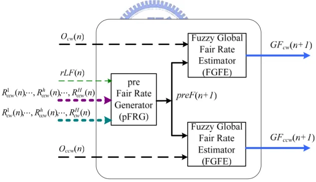
3.4 Global Fair Rates Generator... 19
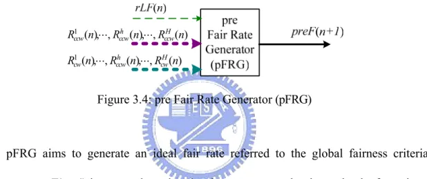
3.4.1 pre Fair Rate Generator (pFRG)... 20
3.4.2 Fuzzy Global Fair Rate Estimator (FGFE)... 22
3.5 Traffic Scheduling ... 27
3.6 Transiving Global Fairness Packets ... 28
Chapter 4 Simulation Results and Discussions...29
4.1 Simulation Environment... 29
4.2 Small Topology Scenario ... 31
4.3 Large Topology Scenario ... 34
4.4 Dynamic Traffic Scenario ... 38
4.5 Unbalanced Traffic Scenario... 41
Chapter 5 Conclusions ...45
Bibliography...47
List of Figures
Figure 1.1: Illustration of RIAS fairness ... 3
Figure 1.2: Illustration of spatial reuse………3
Figure 2.1: A simple RPR bridged network ... 9
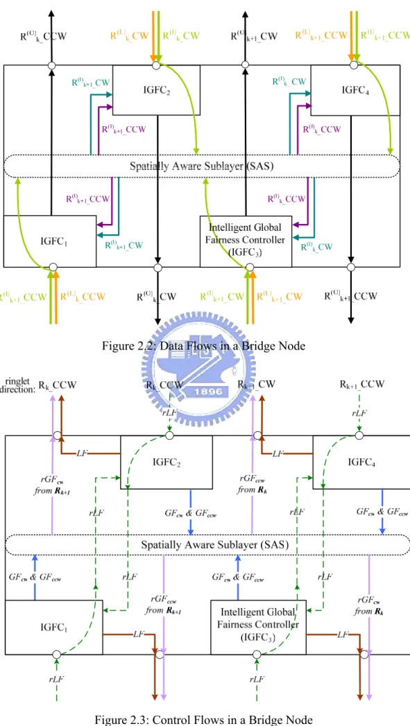
Figure 2.2: Data Flows in a Bridge Node... 11
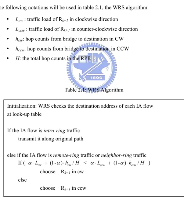
Figure 2.3: Control Flows in a Bridge Node ... 11
Figure 3.1: Intelligent Global Fairness Controller... 16
Figure 3.2: Local Fairness Controller of a Local Station ... 17
Figure 3.3: Global Fair Rates Generator (GFRG)... 19
Figure 3.4: pre Fair Rate Generator (pFRG) ... 20
Figure 3.5: Fuzzy Global Fair Rate Estimator (FGFE) for CW ringlet ... 22
Figure 3.6: The membership function of the term sets (a) T(Ocw(n)), (b) T(preF(n+1)), and (c) T(GFcw(n+1))... 25
Figure 4.1: Small Topology Scenario. (a) Scenario Setup (b) Average Access Delay at Bridge, (c) IGFC, and (d) RGFC... 32
Figure 4.2: Large Topology Scenario. (a) Scenario setup, (b) Throughput by IGFC, (c) Throughput by RGFC, (d) Dropping Probability at Bridge, (e) Transmission Rate of each source node by IGFC, and (f) Transmission Rate of each source node by RGFC... 36
Figure 4.3: Simple Rate Changing Scenario. (a) Scenario Setup, (b) IGFC, (c) RGFC, and (d) IGFC with WRS ... 40
Figure 4.4: Unbalanced Traffic Scenario. (a) Scenario setup, (b) IGFC, (c) RGFC, and (d) Dropping Probability at Bridge... 43
List of Tables
Table 2.1: WRS Algorithm ... 14
Table 3.1: The rule base of fuzzy global fair rate estimator ... 26
Table 4.1: System Parameters... 29
Chapter 1
Introduction
Resilient packet ring (RPR), a new packet-switching high-speed backbone technology for metropolitan and wide area networks, is proposed in IEEE 802.17 [1]. A synchronous optical network (SONET) ring and a Gigabit Ethernet (GigE) are the two well-known predecessors that have dominated the metropolitan area network architecture over the past ten years. SONET, which has dual ringlets and is implemented by circuit switching, is guaranteed to support fast link failure recovery and minimum bandwidth and delay. However, the other ringlet is reserved for protection and is unused during normal operation. GigE assures ease of manageability and low cost, simple traffic prioritization rules and full statistical multiplexing. Nevertheless, GigE suffers from unfairness because it implements proportional fairness algorithm and nodes will obtain different throughputs depending on their spatial location on the network. RPR can not only be compatible with current network architectures, SONET and GigE, but also mitigate their underutilization and unfairness problems. Besides, RPR can be expanded by bridging multiple RPRs to from a bridged RPR network (BRPR) when necessary. In the bridged RPR, two critical issues are accompanied. First, congestion is easily happened at bridge for inter-ring traffic whose source and destination nodes are on different rings. Second, there is no mechanism
which can guarantee global fairness for inter-ring traffic while obeying local fairness. Consequently, it is possible to have packet loss at bridge and unfair bandwidth allocation for inter-ring traffic. In this thesis, we will propose an intelligent global fairness
controller to efficiently administrate the bandwidth allocation and solve the buffer
overflow problem in the bridge.
1.1 RPR Background
RPR consists of two optical rotating ringlets which provide bidirectional transmission and link failure recovery by using the other ringlet instead of discarding packets when several links failed. This feature is so called “resilience”. The key performance objectives of RPR are to achieve high bandwidth utilization, fair share bandwidth for each node and optimum spatial reuse. Comparing with IEEE 802.5 which
uses source-stripping that only one node can transmit packets at the same time while getting the token, RPR removes packets from the ring at the destination node – destination stripping – in order that unused segments of the ring can be used at the same time for different flows [2, 3]. By this feature, RPR can achieve high bandwidth utilization.
How do we allocate each flow’s rate fairly? How do we avoid any node’s starvation or congestion when multiple flows are through a node in transit? Yuan, Gambiroza, and Knightly proposed a ring ingress aggregated with spatial reuse (RIAS). This is a fairness reference model [4] and has been included in the IEEE 802.17 standard’s targeted performance objective. First, RIAS fairness defines a basic unit for fairness at a link as an ingress-aggregated (IA) traffic flow—the aggregate of all sub-flows originating from a given ingress node. Then, the RIAS fairness guarantees that each IA flow on the most congested link equally share the available bandwidth. Finally, it ensures an optimum
spatial reuse so that the remaining bandwidth can be reclaimed for some unsatisfied flows after fair share on each IA flow.
RPR RIAS fairness and spatial reuse features can be simply illustrated by two parking lot scenarios in Figures 1.1 and 1.2, respectively. Each flow is assumed to be with infinite demand. In Figure 1.1, each flow should achieve the max target, 0.25 of the link bandwidth, to ensure equal share for each IA flow. Figure 1.2 is an extended case of Figure 1.1 with added flow (1, 3) and flow (4, 6). IA(4) is aggregated from flow (4, 5) and flow (4,6). On the most congested link 4, each IA flow is equally shared; that is, IA(1), IA(2), IA(3) and IA(4) get 0.25, while flow (4, 5) and flow (4, 6) get half of IA(4) traffic. What is more, to fully archive spatial reuse, the remaining bandwidth at link 1 and link 2 will be used as more as possible; thus, flow (1, 3) reclaims 0.5 capacity.
Figure 1.1: Illustration of RIAS fairness Figure 1.2: Illustration of spatial reuse
1.2 Local Fairness
IEEE 802.17 specified aggressive mode [2, 5] (AM) and conservative mode [2, 6] (CM) operations, which are approaching RIAS fair, to aim at fairness of intra-ring traffic. In every agingInterval (a computation period 100μs), each node conveys a local fairness control packet containing a new local fair rate (LF) to upstream nodes to adjust their add
rate. If the node and downstream nodes are not congested, the transmitting LF equals FULL_RATE which is link capacity per agingInterval. FULL_RATE means upstream nodes are able to ramp up their add rates. Otherwise, the node selects a smaller one to advertise between the locally computed LF and the received LF from the downstream node. In the AM mode, a node generates local fair rate (LF) in terms of add rate only if the STQ occupancy exceeds the low threshold. In CM mode, LF is the unreserved bandwidth divided by the number of active nodes where an upstream node is considered as active if received traffic was transmitted by upstream nodes. However, the feature of adjusting rate in both modes incurs rate oscillation, particularly in unbalanced traffic scenario (very different traffic demand in every flow). The violent oscillation at the transient state is a barrier to achieve an optimum spatial reuse, a fast convergence time and a high bandwidth utilization.
Several local fairness algorithms were proposed [7, 8, 9, 10] to solve the encountered problem in AM and CM. E. Knightly et al. proposed a distributed virtual time scheduling
in ring (DVSR) algorithm [7] with moderate oscillation at the transient state. DVSR used
a generalized processor sharing (GPS) system to compute the virtual time of each IA flow so that the traffic demand of upstream nodes and congested state at downstream node can be measured to estimate LF. The estimated LF and the throughput of each node is RIAS fairness. However, the drawback of DVSR has high computational complexity, which is with O(NlogN). Hence, Ansari and Alharbi proposed a distributed bandwidth allocation (DBA) [8] with the advantage of constant complexity, O(1), and a simple scheduling algorithm (SSA) [9], referred to DBA’s method, in addition to using virtual destination queues (VDQ) to avoid head of line blocking. DBA declares arrival rate and add rate divided by previous local fair rate as effective number of flows. In terms of effective
number of flows and the remaining available bandwidth, DBA computes the present local fair rate by means of Newton’s method. It is not unique that a novel fairness mechanism in [10] is also based on the effective number of flows.
1.3 Issues with Bridged Resilient Packet Ring
Multiple RPR rings can be connected together to form a larger network to satisfy metropolitan areas and the dramatically increasing bandwidth demand. As shown in Figure 2.1, this is a bridged-RPR network (BRPR) where the bridge node can connect two or more single rings. We will use the term ringlet to refer to one of the dual rings in RPR and the term ring to refer to a single RPR in BRPR.
In order to maintain the same efficiency and performance as the single RPR ring, the bridge node plays an important role in BRPR. On the one hand, according to the destination address recording on inter-ring packets, the bridge must choose a better path from one of two ringlets such that packets can reach their destination efficiently. It is called ringlet selection and is implemented at spatially aware sublayer (SAS) of IEEE 802.17b [11], an essential optional sublayer of bridge MAC layer, on which the IEEE 802.17 Working Group is still working. SAS not only resolves which ringlet packets should be forwarded to but also provides spatial reuse in the use of directed transmission through the destination address carried on inter-ring packets. Without SAS, BRPR seems like a broadcast medium for inter-ring packets and they are flooded onto the neighbor ring.
On the other hand, the bridge has to coordinate the transmitting rate of inter-ring and intra-ring traffic if congestion at bridge occurs. As long as intra-ring and inter-ring traffic are bounded for the same ringlet, it is highly probable that traffic aggregating at bridge is
much greater than the available bandwidth of the output link. Thus, the amount of the buffer at bridge would grow, which will induces buffer overflow. Besides, the other dilemma is called global fairness problem for bridged RPR network that certain nodes may monopolize most of the available bandwidth and then some nodes are in starvation.
1.4 Previous Research on BRPR
Setthawong and Tanterdtid proposed a RIAS based global fairness controller (RGFC) to ensure inter-ring traffic in the achievement of global fairness, [12]. The RGFC consists of a local ringlet buffer and an ingress buffer to accommodate intra-ring traffic and inter-ring traffic, respectively. The RGFC publishes a global fair rate, denoted by GF, into two ringlets every agingInterval. When the unfairness indicator is invoked, RGFC computes a GF. Otherwise, GF is always set to a special value, FULL_RATE. The unfairness indicator is composed of two conditions. First, the current received local fair rate at the present agingInterval is smaller than the previous one. Second, the STQ length of ingress buffer is larger than the threshold of STQ size.
As for the threshold of buffer length, it is to prevent buffer overflow as well. However, it is invalid while many nodes are in a BRPR network. This is because the influence of propagation delay makes the arrival rate of each inter-ring traffic flow very different at the transient state. Thus, the calculated GF is probably over adjusted as it follows global fairness criteria and depends on each flow’s arrival rate. Next, the total arrival traffic to bridge for next agingInterval is larger than the available bandwidth such that the buffer fills up and buffer overflow occurs. This easily loses fairness and delay the convergence time while the bridge drops packets at tail and the traffic of random source nodes is blocked outside. So they brought up a dropped algorithm to guarantee global
fairness and somehow ensure buffer overflow prevention. If the arrival rate of the source node is larger than GF, the extra packets are discarded, even though the buffer is not yet full. Obviously, it is unreasonable that dropping packets is still usually happened instead of buffer overflow.
Although only an ingress buffer queues inter-ring traffic from clockwise (CW) and counter-clockwise (CCW) direction, it costs more expense to approach every inter-ring flow to global fairness criteria due to first-in-first-out discipline. These will induce the performance degradation on the convergence time, oscillations, and buffer overflow.
1.5 Proposed Intelligent Global Fairness Controller
We are supposed to focus on how to prevent packets from being dropped at the bridge; how to maintain local fairness while doing global fairness at the same time; finally how to deal with unbalanced traffic in global fairness algorithm since it have significant effects on local fairness algorithm, AM and CM. We develop an intelligent global fairness controller (IGFC). It seems like a local station which is used to keep and forward transiting traffic, maintain local fairness, but also support global fairness.
Differently, there are two buffers to store inter-ring traffic from two different ringlet directions. Also there is a global fair rates generator (GFRG) to generate two distinct global fair rates, GFcw and GFccw, for upstream nodes whose inter-ring traffic is
transmitting in CW and CCW direction, respectively. The generator is divided into two stages. The first stage is a pre fair rate generator (pFRG) to compute an accurate fair rate according to max min mechanism and global fairness criteria. The second stage is a fuzzy global fair rate estimator (FGFE). As implied by the name, we adopt fuzzy control to estimate global fair rate intelligently according to the occupancy of the buffer and the pre
fair rate by the previous stage. Moreover, the dynamic weighted round robin scheduling is used to manipulate inter-ring traffic out of buffers precisely subject to global fairness
criteria. Therefore, a fast convergence time without buffer overflow can be expected.
The remainder of this thesis is organized as follows. Chapter 2 depicts the data-flow and the fairness-flow diagrams at a bridge to more understand the bridge operation. At the end of Chapter 2, we propose a weighted ringlet selector (WRS) for each data flow to choose a better ringlet to go across the bridge. In Chapter 3, the architecture of intelligent global fairness controller is introduced. We define the global fairness criteria and describe the design principle of the IGFC in detail. Then Chapter 4 presents performance evaluation for different configurations and comparisons among RGFC. Finally, Chapter 5 concludes this thesis.
Chapter 2
System Model
2.1 Architecture of Bridged RPR Network
Consider a simple bridged RPR network, where a bridge node Bk connects Rk RPR
ring and Rk+1 RPR ring, as shown in Figure 2.1. A ring consists of two unidirectional and
counter-rotating ringlets. Nodes can transmit packets in clockwise direction (CW) by using the outer-ringlet–ringlet 0, and also forward packets in counter-clockwise direction (CCW) by using the inner- ringlet–ringlet 1.
2.2 Architecture of Bridge Node
Bridge is a medium for two or more rings (two rings in this thesis), yet doesn’t generate traffic itself. A rule needs to be mentioned at Bk that traffic from Rk in CW can
not go to the same ring in CCW, but may leave for Rk+1 by either direction. Figure 2.2 is a
data flows diagram and Figure 2.3 is a control flows diagram in Bk. As shown in Figure
2.2, conceptually, there are four proposed intelligent global fairness controllers (IGFC) which are input and output interfaces to manage inter-ring and intra-ring traffic. To describe these two diagrams, we take a scenario for example that inter-ring traffic from Rk
in CW and CCW is going to Rk+1 in CCW through IGFC4.
R(L)
k_CW and R(I)k_CCW are traffic originating from Rk in CW. The former is the
local traffic still going to Rk in CW; however the latter is the inter-ring traffic bounding for
Rk+1 in CCW. IGFC1 recognizes R(I)k_CW as inter-ring traffic and delivers it directly to
SAS. Similarly, R(I)
k_CCW is also forwarded to SAS across IGFC2. Inter-ring traffic
enters SAS and the weighted ringlet selector (WRS) in chapter 2.4, a part of SAS, will select an optimal resolution of each inter-ring IA (IIA) flow from corresponding IGFCs. IGFC4 integrates and transmits local traffic: R(L)k+1_CCW and inter-ring traffic: R(I)k_CW
or R(I)
k_CCW, to output R(O)k+1_CCW. Therefore, each interface of Bk occurs congestion
easier than local stations because three kinds of traffic are bound for the same output link. In a RPR ring, nodes send and receive a local fairness control packet during every agingInterval and a fairness packet is transmitted via the opposing ringlet direction. Likewise in a BRPR network, IGFCs not only periodically send and receive a local fairness packet; but also periodically deliver global fairness packets. IGFC4 receives the
local fair rate (rLF) from the downstream node next to bridge via the opposing ringlet bypassing IGFC3.
Figure 2.2: Data Flows in a Bridge Node
We reset the received local fair rate to be the maximum of the output rate of inter-ring traffic modified from PerAgingInterval state machine of IEEE 802.17. Also,
rLF can be used to generate global fair rate (GF). IGFC4 produces two distinct GFs. GFcw
is used to inform nodes on Rk which transmit inter-ring traffic in CW; and so is GFccw.
Nonetheless, it is possible that IGFC3 generates GFcw because some inter-ring traffic also
comes from Rk in CW. Thus, SAS will pick the smaller GFcw and deliver it to the
corresponding ringlet. In addition to generating GFs, IGFC4 has to produce LF. Despite a
dissimilar architecture of IGFC from local fairness controller of a local station, we imitate AM local fairness algorithm to generate LF. We will depict the architecture of IGFC and explain the design principle in Chapter 3.
2.3 Spatially Aware Sublayer (SAS)
2.3.1 Current Research about Bridge Routing
SAS is the sublayer of the bridge MAC layer and its functionality is to provide spatial reuse. Bridge MAC inherits part of transparent bridges, as defined in IEEE Std. 802.1D, [13], also mentioned in Annex F of Std. 802.17. This standard is applied to a shared broadcast medium network, like Ethernet, where all stations can listen to all packets. Two bridging algorithms have been proposed: basic bridging algorithm was in 802.17b draft and F. Davik et al. proposed enhanced bridging algorithm [14]. Basic bridging uses flooding while still maintaining the spatial reuse property for local traffic. Consequently, inter-ring packets are flooded on all the rings but not on the shortest path; that is to say, RPR bridged network works like a shared medium network for inter-ring traffic. It declines the bandwidth efficiency and does not achieve spatial reuse for
inter-ring traffic.
Enhanced bridging algorithm is a better bridging strategy because it doubles the bandwidth efficiency and improves better latency in contrast with basic bridging. This strategy makes every station be equipped with a spatial reuse control sublayer table (SRCS). SRCS tables records all inter-ring stations (global stations) address and their corresponding local bridge. However, enhanced bridging needs flooding in the beginning until SRCS tables are completed. In spite of the initial learning and constructing process, the enhanced bridging algorithm provides spatial reuse also for inter-ring traffic.
2.3.2 Weighted Ringlet Selector (WRS)
Our proposed weighted ringlet selector is part of SAS and decides a ringlet which inter-ring traffic flows are forwarded on. Inter-ring traffic includes neighbor-ring or remote-ring traffic. It has much effect on bandwidth utilization and system performance to avoid most inter-ring flows going to the same ringlet. We consider average traffic load, total nodes in a ring and hop counts from bridge to destination as influential factors to make decisions. Buffer occupancy is not concerned since IGFC is used to resolve buffer overflow. One thing needs to be mentioned that WRS does not decide the path packet by packet because the destination node will receive traffic out of order and it is not suitable for optical transmission. WRS chooses a path by an inter-ring IA flow. Throughout the WRS algorithm, we consider inter-ring IA flows are from Rk to Rk+1 through Bk. and we
assume the bridge has learned the topology of the BRPR.
Criterion: The weighted ringlet decision expression is a cost function denoted by
C, which is defined as
where α is a weighted parameter between 1 and 0, L is the average traffic load per agingInterval, h is hop counts from bridge to destination node, and H is the total hop counts in the RPR ring. When α is 0, choose path only based on hop counts; when α is 1, choose path only based on traffic load. We always choose the lighter path according to Eq. (2.1).
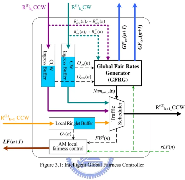
2.3.3 WRS Algorithm
The following notations will be used in table 2.1, the WRS algorithm. y Lcw : traffic load of Rk+1 in clockwise direction
y Lccw : traffic load of Rk+1 in counter-clockwise direction
y hcw: hop counts from bridge to destination in CW
y hccw: hop counts from bridge to destination in CCW
y H: the total hop counts in the RPR
Table 2.1: WRS Algorithm
Initialization: WRS checks the destination address of each IA flow at look-up table
If the IA flow is intra-ring traffic transmit it along original path
else if the IA flow is remote-ring traffic or neighbor-ring traffic If ( α⋅Lcw + (1- )α ⋅hcw/H < α⋅Lccw + (1- )α ⋅hccw/H ) choose Rk+1 in cw
else
Chapter 3
Intelligent Global Fairness Controller
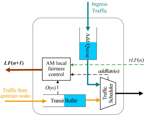
3.1 Architecture of IGFC
Figure 3.1 is the architecture of an intelligent global fairness controller. The main purposes of IGFC are to maintain local and global fairness and to prevent buffer overflow. We will still focus on IGFC4 based on our scenario in Chapter 2.2. There are a CW ingress
buffer, a CCW ingress buffer and a local ringlet buffer to temporarily store inter-ring traffic from Rk in CW, CCW and intra-ring traffic from Rk+1 in CCW, respectively.
Referred to the MAC transit dual queue design of a local station in standard, each buffer has two queues: primary transit queue (PTQ) and secondary transit queue (STQ); both are FIFO queues. The RPR MAC separates data from Class A, B and C. Class A provides a guaranteed bandwidth with low end-to-end delay and has priority over Class B and Class C. Class A traffic is placed into PTQ. Class B is near real time traffic with bounded delay. It has precedence over Class C traffic. Class C traffic provides best-effort traffic service with no guaranteed bandwidth and no bounds on end-to-end delay. Both Class B and Class C traffic are put into STQ. Only Class C traffic is subjected to the fairness algorithm and called fairness eligible traffic.
Global Fair Rates Generator (GFRG) R(I) k_CW R(I)k_CCW R(L)k+1_CCW rLF(n) R(O) k+1_CCW LF(n+1) Ocw(n) Occw(n) OL(n) Numcw/ccw(n) 1 ( ), ( )H cw cw R n ⋅⋅⋅R n 1 ( ), ( )H ccw ccw R n ⋅⋅⋅R n FWI(n) Local Ringlet Buffer
Figure 3.1: Intelligent Global Fairness Controller
rLF is the available inter-ring traffic bandwidth. Without GF, some nodes may
monopolize the available inter-ring traffic bandwidth and other nodes may get an unfair share. Rate monitor counts the arrival rate of each node’s fairness eligible traffic individually from arriving inter-ring traffic: h
cw
R or h ccw
R , whose superscript means the node
is “h” hop-counts to bridge and subscript means where the traffic comes from. Ocw and
Occw are the STQ occupancy of each ingress buffer. Upon above parameters, global fair
rates generator (GFRG) is able to publish GFcw(n+1) and GFccw(n+1) to upstream nodes
for next agingInterval. As for Numcw(n) and Numccw(n), they are intermediate products
from GFRG and used to control the output rate of STQ of CW/CCW ingress buffer. Before generating GF, the global fairness criteria will be introduced in Chapter 3.3. Next, GFRG and traffic scheduling will be described in Chapter 3.4 and 3.7, respectively.
3.2 Local Fairness at Bridge
In order to implement local fairness at bridge, IGFC can be somehow regarded as a local station as shown in Figure 3.2. When STQ occupancy of transit buffer (O(n)) is larger than the low threshold, AM detects the station congested and sets addRate(n), which is forward rate of fairness eligible traffic of add queue out of the station, as the locally computed fair rate.
Traffi c Scheduler A dd Q ue ue
Figure 3.2: Local Fairness Controller of a Local Station
Therefore, we can consider CW/CCW ingress buffers as add queues and local ringlet buffer as transit buffer. If OL(n) exceeds STQ low threshold, locally computed fair rate is
counting the summation of forward rate of fairness eligible inter-ring traffic at CW and CCW ringlet buffers, denoted by FWI(n). rLF is used to compute allowedRateCongested at which inter-ring traffic transiting the bridge can be added to the ringlet. In the presence of downstream congestion, allowedRateCongested is the recently rLF advertisement. In the absence of downstream congestion, it can be ramped up. In the end of nth agingInterval,
IGFC advertises LF(n+1) between the locally computed fair rate, FULL_RATE and rLF to the upstream intra-ringstations whether IGFC lies in the intra-ring congestion domain.
3.3 Global Fairness Criteria
Before generating global fair rate, we have to define the global fairness. We need to ensure global fair rates generator (GFRG) follows the global fairness criteria. RIAS reference model [7] has been accepted in IEEE 802.17. It guarantees that each IA flow on the most congested link is equal share of available bandwidth under the assumption of greedy traffic demand. We adopt RIAS to redefine global fairness criteria. There are three rules below.
Criterion 1: The available bandwidth for inter-ring traffic during each agingInterval is the
latest received local fair rate (rLF) from the downstream neighbor. This is because rLF means the congested level of the downstream neighbor and how much traffic the bridge can be added on the ringlet.
Criterion 2: Inter-ring ingress aggregated (IIA) traffic flow indicates the aggregation of
all inter-ring sub-flows which are originated from a given source node, but may destine to distinct destinations. The available bandwidth is equally shared among all IIA flows.
Criterion 3: Maximize spatial reuse subject to Criterion 2. Bandwidth can be equally
reclaimed by large demand IIA flows if bandwidth is underused or some less demand IIA flows exist.
3.4 Global Fair Rates Generator
In a BRPR, only bridges first contact inter-ring and intra-ring traffic so they are responsible for generating global fair rates. While inter-ring traffic does not reach the bridge yet, it is accounted local traffic. Upstream nodes can not compute global fair rate on purpose because they do not recognize the situation of the whole network for inter-ring traffic. In addition, we still can not limit inter-ring traffic to GF when inter-ring traffic leaves the bridge because the transit queue of local stations obeys first-in-first-out. GFRG is to throttle and to raise the add-rate of each upstream node’s inter-ring traffic. GFRG is composed of a pre fair rate generator (pFRG) and a fuzzy global fair rate estimator (FGFE), which can be drawn by Figure 3.3.
1 ( ), , ( ), , ( )h H cw ccw cw R n ⋅⋅⋅ R n ⋅⋅⋅ R n 1 ( ), , ( ), , ( )h H ccw ccw ccw R n ⋅⋅⋅ R n ⋅⋅⋅ R n
Figure 3.3: Global Fair Rates Generator (GFRG)
Although pFRG computes an accurate fair rate (preF) according to global fairness criteria, GF is supposed to be tuned by the fuzzy inference system. Because of the propagation delay, the arrival rate of each node can result in deviation such that preF is probably over computed. The other reason is that STQ of CW/CCW ingress buffer may
accumulate much enough traffic to serve out for several times such that GF should decrease to suppress buffer occupancy growing. Namely, the arrival rate to STQ will be declined in several agingInterval. On the contrary, if the occupancy of STQ is very small,
GF will increase to avoid insufficient traffic being served. Therefore, we can expect a fast
convergence time, smooth oscillations and no packets loss.
3.4.1 Pre Fair Rate Generator (pFRG)
1 ( ), , ( ), , ( )h H cw ccw cw R n ⋅⋅⋅ R n ⋅⋅⋅ R n 1 ( ), , ( ), , ( )h H ccw ccw ccw R n ⋅⋅⋅ R n ⋅⋅⋅ R n
Figure 3.4: pre Fair Rate Generator (pFRG)
pFRG aims to generate an ideal fair rate referred to the global fairness criteria. However, preF(n+1) is not used to advertise the upstream nodes, but to be the fuzzy input of next stage. rLF(n) is the available bandwidth; h ( )
cw
R n or h ( )
ccw
R n is the arrival rate of
each upstream node during the current agingInterval, that is, the traffic demand of each node. The max-min fair share algorithm [16] obeys the global fairness criteria. The name
max-min comes from the idea that it is satisfied with nodes having smaller traffic demands
first and forbidden to decrease their share. A feasible allocation of rates is called “max-min” if and only if an increase of any rate within the domain of feasible allocations must be at the cost of a decrease of some already smaller rate. The following steps are to compute preF(n+1) and first a unit step function, ( )U x , is defined as
1 , 0 ( ) 0, 0 x U x x > ⎧ = ⎨ ≤ ⎩ (3.1)
Step 1: Count the number of IIA flows whose traffic has arrived in the IGFC
during the current agingInterval, which is denoted by Num n . It is given by ( ) ( ) ( h ( )) cw cw h Num n U R n ∀ =
∑
, (3.2) ( ) ( h ( )) ccw ccw h Num n U R n ∀ =∑
, (3.3) ( ) cw( ) ccw( )Num n =Num n +Num n , (3.4)
where Numcw ccw/ ( )n is the number of nodes whose inter-ring traffic forwards through the
IGFC along CW/CCW direction.
Step 2: Get the ideal global fair rate,preF n( + , by equally distributing the available 1)
bandwidth ( )rLF n among all IIA flows.
( ) ( 1) ( ) rLF n preF n Num n + = (3.5)
Step 3: Reclaim the excess bandwidth if preF n( + is larger than some flows’ traffic 1)
demand, which is expressed by redundant. At the same time, Num is the amount of ex
IA flows whose arrival rate exceeds preF(n+1).
/ / , ( 1) ( ) ( ( 1) ( )) h cw ccw h cw ccw h preF n R n redundant preF n R n ∀ + > =
∑
+ − , (3.6) / ( h ( ) ( 1)) cw ccw h ex Num U R n preF n ∀ =∑
− + , (3.7)Step 4: High traffic demand flows can equally utilize the remaining bandwidth ( 1) ( 1) ex redundant preF n preF n Num + = + + , (3.8)
3.4.2 Fuzzy Global Fair Rate Estimator (FGFE)
Figure 3.5: Fuzzy Global Fair Rate Estimator (FGFE) for CW ringlet
Fuzzy global fairrate estimator (FGFE) is used to predict next global fair rate for CW or CCW ringlet (GFcw or GFccw) in the present agingInterval. preF(n+1) is the max output
rate for a node’s inter-ring traffic in the next agingInterval. Ocw(n)/Occw(n) is the STQ
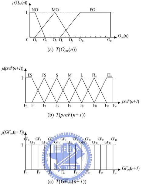
occupancy of CW/CCW ingress buffer in the end of the present agingInterval. Since FGFE is universal, here we take FGFE for CW ringlet for example. In order to reflect to tell the distinct levels of these parameters, we define the term sets of these input parameters as:
T(Ocw(n)) = { Normally Occupied (NO), More Occupied (MO), Fully Occupied (FO)}
T(preF(n+1))= {Extremely Small (ES), Pretty Small (PS), Small (S), Medium (M),
Large (L), Pretty Large (PL), Extremely Large (EL)}
The term “Normally Occupied” means that the STQ is in normal use. The term “More Occupied” shows the occupancy of the STQ is increasingly larger than STQ low threshold and the STQ is lightly congested. “Fully Occupied” indicates the usage of the STQ is over-utilized and it leads to packets loss easily. For a lower access delay and zero dropping probability, we hope the operation of STQ is in “Normally Occupied”. preF(n+1) is separated by seven terms. “Extremely Small” means the fair rate is closed to zero. “Extremely Large” represents the traffic scheduler in IGFC can serve CW or CCW ringlet buffer in nearly FULL_RATE. The remaining terms are averaged between “Extremely Large” and “Extremely Small”. Fuzzification of preF(n+1) just makes sure its position
and then we can adjust GF around the fuzzified value.
The membership functions of these terms should be defined with the proper shape and position. Generally speaking, a trapezoidal function or a triangular function is used to be the membership functions because they are suitable for real-time application. The two functions Tri x a b c and ( ; , , ) Trap x a b c d are given by ( ; , , , )
, , ( ; , , ) , , 0, , x a for a x b b a c x Tri x a b c for b x c c b otherwise − ⎧ < ≤ ⎪ − ⎪ ⎪ − =⎨ − < < ⎪ ⎪ ⎪⎩ (3.9) , , 1, , ( ; , , , ) , , 0, , x a for a x b b a for b x c Trap x a b c d d x for c x d d c otherwise − ⎧ < < ⎪ − ⎪ < < ⎪ = ⎨ − ⎪ < < − ⎪ ⎪ ⎩ (3.10)
where arguments, , , a b c in Tri(·) are three vertexes of the triangular function from left
to right; arguments, , , , a b c d in Trap(·) are four vertexes of the trapezoidal function
from left to right.
The membership functions associated with the terms NO, MO and FO in T(Ocw(n))
are (μNO O ncw( )), (μMO O ncw( )) and μFO(O ncw( )), respectively and are given by
0 0 1 3 ( cw( )) ( cw( ); , , , ) NO O n Trap O n O O O O μ = , (3.11) 1 5 8 ( cw( )) ( cw( ); , , ) MO O n Tri O n O O O μ = , (3.12) 6 10 16 16 ( cw( )) ( cw( ); , , , ) FO O n Trap O n O O O O μ = , (3.13) where 16 i sizeSTQ
O = ⋅ , i= 0, 1, …, 15, 16 and sizeSTQ is the total STQ size (bytes). i
LetμTerm(ser n( +1)) denote the membership functions for terms ES, PS, S, M, L, PL, EL in T(preF(n+1)) and define them as
0 0 1 3
( ( 1)) ( ( 1); , , , )
ES preF n Trap preF n F F F F
μ + = + , (3.14)
1 3 5
( ( 1)) ( ( 1); , , )
PS preF n Tri preF n F F F
μ + = + , (3.15)
3 5 7
( ( 1)) ( ( 1); , , )
S preF n Tri preF n F F F
μ + = + , (3.16)
5 7 9
( ( 1)) ( ( 1); , , )
M preF n Tri preF n F F F
μ + = + , (3.17)
7 9 11
( ( 1)) ( ( 1); , , )
L preF n Tri preF n F F F
μ + = + , (3.18)
9 11 13
( ( 1)) ( ( 1); , , )
PL preF n Tri preF n F F F
μ + = + , (3.19)
11 13 14 14
( ( 1)) ( ( 1); , , , )
EL preF n Trap preF n F F F F
μ + = + , (3.20)
where _ 14
i
FULL RATE
F = ⋅i, i = 0, …, 14 and FULL_RATE is link capacity (bytes/100μs). According to above defined fuzzy sets, the fuzzy rule is constructed in Table 4.1 that describes a fuzzy logic relationship in a form of “if-then” rules between 21 input linguistic variables and 15 output linguistic variables. Let Fi (i=0, 1, …, 14) also denote the i-th
level of the global fair rate estimation and define the term set of the output linguistic variables as T(GFcw(n+1))= {GF0, GF1, GF2, GF3, GF4, GF5, GF6, GF7, GF8, GF9, GF10,
GF11, GF12, GF13, GF14}. Then, the output membership functions are formulated as fuzzy
singletons which are uniformly distributed from 0 to FULL_RATE. That is, ( ( 1)) ( ( 1); , , ) i GF GF ncw Tri GF ncw F F Fi i i μ + = + , (3.21) where _ 14 i FULL RATE
F = ⋅i, i = 0,1, …, 14. Figure 3.6 shows the membership function of each fuzzy term set.
(a) T(Ocw(n))
(b) T(preF(n+1))
(c) T(GFcw(n+1))
Figure 3.6: The membership function of the term sets (a) T(Ocw(n)), (b) T(preF(n+1)), and
(c) T(GFcw(n+1))
FGFE acquires the two input linguistic terms from the fuzzifier and adopts the
max-min inference method to obtain the output linguistic term. In Table 4.1, for example,
rule 5th and rule 20th lead to the same result, GF3. For obtaining the output membership
values of “GFcw(n+1) is GF3”, the inference engine applies the min operation on
membership values of 5th and 20th rules, which are denoted as m5 and m20, respectively.
5 min( FO( cw( )), (S ( 1)))
m = μ O n μ preF n+ , (3.22)
20 min( NO( cw( )), (PS ( 1)))
m = μ O n μ preF n+ . (3.23)
value of control action “GFcw(n+1) is GF3” by 3 max( , )5 20 GF
M = m m . (3.24)
Similarly, the other fourteen ouput membership values of control actions:
0 GF M , 1 GF M , 2 GF M , 4 GF M , …, 13 GF M and 14 GF
M can be obtained. After inferring all rules, using the
center of area defuzzifcation strategy generates an overall GFcw as follows:
14 0 14 0 ( 1) i GF i cw i i i F M GF n F = = ⋅ + =
∑
∑
, (3.25)where Fi is the fuzzy singlton value corresponding to the output fuzzy term set.
Table 3.1: The rule base of fuzzy global fair rate estimator
rule Ocw(n) preF(n+1) GFcw(n+1) rule Ocw(n) preF(n+1) GFcw(n+1) rule Ocw(n) preF(n+1) GFcw(n+1)
1 FO EL GF12 8 MO EL GF13 15 NO EL GF14 2 FO PL GF10 9 MO PL GF11 16 NO PL GF12 3 FO L GF7 10 MO L GF9 17 NO L GF10 4 FO M GF5 11 MO M GF6 18 NO M GF8 5 FO S GF3 12 MO S GF4 19 NO S GF6 6 FO PS GF1 13 MO PS GF2 20 NO PS GF3 7 FO ES GF0 14 MO ES GF1 21 NO ES GF2
3.5 Traffic Scheduling
For fine control of output traffic and prevention of head of line blocking, two separate buffers are used to store inter-ring traffic from CW or CCW. Referred to Figure 3.1, the traffic scheduler is used to manage traffic between local, CW and CCW ingress buffers. Seeing that PTQ has higher priority than STQ, the three PTQs are scheduled first in round robin until they are empty. Per byte state machine in IEEE 802.17 has mentioned how to schedule from the STQ of local ringlet buffer (transit queue) to STQ of CW and CCW ingress buffers (add queue). It bases on round robin with some specified conditions. However, because the global fairness criteria are bandwidth fair share of IIA fairness eligible flows, the service rate of CW or CCW ingress buffer depends on how many IIA flows transit. Since there are variations in the number of IIA flows from time to time, the
dnamic weighted byte-by-byte round robin scheduling discipline is used. That is, every
agingInterval we observe how many IIA flows from CW or CCW direction arrive in IGFC, denoted by Numcw(n) in Eq. 3.2 and Numccw(n) in Eq. 3.3, respectively. Afterwards, the
STQ of CW ringlet buffer and the STQ of CCW ringlet buffer are served byte-by-byte on
Numcw(n) to Numccw(n) ratio. When bytes accumulate to a packet size, the same bytes
3.6 Transiving Global Fairness Packets
A local station receives a global fairness packet via the opposing ringlet. If the received global fair rate is smaller than local fair rate, inter-ring traffic is limited by global fair rate and intra-ring traffic still obeys local fairness mechanism. Otherwise, only local fairness algorithm is implemented. This property ensures the coexistence of local and global fairness. A local station continues to send GF to the upstream node neighbor.
Without virtual destination queues, Bridge can not control certain IIA flow. Once a bridge receives multiple global fairness packets from different bridges, it will choose the smallest GF between itself generated GF and the received GFs.
Chapter 4
Simulation Results and Discussions
4.1 Simulation Environment
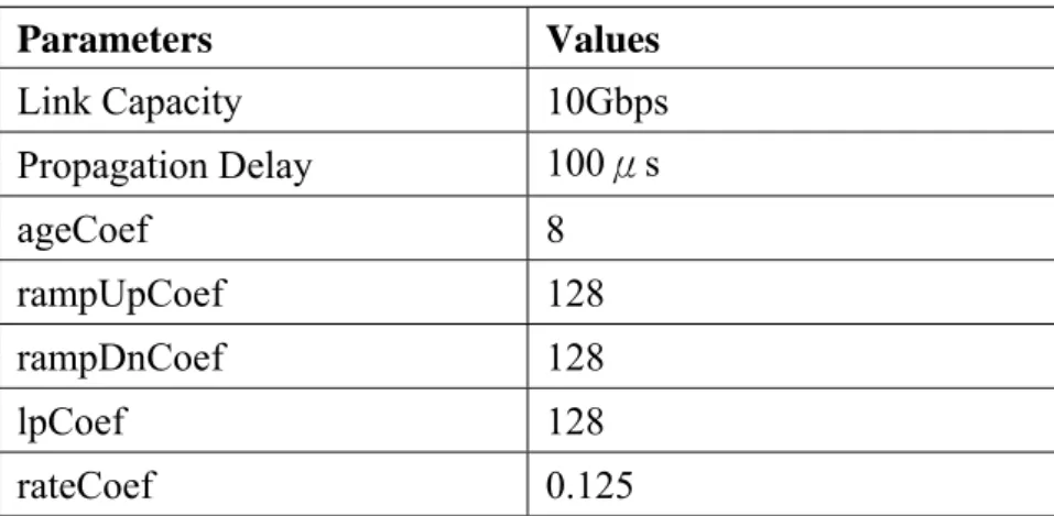
In this section, we compare our proposed intelligent global fairness controller (IGFC) with RIAS based global fairness controller (RGFC), [12]. The link capacity is 10Gbps (OC-192) and propagation delay between stations is 100μs. A uniform data packet is 1616 bytes and a fairness packet is 16 bytes. The agingInterval is 100μs and we observe and record the simulation result every agingInterval. We assume all traffic is best effort traffic. Some common parameters specified in IEEE 802.17 are regulated as Table 4.1.
Table 4.1: System Parameters
Parameters Values Link Capacity 10Gbps Propagation Delay 100μs ageCoef 8 rampUpCoef 128 rampDnCoef 128 lpCoef 128 rateCoef 0.125
We concentrate on a BRPR network with small and large topology scenario to justify the coexistence of global fairness and local fairness and to notice the influence of
propagation delay. For focusing on the transient behavior of inter-ring flows, we examine the dynamic traffic scenario which inter-ring flows start to transmit at different times. Unbalanced traffic scenario is concerned to realize what the weakness of AM leaves the global fairness controller and how IGFC fights against it.
We inspect the transmission rate of each source node to validate the global fairness criteria and the advantage of fair rate adjustment in fuzzy logic. The observation of throughput which is the received rate at the destination node can represent the gain of IGFC. Besides, dropping probability at bridge and averaged access delay at bridge are drawn to declare the significant system measure of IGFC by using fuzzy logic control. We do not perform the buffer overflow prevention scheme of RGFC, as described in chapter 1.4, since it is inadequate for supporting the real non-blocking quality of service. Here are the comparisons between IGFC and RGFC in Table 4.2.
Table 4.2: Comparisons between IGFC and RGFC
Elements and Attributions
IGFC RGFC
Ingress buffer 2 (4MB each) 1 (8MB)
Local ringlet buffer 1 (4MB) 1 (4MB)
Buffer management FIFO FIFO
Traffic Scheduling on ingress and local ringlet buffer
Obey per byte sate
machine in IEEE 802.17
Obey per byte sate machine in IEEE 802.17
Traffic Scheduling on ingress buffers
Dynamic weighted
round robin None (unnecessary)
Global congested detection None 1. Ingress buffer length
2. Received local fair rate
Global fair rates generator Global fairness criteria
+ Fuzzy control Global fairness criteria
4.2 Small Topology Scenario
Figure 4.1 (a) exhibits a simple BRPR network with 7 nodes, where node 0, 1 and 2 are located in Rk and node 3, 4, 5, and 6 are located in Rk+1. All nodes except node 6 will
transmit greedy traffic to node 6. Flow (0, 6), flow (1, 6), and flow (2, 6) are inter-ring traffic. Flow (0,6) and flow (1,6) are forwarded by CW ingress buffer and flow (2, 6) is forwarded by CCW ingress buffer of IGFC4. Flow (3, 6), flow (4, 6), flow (5, 6) are local
traffic. We want to inspect the affection of intra-ring traffic across the bridge, flow (3, 6) and flow (4, 6) which will transit through the local ringlet buffer of IGFC4.
(a) Scenario Setup
0 1000 2000 3000 4000 5000 6000 7000 8000
flow(0, 6) flow(1, 6) flow(2, 6)
flow(3, 6) flow(4, 6) flow(5, 6)
: : 0 10 20 30 40 50 60 70 80 90 100 (c) IGFC 0 1000 2000 3000 4000 5000 6000 7000 8000 0 10 20 30 40 50 60 70 80 90 100
flow(0, 6) flow(1, 6) flow(2, 6)
flow(3, 6) flow(4, 6) flow(5, 6)
: :
(d) RGFC
Figure 4.1: Small Topology Scenario. (a) Scenario Setup (b) Average Access Delay at Bridge, (c) IGFC, and (d) RGFC.
Figure 4.1 (b) shows the averaged access delay function of time to compare which controller has smaller access delay. We record the averaged access delay per 10ms and Y-axis is the number of agingInterval (100μs). Access delay is measured when a packet enter the buffer until it is served. It means a packet needs to be waited for the number of computational periods to being served. We can find that even if IGFC has two ingress
buffers, the access delay of CW or CCW ingress buffer of IGFC is very far smaller than RGFC’s. Arrival rate of each source node is not fully consistent because of propagation delay; in other words, it does not always match the current GF. When the total arrival rate has been larger than the available bandwidth for some agingIntervals, the buffer length increases and the buffer is inclined to overflow. RGFC with longer access delay means RGFC does not perform effective strategy to throttle buffer occupancy growing. Since the buffer occupancy is concerned into FGFE, IGFC provides the capability to adapt to system dynamics. Fortunately, both IGFC and RGFC do not occur buffer overflow because the defect of propagation delay does not appear apparently in small topology scenario. Upstream nodes can react to the bridge congestion and throttle their transmit rate fast. However, RGFC is close to buffer overflow.
Figure 4.1 (c) and (d) display throughput versus time by taking IGFC and RGFC, respectively. Both IGFC and RGFC not only successfully maintain local fairness but achieve global fairness. Intra-ring flow (3, 6), flow (4, 6), and flow (5, 6) all achieve 2.5Gbps; meanwhile, inter-ring flow (0, 6), flow (1, 6), flow (2, 6) equally share 2.5Gbps, which is 833.33Mbps each. The movements of local traffic by IGFC and RGFC are equivalent even if some intra-ring traffic is across the bridge. This is because AM local fairness algorithm is used in nodes and the bridge as well. If throughput is around 1.5% deviation of the ideal fair rate, we say that using the controller converges successfully in this scenario. Hence, the convergence time of IGFC for inter-ring traffic is 31ms, but the convergence time of RGFC for inter-ring traffic is 46ms. Even IGFC starts to be gradually stable after 20ms; nevertheless, RGFC is still unstable before 40ms. That is, using IGFC is better than RGFC at small topology scenario.
4.3 Large Topology Scenario
Propagation delay may postpone the convergence time and make severe oscillation since the far upstream nodes need to wait for more time until they receive the global fairness packet and limit their transmit rate. Therefore, we consider a large topology scenario, as illustrated in Figure 4.2 (a), where node 0, 1, 2, 3, 4, 5, and 6 are settled in Rk
and the other nodes are settled in Rk+1. All nodes except node 10 have infinite traffic
demands to node 10. Flow (7, 10), flow (8, 10), and flow (9, 10) are local traffic and the others are inter-ring traffic. Throughput, dropping probability, and transmission rate will be emphasized.
(b) Throughput by IGFC
(c) Throughput by RGFC
0 1000 2000 3000 4000 5000 6000 7000 8000
flow(0, 10) flow(1, 10) flow(2, 10) flow(3, 10) flow(4, 10) flow(5, 10) flow(6, 10)
:
0 10 20 30 40 50 60 70 80 90 100
(e) Transmission Rate of each source node by IGFC
(f) Transmission Rate of each source node by RGFC
Figure 4.2: Large Topology Scenario. (a) Scenario setup, (b) Throughput by IGFC, (c) Throughput by RGFC, (d) Dropping Probability at Bridge, (e) Transmission Rate of each source node by IGFC, and (f) Transmission Rate of each source node by RGFC.
Figure 4.2 (b) and (c) demonstrate throughput versus time by IGFC and RGFC, respectively. Regardless of intra-ring traffic, apparently, IGFC has better performance and stability than RGFC for inter-ring flows. The ideal global fair rate is 357.14Mbps and the ideal local fair rate is 2.5Gbps. IGFC trends to converge at 20ms and has a fast convergence time of 40ms, but RGFC has a slow convergence time of 54ms. In addition,
the variation of inter-ring flows by RGFC is more terrible and irregular. This is because too many distinct inter-ring flows enter the ingress buffer of RGFC. It is hard to manage all kinds of traffic due to first-in-first-out discipline plus the effect of propagation delay. In comparison with the last scenario, we can find that the propagation delay problem appears more terrible in large topology scenario, whether we focus on IGFC or RGFC. Since only the bridge computes GF and other nodes just propagate GF to their upstream node neighbor, for example, the bridge has to wait at least 10 round trip time to receive the reacting traffic of node 0 after the bridge has published the GF.
We record packets dropping probability at bridge every 100 agingIntervals in Figure 4.2 (d). Dropping probability is the number of dropped packets over transmitted packets during 10ms. Evidently, IGFC has zero packet loss; nevertheless, RGFC has at most 0.28 packet dropping probability. Fortunately, it does not occur buffer overflow after 20ms. The reason is that inter-ring traffic converges gradually and the congestion at bridge is solved. However, the utilization of the ingress buffer continues to be fully occupied and it is still not allowed because one of the BRPR targets is without packet loss.
Figure 4.2 (e) and (f) display the transmission rate of each source node, except node 7, 8, and 9. It is due to the same performance of local traffic. The observation at source nodes is eliminated from the damage of propagation delay as more as possible and is obvious if the GF was calculated correctly by the bridge. The convergence time of IGFC and RGFC is almost 26ms. However, IGFC adjusts with fewer and moderate oscillations, but RGFC adjusts with more and intense oscillations. It means IGFC can generate more precise GF. In RGFC, GF is only calculated according to the global fairness criteria. Unfortunately, when we face a large network, the remote nodes can not adapt their transmit rate as quickly as nodes close to the bridge. This makes the calculated GF is over
raised or reduced because of different arrival rate of each node. In IGFC, not only global fairness criteria but also the buffer occupancy alters the GF. We use fuzzy control to modulate GF since two ringlet buffers may store much enough data to serve out. Hence, fuzzy control is more sensitive and reflects to the real situation of the current network environment.
4.4 Dynamic Traffic Scenario
As illustrated in Figure 4.3 (a), node 0, 1, 2, and 3 are in Rk and the others are in Rk+1.
In this scenario, we want to study the transient behavior for inter-ring traffic. Node 1 and node 3 and node 4 start at 0s; node 0 starts at 50ms; node 2 starts at 100ms. All traffic demands are greedy. Our destination is node 5. Figure 4.3 (b) and (c) present throughput versus time by using IGFC and RGFC without ringlet selection, respectively. In other words, each inter-ring flow will choose the shortest path to forward. Otherwise, Figure 4.3 (d) also demonstrates throughput versus time by adopting IGFC with weighted ringlet selector (WRS) and each flow will decide a suitable path when it enters the bridge. We set α to 0.6, that is; to wit, traffic load is more important than distance.
0 1000 2000 3000 4000 5000 6000
flow(0, 5) flow(1, 5) flow(2, 5) flow(3, 5) flow(4, 5)
flow(3, 5), flow(1, 5) flow(0, 5), flow(3, 5), flow(1, 5)
flow(2, 5) 52ms 102ms 0 20 40 60 80 100 120 140 160 (b) IGFC (c) RGFC (d) IGFC with WRS
Figure 4.3: Simple Rate Changing Scenario. (a) Scenario Setup, (b) IGFC, (c) RGFC, and (d) IGFC with WRS.
Since the scenario only has a local traffic flow (node 4), and has symmetric and few inter-ring traffic flows, there are few oscillations and short convergence time with IGFC and RGFC. In Figure 4.3 (b), IGFC first converges to the ideal global fair rate at 56ms after node 0 begins to transmit traffic at 50ms; it second converges to the ideal global fair rate at 105ms after node 2 starts to transmit traffic at 100ms. In Figure 4.3 (c), the first convergence time by RGFC is 66ms and the second convergence time is 115ms. It can be found that using IGFC has a fast convergence time than using RGFC. The difference of convergence time is about 10ms which is 100 computation periods (agingInterval). This is because when node 0 or node 2 starts to transmit traffic, the ingress buffer of RGFC has keep much traffic and the destination node can not receive the new added traffic immediately.
IGFC has a great advantage on buffer management, but has some fluctuations while the traffic is changing. The reason is that scheduling between CW and CCW ingress buffers is measured by the dynamic weighted round robin. For example, CW and CCW ingress buffers are served at 2:1 ratio as flow (0, 5) reaches the bridge. Meanwhile, flow (0, 5) can not be served yet so flow (1, 5) has larger throughput. Similarly, flow (3, 5) fluctuates but flow (2,5) waits for being served around 100ms.
Figure 4.3 (d) reveals the advantage of using WRS. Inter-ring flows choose a suitable path according to Table 2.1. In the beginning, distance is the dominant factor and flow (1, 5) and flow (3, 5) are selected the shortest path (CCW) by SAS. Consequently, flow (1, 5) and flow (3, 5) are put into CW and CCW ingress buffer of IGFC4, respectively. As flow
Although transmitting traffic along the CW path is twice as far as the opposing path, traffic load dominates the decision at that time. Even though IGFC3 and IGFC4 generate
each GFcw and GFccw for node 0 and 1, and node 2 and 3, respectively, SAS would pick
the smaller GFcw and GFccw to ensure universal global fairness and broadcast them to
upstream nodes. It can be found that inter-ring flows make use of unused bandwidth. Hence, the total inter-ring traffic throughput by IGFC with WRS is twice more than IGFC without WRS.
4.5 Unbalanced Traffic Scenario
There is a problem with AM in RPR that permanent oscillations occur with low rate downstream flows and unbalanced traffic. Figure 4.4 (a) shows node 0, 1, 2, and 3 are in Rk and node 4 and 5 are in Rk+1. In this case, we assume flow (4, 5) is a lower rate
1.2Gbps for the sake of noting the action of greedy inter-ring traffic, flow (0, 5), flow (1, 5), flow (2, 5), and flow (3, 5) under the unbalanced traffic scenario. Since node 0 and node 1 are symmetric with node 2 and node 3, the former has the same uptrend and downtrend with the latter. So, we use blue line to represent flow (0, 5) and flow (2, 5); golden line to illustrate flow (1, 5) and flow (3, 5). The ideal global fair rate is 2.2Gbps per flow.
(a) Scenario Setup
(b) IGFC
(d) Dropping Probability at Bridge
Figure 4.4: Unbalanced Traffic Scenario. (a) Scenario setup, (b) IGFC, (c) RGFC, and (d) Dropping Probability at Bridge.
Figure 4.4 (b) and (c) illustrate throughput versus time by IGFC and RGFC, respectively. Regardless of using IGFC or RGFC leads to permanent oscillations under the unbalanced traffic scenario. This is because we apply AM as the local fairness algorithm. The maximum amount of traffic which nodes on Rk can output is subject to global fairness
but not themselves local fairness, since they are never locally congested. When node 4 is congested, it sends the local fairness control packet with LF of 1.2Gbps to the bridge. Accordingly, the available bandwidth for all inter-ring traffic is throttled to 1.2Gbps; moreover, node 0, 1, 2, and 3 decrease their add rate according to the adjusted GF. When the congestion at node 4 is resolved, it forwards LF of FULL_RATE to the bridge. Thus the bridge can transmit traffic as more as possible below the link capacity, and meantime upstream nodes can increase their add rate until congestion at node 4 takes place again to start another oscillation cycle. Therefore oscillations can not be eliminated.
However, it is obvious that using IGFC has moderate oscillations, but using RGFC has severe oscillations. Figure 4.4 (d) shows dropping probability at bridge in comparison with IGFC and RGFC. IGFC has immunity against buffer overflow, but RGFC has at
most 0.22 packet dropping probability. Since node 4 is periodically congested and the available inter-ring bandwidth is varied, the dropping probability by RGFC can not be eliminated and is also circulated. IGFC, composed of FGFE, provides a soft adaptive capability to avoid buffer overflow and generates an appropriate GF even under the disadvantageous scenario. It seems that the system with RGFC converges fast until the first ripple rises at 95th round in Figure 4.4 (c). It is an illusion because there is no congestion at node 4 before 95th round and the transmission rate of nodes on Rk is
FULL_RATE. Afterwards, congestion occurs at node periodically and it accompanies violent fluctuations. Figure 4.4 (c) exhibits a weird phenomenon. Node 1 and node 3 which are close to the bridge always oscillate upon the ideal GF after a period; on the contrary, node 0 and node 2 fluctuates below the ideal GF. This is because the number of dropping packets of node 0 and node 2 are larger than node 1’s and node 3’s. When flow (0, 5) and flow (1, 5) (or flow (2, 5) and flow (3, 5)) nearly converge, it means node 4 is not congested.
Chapter 5
Conclusions
In this thesis, we emphasize the importance of global fairness and buffer overflow prevention in a bridged RPR network (BRPR). The current local fairness algorithms can not support global fairness. Design of global fairness controller for BRPR is the major concern in this dissertation. We introduce the global fairness criteria, which are inherited from RIAS local fairness reference model, to ensure the equal share of each inter-ring ingress aggregated (IIA) flow from the available inter-ring traffic bandwidth. Therefore the intelligent global fairness controller (IGFC) is accomplished to realize global fairness for inter-ring traffic, to maintain local fairness for intra-ring traffic, and to prevent from buffer overflow.
There are dual ingress buffers with the dynamic weighted round robin scheduling. These designs can help reduce the drawback of FIFO discipline only with a single ingress buffer, accommodating inter-ring traffic from CW and CCW, and efficiently serve inter-ring traffic corresponding to the global fairness criteria. IGFC has a local ringlet buffer to contain intra-ring traffic from upstream local nodes and so does a local node. In order to be consistent with local stations, local fair rate at the IGFC is calculated from the forward rates of two ingress buffers.