適用於展頻時脈產生器之全數位鎖相迴路

國 立 交 通 大 學

電子工程學系 電子工程研究所

碩士論文

適用於展頻時脈產生器之全數位鎖相迴路

All-Digital Phase-Locked Loop for

Spread-Spectrum Clock Generator

研 究 生：蘇明銓

指導教授：周世傑 教授

適用於展頻時脈產生器之全數位鎖相迴路

All-Digital Phase-Locked Loop for

Spread-Spectrum Clock Generator

研 究 生：蘇明銓 Student：Ming-Chiuan Su

指導教授：周世傑 教授 Advisor：Prof. Shyh-Jye Jou

國 立 交 通 大 學

電子工程學系 電子工程研究所

碩士論文

A Thesis

Submitted to Department of Electronics Engineering & Institute of Electronics College of Electrical and Computer Engineering

National Chiao Tung University in partial Fulfillment of the Requirements

for the Degree of Master of Science in

Department of Electronics Engineering September 2009

Hsinchu, Taiwan, Republic of China

中華民國 九十八年 九月

適用於展頻時脈產生器之全數位鎖相迴路

研究生：蘇明銓

指導教授：周世傑 教授

國立交通大學

電子工程研究所碩士班

摘要

系統晶片中隨著內部參考時脈的提升，為了對抗電磁波干擾的問題，展頻技 術被應用在時脈的產生。傳統類比鎖相迴路較易受到製程/電壓/溫度變化的影響。 因此在使用深次微米互補式金氧半製程時，鎖相迴路遂逐漸向全數位式設計。 全數位鎖相迴路由bang-bang 相位頻率偵測器、使用累加器為主的數位迴路 濾波器、差動式數位控制震盪器和除頻器等組成。Bang-bang 相位頻率偵測器產 生相位比較訊號，控制使用累加器為主的數位迴路濾波器。然後，數位迴路濾波 器輸出粗調以及微調的控制碼，用以改變差動式數位控制震盪器的頻率。使用和 差調變器進一步控制數位控制震盪器可增加全數位鎖相迴路的頻率解析度。展頻 時脈的產生需要應用一個低抖動的全數位鎖相迴路。 展頻技術是對時脈信號的中心頻率做微量的調變，使時脈信號的頻譜展開成 較寬的頻帶範圍。因此可降低時脈信號在頻譜上的能量峰值，減少時脈信號所造 成的高頻電磁雜訊干擾(Electro-Magnetic Interference, EMI)。未來提出的時脈產生 器以全數位鎖相迴路為基本架構，可能使用和差調變器及調變多重相位的方法來 實現展頻，並且以符合Serial-ATA 6Gbps 的規格和 USB 3.0 5Gbps 的規格作為參 考設計。 展頻時脈產生器可依照系統對低功率需求或是對低抖動需求，選擇以10 個 輸出相位或是20 個輸出相位作展頻。本論文探討全數位鎖相迴路及展頻時脈產 生器的設計，以及使用TSMC 65nm 1P9M CMOS 製程的模擬。

All-Digital Phase-Locked Loop

for Spread-Spectrum Clock Generator

Student：Ming-Chiuan Su Advisor：Prof. Shyh-Jye Jou

Department of Electronics Engineering

Institute of Electronics

National Chiao Tung University

Abstract

As SOC(System On Chip) works with increasing internal reference clocks, the spread-spectrum clocking technique is used to mitigate EMI(Electro-Magnetic Interference) effect. Conventional analog PLLs are likely to be affected by PVT (process/voltage/temperature) variations. Hence, when using deep-submicron CMOS process, PLLs are prone to all-digital design.

All-digital PLL consists of bang-bang PFD, accumulator-based digital loop filter, differential DCO and divider. Bang-bang PFD generates phase compare signals to control accumulator-based digital loop filter. Then, DLF outputs coarse-tune and fine-tune control code to change differential DCO’s frequency. Using ΣΔmodulator to further control DCO enhances ADPLL’s frequency resolution. A low-jitter ADPLL is desired under spread-spectrum clocking application.

Spread-spectrum technique is to modulate clock’s center frequency, and the spectrum of the clock is spread over a broader range. Therefore, clock’s peak energy is reduced and it also mitigates EMI effect. Based on an ADPLL, the proposed spread spectrum clock generator (SSCG) is fulfilled usingΣΔmodulator and multiple phases. This SSCG uses Serial-ATA 6Gbps and USB 3.0 5Gbps specifications as reference.

For different system requirements for low-power or low-jitter, the SSCG can do modulation on 10 or 20 phases. The thesis proposes novel ADPLL and SSCG architecture and the circuits are implemented with TSMC 65nm 1P9M CMOS process.

致 謝

首先感謝周世傑老師在我這兩年多的碩士生涯中不遺餘力細心指導，經由一 次又一次的討論，使我慢慢累積一定程度的研究經驗以及學習如何研究的態度。 老師總是認真、用心的指導我的論文研究中可能有盲點的地方，也讓我在研究上 能更加進步。祝福老師身體健康，家庭幸福。在此也要感謝口試委員陳巍仁教授 以及蔡嘉明教授撥空參加口試，並能在口試中給予我寶貴的意見而能讓我的論文 更加完善。 再來要感謝我的父母，除了生活上讓我不虞匱乏，在學業上也是時時刻刻關 心我。因為有他們的照顧以及關懷，我在求學的路上能走的更平穩順遂，真的很 感謝我的父母。另外，也要感謝我的哥哥，在學習以及待人處事上總是給了我很 多意見，也是我一個學習的好榜樣。

接著，要謝謝所有在Mixed-Signal Circuit and System Lab的學長姐們，因為 有他們引導，讓我能很快融入這個大家庭。不管是在平常的哈拉當中或是在每次 的實驗室出遊或是邀約外出吃飯，都讓我跟實驗室成員彼此更佳的熟悉；有了他 們，研究的日子總是在歡樂當中度過。 最後，除了在碩士生涯的研究之外，我還想再更進一步提升自我研究能力。 未來也將繼續在這裡攻讀博士。也希望藉著在這個我熟悉的環境，能更快步上研 究軌道以及補強我不足的地方，並能再次學習更廣層面的課程！ 人生的路上都會遇上一些過客，能感謝的人太多了，不管是所有的授課老師 們、學長姐們、同學、學弟妹們，我也想同樣的感謝你們，有了你們的牽成，我 的學習生涯會更好，謝謝你們。 蘇明銓 于 新竹 國立交通大學 2009.09

Contents

1 Introduction

1

1.1 Background 1

1.2 Motivations and Goals 2

1.3 Thesis Organization 3

2 Spread-Spectrum Clocking

4

2.1 Background: EMI Problem 4

2.2 Concept of Spread-Spectrum 5

2.3 Phase Rotation Mechanism for Spread-Spectrum Clocking 7

2.4 ΣΔ Modulator 11

2.5 Timing Jitter Issue 15

2.6 Conclusions 17

3 All-Digital Phase-Locked Loop Basics

18

3.1 Introduction 18

3.2 All-Digital Phase-Locked Loop 19

3.2.1 Digitally-Controlled Oscillator 20

3.2.2 High Resolution Delay Cell 24

3.3 All-Digital PLL with Time-to-Digital Converter 26

4 Proposed All-Digital Phase-Locked Loop

28

4.1 Architecture Briefs 28

4.2 Phase Frequency Detector with Phase Threshold Detector 30

4.4 Differential Digitally-Controlled Oscillator 34

4.5 ΣΔ Modulator 38

4.6 Frequency Divider 42

5 Spread-Spectrum Clock Generator

44

5.1 System Architecture 44

5.2 ADPLL Behavioral Simulation 47

5.3 Circuit Implementation 50

5.3.1 PFD with Phase Threshold Detector 50

5.3.2 The 1st Order ΣΔ Modulator Design 51

5.3.3 Differential Digitally-Controlled Oscillator 53

5.3.4 Frequency Divider 59

5.3.5 ADPLL Summary 60

5.3.6 Triangular Wave Profile Generator 65

5.3.7 ΣΔ Modulator 67

5.3.8 MUX Control Circuit 68

5.3.9 Multiplexer 69

5.3.10 SSCG System 71

5.4 Measurement Setup 74

6 Conclusions and Future Work

76

List of Figures

Fig 1.1 High speed serial link block diagram 2

Fig 2.1 FFC class B EMI peak emission limit [4] 4

Fig 2.2 SSC frequency domain view 5

Fig 2.3 Triangular profile modulation 6

Fig 2.4 SATA-III triangular profile modulation [33] 7

Fig 2.5 Timing diagram of 10 phases from DCO 8

Fig 2.6 Timing diagram of phase rotation 8

Fig 2.7 Phase rotation ADPLL for spread-spectrum clocking 9

Fig 2.8 Periodic phase error accumulation phenomenon 10

Fig 2.9 Noise shaping for eliminating spurs induced by randomization 12

Fig 2.10 Waveform of d(t) 12

Fig 2.11 Architecture of 1st order ΣΔ modulator 13

Fig 2.12 Realization of ΣΔ modulator for phase rotation mechanism 13

Fig 2.13 Implementation of 2nd order ΣΔ modulator 14

Fig. 2.14 Clock’s Waveform in Time Domain (a) without frequency modulation (b) with frequency modulation 15

Fig 2.15 Cycle-to-cycle jitter diagram 15

Fig 2.16 Diagram of peak-to-peak jitter 17

Fig 3.1 Architecture of proposed ADPLL 20

Fig 3.2 Conventional DCO structure [9] 21

Fig 3.3 (a) DCO architecture in [10] and (b) fine-tuning delay cell in [10] 22

Fig 3.4 (a) DCO architecture in [11] and (b) fine-tuning delay cell in [11] 23

Fig 3.6 Differential delay cell [14] 25

Fig 3.7 TDC-based ADPLL [2] 26

Fig 3.8 Time-to-digital converter (TDC) [2] 27

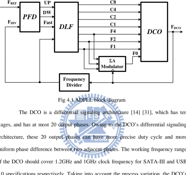
Fig 4.1 ADPLL block diagram 29

Fig 4.2 PFD architecture with tri-state PFD and phase threshold detector 30

Fig 4.3 PFD’s operation waveform to show the behavior of “Fast” 31

Fig 4.4 Digital loop filter architecture 32

Fig 4.5 DCO differential delay cell [14][31] 36

Fig 4.6 DCO architecture 36

Fig 4.7 DCO’s coarse tune and fine tune mechanism chart 38

Fig 4.8 ΣΔ modulator (a) general block diagram and (b) linear model 39

Fig 4.9 1st order ΣΔ modulator digital block diagram 40

Fig 4.10 Realization of 1st order ΣΔ modulator 41

Fig 4.11 Frequency divider 43

Fig 5.1 Architecture of spread spectrum clock generator 45

Fig 5.2 SIMULINK model of the proposed ADPLL 48

Fig 5.3 (a) The ADPLL’s output frequency V.S. time plot and (b) zoom-in plot 49

Fig 5.4 PFD simulation: “FREF” has higher frequency than “FDIV” 50

Fig 5.5 PFD simulation: “FDIV” has higher frequency than “FREF” 51

Fig 5.6 The 1st order ΣΔ modulator applied in ADPLL 52

Fig 5.7 Simulation plot of 1st order ΣΔ modulator 53

Fig 5.8 DCO‘s frequency V.S. coarse tune control code plot 54

Fig 5.9 DCO‘s frequency V.S. fine tune control code plot 55

Fig 5.11 DCO characteristic: frequency V.S. control code plot 56

Fig 5.12 DCO’s 20 output phases 57

Fig 5.13 (a) DCO’s peak-to-peak jitter and (b) zoom-in plot 59

Fig 5.14 Frequency divider simulation 60

Fig 5.15 (a) ADPLL’s DCO control words acquisition and (b) zoom-in plot 61

Fig. 5.16 ADPLL peak-to-peak jitter plot 62

Fig 5.17 Layout of proposed ADPLL 62

Fig 5.18 Triangular modulation profile generator 65

Fig 5.19 The 1st order ΣΔ modulator applied in SSCG 67

Fig 5.20 Programmable MUX control circuit 68

Fig 5.21 The 20 to 1 multiplexer 70

Fig 5.22 Carrier spectrum without spread spectrum (0dBV @ 1.2GHz) 71

Fig 5.23 Carrier spectrum with spread spectrum in (a) 10 phases SSCG and (b) 20 phases SSCG 72

Fig 5.24 Chip layout of proposed SSCG 73

List of Tables

Table 4.1 DCO’s output cycle variation under control of 1st order ΣΔ modulator 42

Table 5.1 SSCG design parameters 47

Table 5.2 DCO specification 58

Table 5.3 DCO frequency range with different corner 58

Table 5.4 ADPLL performance summary 63

Table 5.5 Comparison of ADPLL performance 64

Table 5.6 Parameters in programmable modulation profile generator 66

Table 5.7 Transforming equations of the control circuit 69

Table 5.8 SSCG layout attributes 73

Table 5.9 Programmable SSCG performance comparison 73

Chapter 1

Introduction

1.1 Background

PLL plays an important role in all kinds of integrated circuits, with the functions of frequency synthesis, duty-cycle correction, clock recovery and clock de-skewing. The realization of the PLL using a traditional analog architecture requires different demands on the process technology from those circuits using standard logic cells. Analog PLLs require elements that are not critical to standard logic circuits, such as resistors and low-leakage capacitors. In addition, analog PLL may use logic families like current mode logic other than static CMOS. With process evolves and grows in complexity, the challenge of maintaining performance for use in circuit increase dramatically. Furthermore, because the passive elements and logic families used by analog PLL are not likely to be reused by digital core, its yield and performance is worse as compared to those of the digital parts of the chip.

A number of all-digital PLLs have been proposed in the papers [10], [15], [18], [31], with target applications of fast lock-in time or low power. The major all-digital PLL design issues include phase error offset between reference and feedback divided clock, the algorithm of the fast lock-in process, the performance of digital loop filter, frequency resolution enhancement of digitally-controlled oscillator, and other critical concern like low-jitter and low-power considerations.

Modern high speed serial link is composed of a transmitter and a receiver and data are transmitted over different channels like PCB track, cable, fiber, etc, as shown in Fig 1.1. The transmitter generates a high bandwidth signal. A serious problem

associated with high speed serial link is electro-magnetic interference (EMI). Electrical devices operating at high speed result in EMI, and such EMI may interfere with the operation of its source circuit and other equipments adjacent to the EMI source. Since heavy metal shielding is not a low-cost option in the lightweight portable device, spread spectrum technique [28], [29], [36] has been frequently used for EMI reduction.

Data in Clock Channel TX CDR D Q Transmitter Receiver Data out

Fig 1.1 High speed serial link block diagram

1.2 Motivations and Goals

The demands on high data-rate and integration of modern high speed serial link activate the design of clock generator circuit being able to work at multi-Giga bits/s. The work of this thesis is motivated in two ways, one is to design a low-jitter all-digital PLL with working frequency of 1GHz or 1.2 GHz, and the other is to fulfill the spread-spectrum clocking technique referenced to Serial-ATA III(6Gbps data rate) and USB3.0(5Gbps data rate) specifications.

The proposed all-digital PLL is a PFD based all-digital PLL, with 10 or 20 phase outputs. A ΣΔ modulator is used to control DCO to enhance all-digital PLL frequency resolution. A low-jitter ADPLL is desired for spread-spectrum clocking application.

The goal of spread-spectrum clock generator (SSCG) is to design an all digital SSCG with small area and high EMI reduction.

1.3 Thesis Organization

Chapter 1 gives a brief introduction to the design demands of all-digital PLL and spread-spectrum clocking.

Chapter 2 describes spread-spectrum clocking theory. To reduce EMI effect, spread-spectrum clocking is used in wire-line communication. In this work, 1st order ΣΔ modulator is adopted for switching phase mechanism.

Chapter 3 reviews different kinds of all-digital PLL design. Digitally-controlled oscillator (DCO) is the most important block in all-digital PLL design. DCO is composed of delay cells. Chapter 3 will make comparisons of those delay cells claimed to have fine frequency resolution. Some all-digital PLL architecture are introduced like TDC-based all-digital PLL.

Chapter 4 brings up the proposed all-digital PLL. Initially, an overview of this all-digital PLL is discussed. Next, the components of the all-digital PLL are introduced. Phase frequency detector with threshold detector determines phase lead/lag condition and detects phase difference. Digital loop filter consists of accumulators and some logic cells. Differential digitally-controlled oscillator provides 10 or 20 output phases and has frequency range that covers 1GHz and 1.2GHz when process variation is considered. A divide-by-10 frequency divider is used. Finally, ΣΔ modulator is used to enhance the frequency resolution of DCO.

Chapter 5 shows the experimental results of the spread-spectrum clock generator and Chapter 6 draws a conclusion.

Chapter 2

Spread-Spectrum Clocking

2.1 Background: EMI Problem

All electronic devices operating at faster speed result in more Electromagnetic Interference (EMI). EMI emission can cause more electronic devices to interfere with each other and degrade their performance and operation. As the data rate of serial links increases, the clock source must increase its working frequency. Since frequency sources such as crystal oscillator, phase-locked loop frequency synthesizer or other clock generators are major sources of EMI in electric circuits, designers utilizing these above clock generation schemes must consider EMI effect.

The Federal Communications Commission (FCC) in the United States has regulation rules about the maximum power of EMI. The FCC’s regulation has been divided into Class A and Class B for the electronic products. Industrial applications use the FCC’s Class A regulation; while residential and consumer applications use the FCC’s Class B regulation. This certification shows the electronic device conforms to standards which limit the amount of EMI that one can produce.

Fig 2.1 shows a FCC Class B plot of power (dBµV/m) versus frequency (MHz) for the peak emission requirements (at 10 meters).

Nowadays, FCC regulations only pay attention to peak emission power at given frequency but not the average emission power over the given frequency spectrum. Therefore, one circuit designer should focus on reducing peak EMI emission at any given frequency within the spectrum.

Today, several methods are developed to solve EMI problem, like metal shielding, multi-layer printed circuit boards, special casing, passive components, pulse shaping, slew-rate control, layout technique, and the spread spectrum clocking.

Spread spectrum clocking (SSC) scheme modulates the given frequency of the clock source slightly and so the energy of the given frequency on the spectrum will be dispersed to a controllable small range. Hence, the peak emission power within the spectrum degrades, and the EMI effect is weakened. This method is most popular and is our subject in this thesis.

2.2 Concept of Spread-Spectrum

Spread spectrum clocking (SSC) slightly modulates the frequency of the clock so as to spread its power over a range of frequencies on the spectrum such that the average power emitted at a specified frequency is reduced as shown in Figure 2.2.

In general, spread spectrum clocking can be classified into three kinds of modulation modes: center-spread, up-spread and down-spread, which are based on the spreading frequency compared with nominal frequency. We adopt the down-spread mechanism according the specification of SATA-III and USB 3.0.

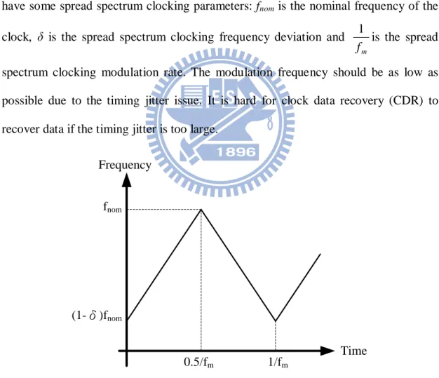
Fig 2.3 shows the triangular profile modulation in spread spectrum clocking. The triangular profile modulation will have the best EMI reduction because its frequency deviation is regular in a fixed time, so that the peak power of the spreading frequency can be reduced as a plane among the spectrum like that shown in Fig 2.2. Here we have some spread spectrum clocking parameters: fnom is the nominal frequency of the clock, δ is the spread spectrum clocking frequency deviation and

m

f

1

is the spread spectrum clocking modulation rate. The modulation frequency should be as low as possible due to the timing jitter issue. It is hard for clock data recovery (CDR) to recover data if the timing jitter is too large.

fnom

Frequency

Time (1-δ)fnom

0.5/fm 1/fm

Fig 2.3 Triangular profile modulation

A widely adopted SSC profile proposed in an industry standard, Serial AT Attachment (SATA) [33], is shown in Fig 2.4. We choose the nominal clock

frequency at 1.2GHz as the non-spread spectrum clocking frequency. The maximum spread spectrum clocking frequency deviation is 5000ppm and the modulation rate is 30~33 kHz as defined in SATA-III(6Gbps data rate) and USB 3.0(5Gbps data rate).

Fig 2.4 SATA-III triangular profile modulation [33]

As shown in Fig 2.3 the down spread technique is a way that the nominal clock frequency being moved below the nominal frequency between fnom and (1-δ) fnom, where δ is the maximum spread spectrum clocking frequency deviation with amount of 5000ppm down spread, and fm is modulation frequency of 30~33 kHz respectively.

2.3

Phase Rotation Mechanism for Spread-Spectrum Clocking

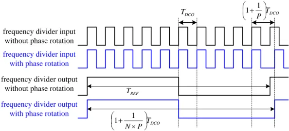
In this section, we will overview the static analysis of using phase rotation to achieve spread-spectrum clocking. Fig 2.5 shows the timing diagram of 10(P) phases from DCO. The phase difference between any two adjacent phases is the same.

If the period of each phase is TDCO, then the phase difference of two adjacent

phases is P T T T DCO DCO D = =

10 , where P is the number of phases provided by DCO. The output of DCO is fed into frequency divider which has a divide-ratio of N. The period of the frequency divider output without phase rotation is N×TDCO=TREF. If the input of

divider output will be _{DCO DCO} T_REF P N T N P N T P N ×      × + = × ×       × + = ×       + 1 1 1 1 1 . The timing diagram is shown in Fig 2.6.

phase0 phase1 phase2 phase3 phase4 phase5 phase6 phase7 phase8 phase9 TDCO TDCO/10

Fig 2.5 Timing diagram of 10 phases from DCO

DCO T P N      × + 1 1 REF T DCO T TDCO P     + 11 frequency divider input

without phase rotation

frequency divider input with phase rotation

frequency divider output without phase rotation

frequency divider output with phase rotation

As shown in Fig 2.6, the period of the output from the frequency divider with phase rotation is longer than that without phase rotation (TREF). When the output from

the frequency divider is sent back to the PFD, it will send out a “lag” signal so that the digital loop filter (DLF) will change the control code of the DCO which will speed up the DCO’s frequency, and the period of the frequency divider will decrease as well as the period of the DCO. The above mechanism is a transient behavior. When the ADPLL is stable, the period of the frequency divider’s output should be the same as TREF. Thus, the new TDCO must be less than the original TDCO under the same TREF.

This method can be used to vary the oscillation frequency of the DCO.

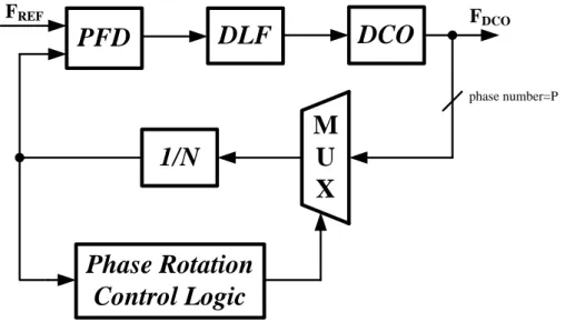
Fig 2.7 shows the basic architecture of the phase rotation ADPLL for spread-spectrum clocking. When the ADPLL is locked, the frequency divider has the

same frequency as FREF. And 

     × + × =       + × = P N F P N F

FDCO REF DCO original

α α

1

_ ,

where α is the phase rotation number. A multiplexer (MUX) is placed into the feedback path between the DCO and the frequency divider, and this MUX is controlled by phase rotation control logic circuit.

PFD

DLF

DCO

1/N

Phase Rotation

Control Logic

M

U

X

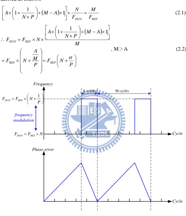
FREF phase number=P FDCO

For M sequence of FREF, if the MUX rotates one phase for A sequence and do not

rotate in the other (M-A) sequence, then the output frequency of the DCO can be derived as follows:

(

)

REF DCO F M F N A M P N A _× =      × − +       × + × 1 1 1 (2.1)

(

)

      + =           + × =       _{+ − ×}       × + × × × = ∴ P N F P M A N F M A M P N A N F F REF REF REF DCO α 1 1 1 , M＞A (2.2) Phase error Cycle Cycle Frequency       + × = P N F FDCO REF 1 N F F_DCO = _REF× frequency modulation A cycles M cycles

Fig 2.8 Periodic phase error accumulation phenomenon The equivalent rotation ratio is

M A

=

α . This value can vary between 0 and 1 by

is used. If we use counters to control the MUX, there is a periodic phase error accumulation phenomenon, as shown in Fig 2.8.

For the first (M-A) output pulses from the frequency divider, the MUX rotates no phase and the phase error accumulates. After MUX rotates one phase in “A” cycles, the phase error would be gradually compensated.

Since the phase error would yield phase rotation spurs per

M F_REF

offset from the carrier frequency, and such phase rotation spurs will decrease the quality of spread spectrum clock generator, it should be reduced as much as possible. The most popular method for solving this problem is to use the ΣΔ modulator. It will be explained in the next section.

2.4 ΣΔ Modulator

ΣΔ modulators are well widely used in communication and especially for A/D and D/A conversion applications. The objective of ΣΔ modulators is to shape the quantization noise spectrum such that a small amount of noise power remains within the useful signal band while the rest of the quantization noise pushed to higher frequency band.

In the previous section, the phase rotation spurs originate from the regular sequence of the MUX should be eliminated as much as possible. Hence, ΣΔ modulator can be used to randomize the choice of phase rotation while FDCO is still

given by       + × P N FREF α

as Eq. (2.2) shows. This means that individual multiplier factor occurs for only short period of time, the systematic fractional sideband would be converted to random noise. Further, one can shape the noise spectrum so that most of the noise’s energy could be moved to higher frequency offset. As a result, the noise in the vicinity of the FREF tone is adequately small. Moreover, the noise that is put into

high frequency offset can ideally be suppressed by the inherent low pass response of the ADPLL, as shown in Fig 2.9.

fREF fREF

f f

power power

Fig 2.9 Noise shaping for eliminating spurs induced by randomization

With the use of ΣΔ modulator [5], the phase-selection signal used to control the MUX has pseudo-random sequence and the quantization noise is differentiated in the signal band. The quantization noise results from that the phase-selection signal can only change from ith phase to (i+1)th phase but not fractional number, where i ranges from 0 to P-1 and P is the output phase number of DCO. Consequently, the ideal phase rotation of each selection is Y while it is quantized to either 0 or 1 (denoted as d(t)). Fig 2.10 shows one sequence example of d(t). Y is a time average value of d(t).

d(t) t 1 0 Y Fig 2.10 Waveform of d(t)

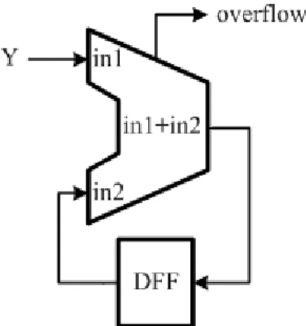
The implementation of ΣΔ modulator can be achieved by accumulator and D Flip-Flops (DFF). Fig 2.11 shows the architecture of the 1st order ΣΔ modulator.

Fig 2.11 Architecture of 1st order ΣΔ modulator The input normalized DC value of in1 is

M A A Y X = =

2 and the overflow is either 0 or 1, where A is the input of the accumulator, X is the bit number of the accumulator and M is the maximum number of the accumulator. As shown in Fig 2.12, the ΣΔ modulator’s overflow is sent to phase rotation control logic circuit to generate the phase-selection signal used to control the MUX for phase rotation mechanism.

PFD DLF DCO 1/N M U X Phase Rotation Control Logic DFF in1 in2 in1+in2 A FREF _FDCO phase number=P X overflow FDIV

For an X-bit accumulator, the accumulator would generate an overflow of average value A_X

2 at every FDIV clock. Therefore, the average number of phase

rotation is

(

)

P A A P A X X X × + = × − +       + × 2 1 2 1 2 1 1 .

In order to obtain better noise shaping toward higher frequency offset, the higher order ΣΔ modulator is required. Fig 2.13 shows the implementation of 2nd order ΣΔ modulator. DFF in1 in2 in1+in2 A overflow1 DFF in1 in2 in1+in2 DFF overflow2 -overflow

Fig 2.13 Implementation of 2nd order ΣΔ modulator

Here we use 1st order ΣΔ modulator to control the number of phase rotation. The reason of choosing 1st order ΣΔ modulator but not higher order ΣΔ modulator is that SATA-III specification must have down spread frequency modulation. The output of 2nd order ΣΔ modulator are -1, 0, 1, 2, and the “-1” term will have up spread frequency modulation even though the average is down spread. All of them could not plus 1; otherwise, much more jitter would be produced. For example, if the original

output is 2, it would become 3 after it adds 1. It means that MUX will rotate 3 phases in one PFD comparison, so the spread spectrum modulation deviation would be

ppm P N 10 20 15000 3 = × = × α

and is beyond the scope.

2.5 Timing Jitter Issue

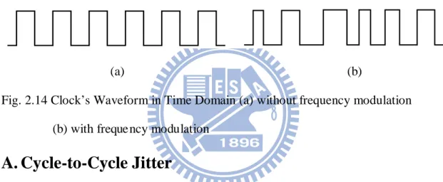
In the SSCG system, the output frequency is spread over time. If the transmitter uses the SSCG system to generate the clock, then the data is affected by the clock’s performance. For example, as shown in Fig 2.14, the clock’s waveform would vary over time.

(a) (b)

Fig. 2.14 Clock’s Waveform in Time Domain (a) without frequency modulation (b) with freque ncy modulation

A. Cycle-to-Cycle Jitter

The cycle-to cycle jitter can vary over time, because its measurement depends on the relationship between the present cycle time and the previous cycle time. Fig 2.15 shows the relationship between cycle time and jitter.

Time Amplitude

T1 T2 T3

Jitter1_2=T1-T2 Jitter2_3=T2-T3

Below we derive the formulas about cycle-to-cycle jitter. The period difference between the normal frequency and the maximum modulated frequency is:

(

)

normal normal

(

)

normal normal total f f f f T δ δ δ δ − = − ≈ − = ∆ 1 1 1 1 (2.3)

δ is the frequency modulation deviation, and fnormal is the normal frequency.

The number of cycles (N) that exists in the time interval that the modulated clock moves from fnormal to (1-δ) fnormal is:

m avg f f N 2 = (2.4)

Where favg is the average frequency of the spread spectrum clock, and fm is the modulated frequency. According to triangular modulation profile, we could derive the average frequency as

(

)

normal

avg f

f = 1−0.5δ (2.5) Therefore, the cycle-to-cycle jitter induced from spread spectrum clock can be expressed as

(

)

(

)

2 5 . 0 1 2 5 . 0 1 2 normal m normal m normal total cycle to cycle f f f f f N T T δ δ δ δ − = − ⋅ = ∆ = ∆ _{− −} (2.6)

For a 1.2GHz spread spectrum clock with 0.5% triangular modulation and 31.25 KHz modulation frequency, the cycle-to-cycle jitter is:

(

)

(

)

( )

fs T_{cycle to cycle} 2.175578 10 0.218 10 2 . 1 % 5 . 0 5 . 0 1 % 5 . 0 10 25 . 31 2 16 2 9 3 ≈ × ⋅⋅ ⋅ = × × × − × × × = ∆ − − − (2.7)

B. Long-Term Jitter

Long-term jitter measures the maximum change in a clock’s output transition from its ideal position. Fig 2.16 shows the diagram of peak-to-peak jitter. As a result, equation (2.3) can be viewed as the long-term jitter of a down-spreading clock.

Analogously, for a 1.2GHz spread spectrum clock with 0.5% triangular modulation and 31.25 KHz modulation frequency, the long-term jitter is:

( )

ps f T normal total 4.166 10 4.2 10 2 . 1 % 5 . 0 12 9 = ⋅ ⋅⋅× ≈ × = = ∆ δ − _(2.8) Time Amplitude Time Amplitude Jitter ideal clock real clock

Fig 2.16 Diagram of peak-to-peak jitter

2.6 Conclusions

In this chapter, we introduce the EMI problem and spread-spectrum clocking is used to reduce the EMI. Phase rotation mechanism is applied to the proposed ADPLL to construct the spread-spectrum clock generator (SSCG). The SSCG can turn on or turn off its spread-spectrum clocking under the “switch” signal. Also, the SSCG can choose 10 phases or 20 phases spread-spectrum clocking under the “select” signal. Our goal is to design an all-digital SSCG with small area, less power consumption and good EMI reduction.

Chapter 3

All-Digital Phase-Locked Loop Basics

3.1 Introduction

Phase-locked loops (PLLs) have been used in different kinds of IC for many years. PLLs are widely used in frequency synthesis and timing recovery filed, especially for the serial link transceiver.

To date, most PLLs are analog feedback circuits that have a particular system to track with reference signal. In other words, PLLs generate an output clock that is synchronized with a reference clock in frequency as well as in phase. Once the PLLs are locked, the phase error between the frequency divider output clock and the reference clock is ideally zero.

The main applications of PLL are as follows:

1. Clock generation: Most electronic systems have processors operating at various clock frequencies. PLLs serve to provide them with clock frequency. Usually, a lower reference clock frequency (usually 50 or 100 MHz) is multiplied by N (multiplication factor), so as to generate a higher operating frequency the processor needs. The multiplication factor can be an integer or a fractional number.

2. Spread spectrum: Electronic devices working at high frequency will emit some unwanted electro-magnetic wave. Such emitted electro-magnetic wave generally appears as sharp spectral peaks (usually at the device’s working frequency, and its harmonics). For an economic way to reduce EMI, PLLs are modified for spread-spectrum clocking. By spreading the sharp spectral peak energy over a wider portion of the spectrum, the EMI problem is released. For example, by changing the

operating frequency up and down by a small amount (about 1%), a device running at hundreds of megahertz can spread its interference evenly over a few megahertz of spectrum, which drastically reduces the amount of noise seen by FM receivers which have a bandwidth of tens of kilohertz.

3. Clock recovery: Some data streams, especially high-speed serial data streams, (such as the raw stream of data from the magnetic head of a disk drive) are sent without an accompanying clock. The receiver generates a clock from an approximate frequency reference, and then phase-aligns to the transitions in the data stream with a PLL. In order for this scheme to work, the data stream must have a transition frequently enough to correct any drift in the PLL's oscillator. Typically, some sort of redundant encoding is used; 8B10B is very common.

4. De-skewing: If a clock is sent in parallel with data, that clock can be used to sample the data. Because the clock must be received and amplified before it can drive the flip-flops which sample the data, there will be a finite, and process-, temperature-, and voltage-dependent delay between the detected clock edge and the received data window. This delay limits the frequency at which data can be sent. One way of eliminating this delay is to include a de-skew PLL on the receive side, so that the clock at each data flip-flop is phase-matched to the received clock.

3.2 All-Digital Phase-Locked Loop

Many kinds of all-digital PLLs are presented so far, and some are suitable for specific applications. When well-controlled bandwidth is required for wireless applications, a high resolution time-to-digital converter (TDC) [6] with multi-bits is used. For the requirement on short lock times, a delicate digital search algorithm and a control scheme may be needed [7]. Fast lock-in time can also be achieved by the use of dual-loop architecture [8] (one loop for frequency acquisition, and the other for

phase alignment) with different loop filter characteristics to support frequency and phase acquisition, respectively. The above architectural choices significantly increase area, power consumption and circuit complexity without commensurate benefit for the clock generation application described here.

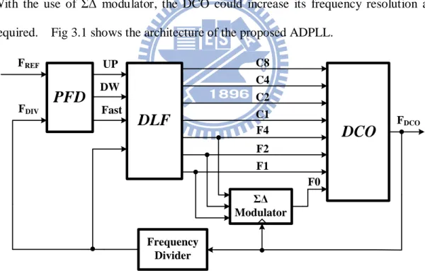
The proposed all-digital PLL is designed for spread-spectrum clock generation, and in this application, the critical specification is peak to peak period jitter. The realized ADPLL uses single loop architecture, based on a bang-bang phase/frequency detector (bang-bang PFD). Since no fast frequency hopping is required, this work does not acquire a high resolution multi-bit TDC. The proposed DCO has differential signaling, which has at most 20 phases for requirement on spread-spectrum clocking. With the use of ΣΔ modulator, the DCO could increase its frequency resolution as required. Fig 3.1 shows the architecture of the proposed ADPLL.

PFD

UP

DLF

DCO

ΣΔ Modulator DW Fast C8 C4 C2 C1 F4 F2 F1 F0 Frequency Divider FREF FDIV FDCO

Fig 3.1 Architecture of proposed ADPLL

3.2.1 Digitally-Controlled Oscillator

The most critical component of the ADPLL is no doubt the digitally-controlled oscillator (DCO). It is impossible for the DCO to be realized in an ADPLL with extremely poor noise performance under free-running condition. Also, the tuning

range and the number of frequency control bits decide the DCO’s performance in a low-jitter ADPLL design.

Conventional DCO is composed of odd number of inverting cells, as shown in Fig 3.2. When changing its turn-on number of inverters, the DCO can change the path’s driving ability [9], so as to change its delay time as well as frequency. It has the advantage of using all-digital standard cells. But, it has limited frequency resolution and it is not suitable for high-frequency circuit application.

. . . M U X Delay Matrix Coarse-Search commands Fine-Search commands clock output EN0 EN1 EN2 ENn

Fig 3.2 Conventional DCO structure [9]

Another DCO has two control parts, as shown in Fig 3.3(a) [10]. One is coarse tune part and is composed of a group of delay. The other is fine tune part, which is designed for enhancing the DCO’s frequency resolution, as shown in Fig 3.3(b). By choosing different number of delay stages, DCO can change frequency. Using digital code to control the turn-on or turn-off conditions of the tri-state buffers, the delay time of the ring DCO can determine its oscillating frequency. However, once the inverter

delay time in a fine tune stage is the finest resolution delay time that the DCO can have, the DCO could not have very precise frequency.

P0

D[0] D[1] D[14]

EN[N-1] EN[N-16]

P1 P2 P(N/16-1)

FINE-TUNE OUT_CLK

SEP[(N/16)-1] SEP[(N/16)-2] SEP[(N/16)-3] SEP[0]

(a) IN A1 B1 EN1 1 A2 B2 EN2 1 OUT AOI OAI (b)

MUX

(multi-stage tri-state buffers)

Decoder Decoder Reset DCO code[13:8] Decoder DCO code[7:0] Coarse-Tuning Stage Fine-Tuning Stage (a) F_OUT

F1ON[0] F1ON[1] F1ON[7]

F2ON[0] F2ON[24] F2ON[31] F2ON[1] F2ON[25] F2ON[7] 1st Fine-Tune 2nd Fine-Tune F_IN (b)

Fig 3.4 (a) DCO architecture in [11] and (b) fine-tuning delay cell in [11] The coarse tune part is used to increase adjustable frequency range, so the delay cells in the coarse tune stage may have larger delay time as compared to fine tune

stage. The fine tune stage serves to enhance frequency resolution; therefore, the delay cells in fine tune stage need smaller delay time as possible.

Essentially, there are two main kinds for designing fine-tuning delay cell. One method is to change the path’s driving strength dynamically with a fixed capacitance loading. The other method is to change the effective loading capacitance so as to have fine-tuning ability [11], [12], [13]. Fig 3.4(a) is the DCO architecture and Fig 3.4(b) is its fine-tuning delay cell.

3.2.2 High Resolution Delay Cell

To apply ADPLL into higher frequency systems, designing a high resolution delay cell is essentially required. In an analog delay cell, the delay time which is controlled by its operating current or voltage is a continuous-time parameter. Nevertheless, in a digital delay cell, the delay time is quantized. The ADPLL could have smaller timing jitter if the DCO could achieve as more precise frequency resolution as possible. Some examples of digital high resolution delay cell are introduced below.

One digital realization of high resolution delay cell, as shown in Fig 3.3(b), is combined by one And-Or-Inverter (AOI) cell and one Or-And-Inverter (OAI) cell [10]. The usage of two parallel tri-state inverters is to increase the delay cell’s adjustable frequency range. Upon using the AOI and OAI cells can have the advantage of precisely changing delay cell’s driving ability and thus can improve delay time control, but with a disadvantage of being more sensitive to power-supply variation.

Another digital realization of high resolution delay cell, as shown in Fig 3.5 [12], uses the concept of changing the number of turn-on or turn-off loading cells between inverting cells in a DCO so as to change its effective loading capacitance as well as

the delay time. Due to tiny capacitance quantity change, such DCO could have resolution smaller than 1ps and more linear DCO characteristic (digitally controlled word vs. frequency range). For the sake of using of many loading transistors, the nodes within DCO may have large effective capacitance and result in large area and power consumption.

DCO_OUT

F1ON[0] F1ON[1] F1ON[P-2]

F2ON[0] F2ON[Q-P+1] 1st Fine-Tune 2nd Fine-Tune F_IN F1ON[P-1] Delay Path F2ON[0] F2ON[Q-P+2] F2ON[P-2] F2ON[Q-1] F3ON[0] F3ON[R-1] 3rd Fine-Tune

Fig 3.5 DCO fine tune stage in [12]

Vc

Vc Vin+

Vin- Vout+

Vout

-Fig 3.6 Differential delay cell [14]

In order to operate the DCO with higher frequency and have multiple phase outputs, we often use differential input/output delay cell to build a DCO [14]. As shown in Fig 3.6 is the differential delay cell. Differential input/output delay cell can construct a DCO without considering an odd or an even number of delay cells that should be used. Therefore, an even number of multiple phase outputs can be achieved.

3.3 All-Digital PLL with Time-to-Digital Converter

Fig 3.7 shows the TDC-based ADPLL block diagram from [2]. The ADPLL uses the time-to-digital converter (TDC) to detect not only the phase lead/lag information but also the phase difference between the reference clock and the feedback clock. Also, the phase difference is quantized into digital codes and these digital codes are sent to the cascaded digital loop filter, which is designed case by case. Then the digital loop filter manipulates one set of new DCO control words to control the DCO. This ADPLL features faster dynamics and is used where fast frequency and phase acquisition are required.

Fig 3.7 TDC-based ADPLL [2]

Fig 3.8 shows the time-to-digital converter from [2]. The TDC has quantized phase detector with resolution of 20ps. The DCO sends a clock and it passes through the inverter chain. Then, the delayed outputs are sampled by reference clock and generate a group of digital codes.

Because the TDC’s finest resolution decides the minimum phase difference that the ADPLL can detect, the delay inverters and DFFs need to be designed carefully.

Fig 3.8 Time-to-digital converter (TDC) [2]

The TDC’s design can be affected by the DCO frequency and the delay of the inverters in TDC. When the DCO frequency decreases (which means the period of DCO clock increases) and the delay of inverters in TDC is constant, then the number of inverters needed by TDC’s delay chain should increase for the sake of covering one full DCO clock cycle. Increasing the number of delay chain inverters can increase the TDC’s power consumption. Furthermore, when the inverter delay decreases, the TDC can have less quantization noise; however, the number of inverters needed by TDC’s delay chain should increase for the sake of covering one full DCO clock cycle and this can also increase TDC’s power consumption.

Chapter 4

Proposed All-Digital Phase-Locked

Loop

4.1 Architecture Briefs

Fig 4.1 shows the architecture of the proposed low-complexity ADPLL. This work is simply composed of phase/frequency detector (PFD), digital loop filter (DLF), frequency divider and the digitally-controlled oscillator (DCO). A ΣΔ modulator is used so that the DCO can have more precise frequency resolution. The DCO can have at most 20 phase outputs as needed by spread-spectrum clocking.

Based on SATAIII (data rate: 6Gbps) or USB3.0 (data rate: 5Gbps) specifications, the ADPLL should be able to lock at 1.2GHz or 1GHz clock frequency, which shall have 5 phases to reach the so-called data-rate. The divider ratio is 10 and is determined according to the spread spectrum clocking modulation deviation.

The phase/frequency detector (PFD) can not only detect the phase difference information (phase lead or phase lag) between the reference clock (FREF) and the

feedback clock (FDIV) but can also detect the phase difference extent and represent

this condition using one control bit, “Fast.” This seems like a one-bit time to digital converter.

After each comparison in PFD, the DLF is sampled by “FDIV” clock and changes

its control bits (C8, C4, C2, C1, F4, F2, and F1) based on the latest information (UP, DW, and Fast). The three fine-tune bit, F4, F2, and F1 are sent into 1st order ΣΔ modulator, which is sampled by “FDCO” clock, to generate one dithering bit, F0.

Totally, there are 8-bit control codes to the DCO and dominate its oscillation frequency.

PFD

UP

DLF

DCO

ΣΔ Modulator DW Fast C8 C4 C2 C1 F4 F2 F1 F0 Frequency Divider FREF FDIV FDCO

Fig 4.1 ADPLL block diagram

The DCO is a differential signaling architecture [14] [31], which has ten stages, and has at most 20 output phases. Owing to the DCO’s differential signaling architecture, these 20 output phases can have more precise duty cycle and more uniform phase difference between two adjacent phases. The working frequency range of the DCO should cover 1.2GHz and 1GHz clock frequency for SATA-III and USB 3.0 specifications respectively. Taking into account the process variation, the DCO’s frequency range should be large enough to overcome all process corners.

All the component blocks in the proposed ADPLL are built from digital logic cells, and through the customized design, this ADPLL can reach the low-complexity goal. Finally, the peak-to-peak period jitter and the power consumption are two main issues in the proposed ADPLL design.

4.2 Phase Frequency Detector with Phase Threshold

Detector

Fig 4.2 shows the PFD architecture. The PFD is composed of a conventional tri-state PFD and a phase threshold detector [15]. This PFD acts as the traditional PFD would be.

Q1

Q2

Fig 4.2 PFD architecture with tri-state PFD and phase threshold detector Initially, the “UP” and “DW” signals are both “0”.

If the reference clock’s rising edge (FREF) comes first, then the “UP” signal will

become “1”. Then when the divided clock’s rising edge (FDIV) comes, the “DW”

signal will also become “1”. Upon this condition, the PFD’s DFFs will be reset and the “UP” and “DW” signals will return to “0”.

Oppositely, if the divided clock’s rising edge (FDIV) comes first, then the “DW”

“UP” signal will also become “1”. Similarly, the PFD’s DFFs will also be reset and the “UP” and “DW” signals also return to “0” again.

The above operations of the PFD are inadequate in the lock-in process of the ADPLL. Because these operations only indicate the phase lead or lag information and are unable to show the extent of the phase difference. As a result, a phase threshold detector is added to the PFD to indicate the phase difference extent.

FREF FDIV UP DW Q1 Q2 Fast

Fig 4.3 PFD’s operation waveform to show the behavior of “Fast”

The proposed ADPLL has coarse tune codes and fine tune codes in DCO. In order to use coarse tune codes for the frequency acquisition and fine tune codes for the phase acquisition of the ADPLL, a phase threshold detector is applied in the PFD to generate a “Fast” signal to enable freque ncy acquisition to enhance the lock-in time. “Fast” signal becomes tunable when the phase difference between FREF and FDIV is

beyond ±π, as shown in Fig 4.3. In the next section, the usage of the “Fast” signal will be explained.

In the phase threshold detector, the “UP” and “DW” signals are sampled at the falling edges of the reference clock (FREF) and the divided clock (FDIV) respectively.

The sampled results are Q1 and Q2 respectively. These two signals are sent to the “OR” gate to generate the “Fast” signal.

4.3 Digital Loop Filter Design

Fig 4.4 shows digital loop filter architecture. The digital loop filter has three inputs: UP, DW and Fast. It generates 4-bit coarse tune codes: (C8, C4, C2, C1) and 3-bit fine tune codes: (F4, F2, F1). These control codes are sent into the DCO to generate the necessary oscillating frequency.

M U X UP DW 0 -1 1 0 Fast D Q FDIV in1 in2 in1+in2 D Q FDIV 4 4 Coarse-tune codes (C8, C4, C2, C1) M U X UP DW 0 1 -1 0 Fast D Q FDIV in1 in2 in1+in2 _{D Q} FDIV 3 3 Fine-tune codes (F4, F2, F1) overflow

Fig 4.4 Digital loop filter architecture

Initially, the digital loop filter sets a condition that the DCO can work at one frequency that is near its mid-frequency. There are basically two procedures for the digital loop filter to generate the coarse tune codes and fine tune codes. These two procedures are controlled by “Fast” signal.

According to the DCO’s characteristics in the next section, the larger coarse tune codes the DCO has, the higher oscillating frequency the DCO generates. On the other hand, the larger fine tune codes the DCO has, the lower oscillating frequency the DCO generates.

Under different conditions, the digital loop filter will operate differently as described below. One procedure is coarse tuning mechanism, or it may be called the “frequency acquisition.”

When “Fast” signal is high, the digital loop filter changes coarse tune codes (C8, C4, C2, C1) and maintains fine tune codes (F4, F2, F1) under the following situations: 1. When UP=1 and DW=0increase coarse tune code by 1

2. When UP=0 and DW=1decrease coarse tune code by 1 3. Others  coarse tune code holds

The above operations occur when the divided frequency (FDIV) from the

frequency divider and the reference frequency (FREF) sent into the PFD are quite

different and have phase difference more than ±π. Under this situation, the digital loop filter should change the coarse-tuning codes immediately so that the divided frequency (FDIV) from the frequency divider can be almost the same as the reference

frequency (FREF).

At the end of coarse tuning procedure, we assume that the divided frequency (FDIV) and the reference frequency (FREF) sent into the PFD shall have only slightly

frequency difference and this can be viewed to be the phase difference.

Next, the procedure is fine tuning mechanism, or it may be called the “phase acquisition.”

When “Fast” signal is low, the digital loop filter maintains coarse codes (C8, C4, C2, C1) and changes fine codes (F4, F2, F1) under the following conditions:

1. When UP=0 and DW=1increase fine tune code by 1 2. When UP=1 and DW=0decrease coarse tune code by 1 3. Others  fine tune code holds

The above operations occur when the divided frequency (FDIV) from the

frequency divider and the reference frequency (FREF) sent into the PFD have quite the

same frequency value and have phase difference within ±π. Under this situation, the digital loop filter should change the fine-tuning codes so that the phase difference between the divided frequency (FDIV) and reference frequency (FREF) can be

eliminated gradually.

At the end of fine tuning procedure, we assume that the divided frequency (FDIV)

and the reference frequency (FREF) sent into the PFD shall have only slightly phase

difference. Ultimately, the ADPLL can be in lock-in state when frequency acquisition and phase acquisition are done step by step. But one inherent drawback of the ADPLL is that the DCO of the ADPLL can only have certain discrete frequency under these coarse tune codes and fine tune codes combinations.

Since the proposed ADPLL is used for the application of spread spectrum clocking, the issue of low jitter performance of the proposed ADPLL is quite important. Therefore, due to limited frequency resolution of the DCO, we adopt a 1st order ΣΔ modulator to enhance the DCO’s frequency resolution. By way of using the 1st order ΣΔ modulator to enhance DCO’s frequency resolution, the proposed ADPLL can have better jitter performance.

4.4 Differential Digitally-Controlled Oscillator

The proposed ADPLL is used in spread spectrum clock generator, thus the number of ADPLL’s output phases is an important parameter for spread spectrum clocking. In the DCO design, we utilize the differential delay cell to construct a ten

stage DCO with differential outputs. Furthermore, the design of the control codes of the DCO is another important issue in ADPLL design. Finally, we should take care of the DCO’ output frequency range under the effects of process variation.

Fig 4.5 shows the DCO’s differential delay cell [14] [31] and Fig 4.6 shows the ten-stage architecture of the DCO. The coarse tune signals (C8, C4, C2, C1) control a couple of parallel tri-state inverters, whose on-off state would determine the differential delay cell’s driving strength. While the fine tune signals (F4, F2, F1) control a group of tri-state inverter based latches, whose on-off state would determine the differential delay cell’s loading quantity. The dithering-bit (F0) generated by ΣΔ modulator is used to control the first stage of the DCO and the rest 9 stages of the DCO have their F0 connected to ground so as to enhance the DCO’s frequency resolution.

The parallel driving cells with control-bit (C8, C4, C2, C1) are combined with the driving cell as shown in Fig 4.5; also, the loading cells with control-bit (F4, F2, F1) are connected with one loading cell. The advantage of using differential cell is that each stage of the DCO can have differential outputs and each stage’s output can have good duty cycle performance. Differential architecture of the DCO can make its output’s number to be double the DCO’s stage number. Furthermore, the good duty cycle performance of each output from the DCO that results from differential architecture is important for switch phase mechanism used in spread spectrum clocking.

C8 C4 C2 C1 M2=8 M2=4 M2=2 M2=1 Vin+ driving cell M2=16 F4 M1=4 F2 M1=2 F1 M1=1 F0 M1=1 C8 C4 C2 C1 M2=8 M2=4 M2=2 M2=1 Vin -driving cell M1=24 Vout -Vout+ loading cell Vin+ Vin -Vout -Vout+ coarse-tune code fine-tune code M2=16

Fig 4.5 DCO differential delay cell [14] [31]

Vin+ Vin -Vout -Vout+ coarse-tune code (C8, C4, C2, C1) fine-tune code (F4, F2, F1) Vin+ Vin -Vout -Vout+ Vin+ Vin -Vout -Vout+

stage1 stage2 stage10

dithering-bit (F0)

The stronger the parallel driving cells’ driving strength is, the smaller delay time the differential delay cell has. These parallel driving cells are served to be coarse tuning cells. Hence, the higher the coarse tune codes are, the stronger the driving strength is and as well as the higher oscillating frequency. On the opposite, the smaller the coarse tune codes are, the weaker the driving strength is and as well as the lower oscillating frequency.

The less the loading latches are turned on, the smaller delay time the differential delay cell has. These parallel loading cells are served to be fine tuning cells. Hence, the smaller the fine tune codes are, the smaller the effective loading is and as well as the higher oscillating frequency. On the opposite, the higher the fine tune codes are, the larger the effective loading is and as well as the lower oscillating frequency. According to above features, one can decide the DCO’s frequency range.

To further increase the DCO’s frequency resolution, we use one dithering bit (F0) controlled by 1st order ΣΔ modulator. Also, only the first stage of the DCO has the dithering bit control and the rest stages of the DCO do not have the dithering bit control. The control mechanism of the dithering bit from 1st order ΣΔ modulator is explained in next section.

Finally, the frequency range of the DCO should be carefully determined due to the effect of process variation. Since the frequency range of the DCO in the proposed ADPLL should cover 1.2GHz and 1GHz frequency, the maximum and minimum frequency are limited so that the frequency range still can cover 1.2GHz and 1GHz when the process is in different corners.

Except for the concern of process variation, the combination of coarse tune codes and fine tune codes should let the DCO to have an overlapped and continuous

frequency range. In that way, the ADPLL may have correctly lock-in state. Fig 4.7 shows the DCO’s coarse tune and fine tune mechanism chart.

coarse-tune code=(C8, C4, C2, C1)

fine-tune code=(F4, F2, F1)

Frequency

Control Code 0000

increase coarse-tune code to increase frequency

decrease fine-tune code to increase frequency

1111

000

111

Fig 4.7 DCO’s coarse tune and fine tune mechanism chart

4.5 ΣΔ Modulator

The oversampling noise shaping technique has been widely used in converting signals between the analog and digital domains. This method has led to the quick development of the sigma-delta (ΣΔ) modulator based converter. The ΣΔ modulator does the coarse signal quantization with negative feedback at one high sample rate that can shape the quantization noise away from the baseband frequency. In other words, the input signal is sampled at one rate which is higher than the Nyquist rate so as to spread its quantization noise over the bandwidth that is larger than signal bandwidth.

Fig 4.8(a) shows the accumulator based ΣΔ modulator block diagram with quantization noise, and Fig 4.8(b) shows its linear model.

1 1 1 − − z 1 − z + -in[z] out[z] + + Accumulator q[z] quantization noise (a) + -in[z] out[z] + + q[z] H[z] (b)

Fig 4.8 ΣΔ modulator (a) general block diagram and (b) linear model By doing z-domain analysis of Fig 4.8(a), we can get

(

)

[ ] 1 1 ] [ ] [ ] [ 1 ₁ q z z z z out z in z out + − ⋅ ⋅ − = − ₋ (4.1)

(

1

)

1 ] [ ] [ ] [z =in z +q z ⋅ −z− out _(4.2) 1 ] [ 1 ] [ ] [ ] [ + ⋅ + = z H z q z in z out (4.3) , where in[z], out[z] and q[z] are the z-transforms of the input, the output and the quantization noise, respectively. The filter H[z] in Fig 4.8(b) is called the feedforward filter, which is a discrete-time integrator in a 1st order ΣΔ modulator with transfer

function ₁ 1 1 ] [ ₋ − − = z z z

version (sigma) of the difference (delta) between the input signal and the analog representation of the binary coded output.

+ -in[n] out[n] + + q[n] z-1 N-bits N-bits S[n] (N+1)-bits 1-bit overflow -q[n]

Fig 4.9 1st order ΣΔ modulator digital block diagram

Fig 4.9 is the 1st order ΣΔ modulator digital block diagram. With N bits input in[n] summed with N bits feedback output from the registers, the accumulator will generate N bits outputs S[n] and one overflow bit. q[n] is the quantization error, after the overflow, the rest value is saved in the registers for the next upcoming summation with another new input signal.

Since the DCO’s frequency resolution is determined by the variation of the output cycle, which is dominated by the least-significant bit of the DCO’s control codes, we need to generate one least significant bit to control the smallest variation of the DCO’s output cycle.

Fig 4.10 shows the realization of 1st order ΣΔ modulator. It is built from a 3-bit accumulator and registers. The trigger clock (FDCO) of the registers comes from the

DCO. The inputs of the ΣΔ modulator are fine-tune codes (F4, F2, F1) and the overflow of the accumulator is the dithering bit (F0), which is used to control the DCO’s finest frequency resolution.

3-bit Adder

D

Q

F0 (F4, F2, F1) _F DCO 3

Fig 4.10 Realization of 1st order ΣΔ modulator

From section 4.3, we know that the DCO has 10 stages and each stage is controlled by the combination of coarse tune codes (C8, C4, C2, and C1) and fine tune codes (F4, F2, and F1). However, only one stage of the DCO has been controlled by dithering bit (F0). In that way, the DCO’s finest cycle’s variation is only one tenth of that the one-bit fine tune code can change.

Table 4.1 shows DCO’s output cycle variation under control of 1st order ΣΔ modulator. We know that the divider ratio of the ADPLL is 10. Each time when one combination of (F4, F2 and F1) is brought out from the digital loop filter of the ADPLL, the 1st order ΣΔ modulator does summation ten times under that input combination. The DCO’s output cycle changes only when overflow becomes “1”, so the average cycle’s variation shown in Table 4.1 is one tenth the difference of the DCO’s output cycles. In this way, we can enhance the DCO’s frequency resolution and minimize the jitter of the ADPLL due to inadequate frequency resolution as possible.

Table 4.1 DCO’s output cycle variation under control of 1st order ΣΔ modulator # of FDCO inputs (F4, F2, F1) Accumulator’s outputs Overflow (F0) DCO’s output cycle(ps) 0 001 000 0 832.33 1 001 001 0 832.33 2 001 010 0 832.33 3 001 011 0 832.33 4 001 100 0 832.33 5 001 101 0 832.33 6 001 110 0 832.33 7 001 111 0 832.33 8 001 000 1 842.33 9 001 001 0 832.33 10 001 010 0 832.33

Average DCO’s Output Cycle = 833.33 ps

4.6 Frequency Divider

Fig 4.11 shows the frequency divider architecture. It is composed of one divided-by-two frequency divider cascaded with one divided-by-five frequency divider. Since the frequency divider usually has higher frequency input signal and the total power consumption is associated with operating frequency, the divided-by-two frequency divider is put in front of the divided-by-five frequency divider. The divider ratio can be integer or fractional number. In this ADPLL design, we choose the divider ratio as 10 to ease the calculation of spread spectrum’s parameters.

D Q D Q D Q D Q Q Fin Fout divider(/2) divider(/5)

Fig 4.11 Frequency divider

In Chapter2, we know that the spread spectrum deviation is determined by

P N

M A

× , where A is the triangular wave profile generator’s output, M is the maximum number in the accumulator of the 1st order ΣΔ modulator, P is the number of output phases of the DCO, and N is the frequency divider ratio. The detailed value will be shown in section 5.3.6.

Chapter 5

Spread-Spectrum Clock Generator

5.1 System Architecture

Generally, ADPLL should generate low-jitter output clocks in communication system. In the application of my proposed ADPLL, a spread spectrum clock generator (SSCG) for SATA-III specification with phase rotation mechanism is presented. The SSCG can turn-on or turn-off its spread-spectrum clocking function. Also, the SSCG can spread 10 phases or 20 phases of the proposed ADPLL.

The SSCG is down spread 5000 ppm with a triangular waveform of modulation frequency 30~33 KHz. The proposed SSCG is designed in TSMC 65nm CMOS process. The non-spread spectrum clock has a peak to peak jitter of 24.5ps and rms jitter of 3.96ps. The maximum EMI reduction is -18.6dB and -20.4dB in10 and 20 phase spread spectrum mode with power dissipation of 8.329mW and 8.618mW, respectively.

Fig 5.1 shows the architecture of spread spectrum clock generator with phase rotation mechanism based on ΣΔ modulator. With the “select” control ping as shown in Fig 5.1, we can choose 10 phases or 20 phases spread spectrum modes. Also, with the “switch” control ping as shown in Fig 5.1, we can turn-on of turn-off spread spectrum clocking function. In 10 phases spread spectrum mode, the SSCG has less power dissipation. While in 20 phases spread spectrum mode, the SSCG has better EMI reduction.