239 - 250 頁 pp. 239 - 250
Development of an Automatic Arc Welding System Using
Adaptive Sliding Mode Control
Zhen-Yao Lu 1,3 Wei-Liang Chen 2,4 Kuang-Ya Lu 1,4,*
Abstract
In this paper, an AC-based automatic shielded metal arc welding (SMAW) system, aiming at superseding the conventional manual arc welding, is presented. In the manual arc welding, a fixed gap during the feed of the electrode, heavily dependent on the electrode’s melting-rate, is a key to maintain a stable arc current for a quality welding. In the proposed automatic SMAW system, an electrode feed speed controller to regulate the electrode’s feed-rate based on the arc current measured by a sensor is demonstrated to have a better quality through constant arc current supply during the welding process.
The speed controller in the study applies adaptive sliding mode control (SMC) theory and utilizes a function estimator. Through the adaptive SMC and the function estimator which estimates the system functions and the external disturbance signal in real time results in a smaller switching gain that greatly reduces chattering, which is common in conventional SMC-based approaches.
The results from simulations and welding experiments verify that the proposed SMC-based control system is effective without system identification
and achieves better welding quality compared to a manual operation.
Keywords: shielded metal arc welding (SMAW); sliding mode control (SMC)
Introduction
The concept of metal welding has been prevalent for centuries, but not until the end of 19th century was the arc welding technology invented, accompanying the advent of the earliest welding control technique. At that time, operators used their eyes to observe the arc length and burning conditions, through reflection of brain, and accomplished the whole welding process by hands. Even in today, the conventional control method with the advantages of low-cost, easy of operation, and flexibility, is still in use. Some of the disadvantages, such as arc light, toxic gas, fire hazards, and electric shock, however, have been a dangerous threat to the welding operators [1, 2].
With the advance of welding techniques, control theories, and computer technology, the welding process has moved from manual operation to computer-based control [3]. Most of the gas metal-arc welding processes
1
Department of Mechanical Engineering, Oriental Institute of Technology, Pan-Chiao District, New Taipei City 220, Taiwan, ROC
2
Department of Aircraft Engineering, Army Academy R.O.C., Zhongli District, Taoyuan City 320, Taiwan, ROC
3
Lecturer
4
Assistant Professor
*
Correspondence author: Kuang-Ya Lu E-mail:[email protected]
[4] and the high power beam welding processes [5] have benefited from the use of computer-based control, but most of the SMAW processes, even being widely used, still rely on manual operation. An automatic SMAW machine, once developed, can provide an alternative to a manual operation and keep operators far from the welding places, thereby increasing welding safety. The automatic control can also increase welding quality and improve efficiency.
In general, a nonlinear system can be assumed to be linear before being controlled by linear-based techniques. However the developed linear-base controller is only valid in the local linearized region. To meet the requirement of operation for global region, recent relevant studies of automatic control have adopted nonlinear control theories. SMC is one of the robust nonlinear theories being widely used. The principle of SMC theory, according to Potts et al. [6] and Hung et al. [7], is that the system will constantly switch, as it enters the sliding mode, along with the pre-designed sliding surface, which is based on the switching of the piece-wise control forces in the control law, making the dynamic response of the system less affected by the system uncertainties and the external disturbance signal, thereby achieving better controllability. The applications of SMC are found in many different areas. For example, in the prevention of myocardial infarction disease, Lin et al. [8] applied SMC method to suppress undesired chaotic motions in a biological coronary artery system. The application of SMC on welding control can cause chattering due to the switching of piece-wise control forces. There are many studies on the reduction of chattering in control process. Shyu et al. [9] and Xu et al. [10] introduced the concept of sliding sector in the SMC-based controller to suppress chattering. Zhou et al. [11] and Mohammad et
al. [12] developed a novel adaptive rule to estimate the bounds of system uncertainties and the unknown disturbance signal, reducing chattering by a smaller switching gain, and proved that the system is globally asymptotically stable. These studies show that the nominal values and the bounds of the system uncertainties must be known when the SMC method is applied.
Figure 1 shows an automatic SMAW machine. The machine comprises of two axes (X/Z axis) moving table, where the electrode is attached to the Z axis table and the feed speed of the electrode is controlled by a servo motor. Once the striking arc is initiated, the X axis table maintains a constant moving speed. The results in Lee et al. [13] conclude that:
(1) The arc current is one of the factors that affect welding quality. A constant and stable arc current leads to a better welding quality.
(2) The feed speed of the electrode is one of the factors that affect the arc current. The faster the feed speed is, the larger the arc current is.
(3) The transfer function of open-loop for an SMAW machine is denoted as:
b as s c s G 2 (s) input current(s) ) ( . (1)
wherea ,,bc are constant coefficients.
(4) In deriving transfer function for SMAW machine, the variant voltage to the welding nominal voltage should be treated as an unknown disturbance signal of the SMAW output.
Fig.1 An automatic SMAW machine.
An SMAW machine is actually of a complex nonlinear system. The parameter value used in Eqn. (1) is only a nominal value for the system identification. If the SMC is applied on the automatic SMAW system with unknown bounds of the variant parameter values to the nominal value, more piece-wise forces should be used to overcome the effect of errors caused by system identification and the unknown disturbance signal. This can introduce more chattering that greatly degrade welding quality.
In this study, a function estimator with finite-term orthogonal series, based on the studies of Huang et al. [14], is developed. This function estimator directly estimates system unknown functions and the disturbance signal and therefore it can be applied on a system without knowing the nominal values or the bounds of the system functions, as long as the system function is a bounded, piecewise continuous function. In addition, a correct estimation on the unknown functions and the disturbance signal can lower the non-continuous force and chattering, thereby improving transient response under same robust circumstance. Finally, simulations and welding experiments are performed to verify the feasibility of the proposed SMC method.
2. Control methods
Consider the state equation of an automatic SMAW welding machine as follows:
), ( ) ( ) , ( ) , , ( ) ( t T t u t g t (t) f x ed n p xp θp xp (2)
where f(xp,θp(t),t)1 is an unknown system function. g(xp,t)1 is an unknown control gain function. 1
ed
T is the unknown disturbance signal of the SMAW input. f(xp,θp(t),t),g(xp,t), and Ted are bounded and piecewise continuous functions.
T n p p p x x x ] [ (1) p x n1 is a measurable state vector. xp1 is the system output, or the welding arc current. θp(t)
1 n
is the time-variant parameter vector of f(xp,θp(t),t). u(t)1 is the control input signal.
The goal of using SMC method in an automatic SMAW system is to design an input signal u(t) from which a desired signal xd(t) can be traced by the output current and to meet the following requirement:
, 0 ) ( lim e t t (3)
wheree(t)xp(t)xd(t) is the error between the actual output arc current and the desired arc current.
The process of SMC design involves two steps as follows:
(1) First, define a hyper plane in an n-dimensional state space (n), s(xp,t)0.s is the linearly
stable differential operator with respect to error
) (t e , that is, ( )1 (), 0, t e dt d s n (4) where
is a constant. The time derivative of s is( ) ( ) ( ), e CE x x s n d n p (5)
where . )! 1 ( )! ( )! 1 ( ) ( 1 1 ) (
n k k k n e k k n n e CE Eqn. (2) can be rewritten as follows: , ) ( ed n p F gu T x (6) where F f(xp,θp(t),t) , gg(xp,t) , ) (t u u , and TedTed(t).
Substituting Eqn. (6) into Eqn. (5) obtains a new equation as follows: . ) ( ) ( ed n d CEe T x gu F s (7)
(2) Second, select a proper input signal, u , such that the output response can be driven to the hyper plane. As long as the system output response reaches the hyper plane, the error in the system output shall be converged to zero, and therefore meets the requirement in Eqn. (3). According to the SMC theory, ifF, g , and Ted are all known, one can select the input signal as follows:
)]. sgn( ) ( [ ( ) 1 s e CE x T F g u ed dn (8)
where
is a constant ( 0), and 0 1 0 0 0 1 ) sgn( s if s if s if s .
Substituting Eqn. (8) into Eqn. (7), the following equation can be obtained:
). sgn(s
s (9)
As Eqn. (9) shows, with the input signal u in Eqn. (8), it is clear that the system output state can be driven to the hyper plane. The larger the
is, the faster the system output state reaches the hyper plane, but the larger chattering may occur.Substituting Eqn. (8) into Eqn. (6), the following equation can be obtained:
). sgn( ) ( ) ( CEe s en (10) Therefore, once the system output state reaches the
hyper place (
s
=0), the requirement in Eqn. (3) will be met.Assume that F , g , and Ted are unknown functions, that is, the control force u in Eqn. (8) cannot be realized; therefore, Eqn. (8) have to be rewritten as follows: )], sgn( ) ( ˆ ˆ [ ˆ 1 () s e CE x T F g u ed dn (11) where Fˆ ,gˆ, and Tˆ are the estimator functions ed ofF, g , andTed, respectively. Here, ifgˆ is too small and close to zero, the control force u will approach to infinite maximum. For this, there should include another condition that assumes the lower bound of g , g, a known value and satisfies g . g
To maintain robust characteristics and reduce chattering in the system response, Eqn. (11) can be modified as follows: )] sgn( ) ( ˆ ˆ [ ˆ1 () s s e CE x T F g u ed dn , (12) whereis a constant (0).
Substituting Eqn. (12) into Eqn. (7), one can obtain: ) 13 ( ), sgn( ~ ~ ~ ) sgn( ) ˆ ( ) ˆ ( ) ˆ ( ) ( ˆ ) ˆ ( () s s u g T F s s u g g T T F F e CE x u g u g g T F s ed ed ed n d ed
whereF~FFˆ is the estimation error
g g gˆ
~
is the estimation error Ted Ted Tˆed
~ is the estimation error.
As Eqn. (13) shows, sgn(s)is mainly used to overcome the effect caused by the estimation error of F~+g~u+Ted
~
and to maintain controller’s robustness. Since F~+g~u+Ted
~
tends to be small, the value of can be a constant approximating to zero. Because the control force
u
which drives the system output state tothe hyper plane is mostly dependent on the value of
s, when the system output state moves away (toward) the sliding surface (i.e., s is larger (smaller)), the control forceu
becomes stronger (weaker). As Eqn. (11) indicates, the control forceu
between the sliding surface and system output state is no longer a constant. This has resulted in a reduction of chattering, a common problem in conventional SMC-based output; therefore, the system achieves better output response under same robustness.Substituting Eqn. (12) into Eqn. (6), one can obtain the error dynamic equation as follows:
). sgn( ) ( ) ˆ ( ) ˆ ( ) ˆ ( ) ( s s e CE u g g T T F F e ed ed n (14)
Therefore, if the unknown functions, F , g , andTed , can be correctly estimated, and when the system response reaches the hyper plane, the control system should be able to converge the output error to zero. The block diagram of the control system is shown in Fig. 2.
Fig.2 Control system diagram.
An arbitrary bounded function f(t) can be approximated by a finite-term orthogonal series as follows:
n i i i t w t f 1 ) ( ) ( , (15) where ) ( ) ( ) ( 2 1t t n t are orthogonal basis functions,
and w1w2wn are constant coefficients.
The more the number of items ( n value) is, the more approximately the finite-term orthogonal series is to the functionf(t), as indicated in Eqn. (15); that is, it shows the characteristic of the time-varying function, which is f(t)wTφ, where T n t t t) () ()] ( [1 2 φ is an orthogonal basis
function vector, and T n w w w ] [ 1 2
w is a constant coefficient vector. In this study, the number of items is presumably large enough that the approximate error can be ignored. For simplicity, the approximate symbol ‘’ is replaced with equal symbol ‘=’, as shown in f(t)wTφ.
Fˆ , F , gˆ , g , Tˆed , and Ted can be
approximated by the finite-term orthogonal series as follows: F T Fφ w F , (16a) F T Fφ wˆ ˆ F , (16b) g T gφ w g , (17a) g T gφ wˆ ˆ g , (17b) d T dφ w ed T , (18a) d T dφ wˆ ˆ ed T . (18b)
Substituting Eqns. (16), (17), and (18) into Eqn. (12) and Eqn. (13), the following equations can be obtained: )] sgn( ) ( ˆ ˆ [ ) ˆ ( ) ( 1 s s e CE x u n d d T d F T F g T gφ w φ w φ w , (19) ) sgn( ~ ~ ~ u s s s g T g d T d F T Fφ w φ w φ w , (20) where F w~ wF - wˆF , w~d wd - wˆd , and g w~ w -g wˆ . g
Defining a Lyapunov function candidate as follows:
, ~ ~ 2 1 ~ ~ ~ ~ 2 1 2 1 ) ~ , ~ ~ , ( 2 g g T g d d T d F F T F g d F w Q w w Q w 2 1 w Q w w w , w s s V (21) where QF F F n n , Qd d d n n , and g Q ngng
are all symmetric positive definite matrices.
Taking the time derivative of the Lyapunov function, one can obtain:
. ~ ~ ~ ~ ~ ~ g g T g d d T d F F T FQ w w Q w w Q w w ss V (22)
Sincew ,F wd, and w are unknown constant g coefficient vectors, and w~FwˆF, w~d wˆd, and
g g w w~ ˆ , Eqn. (22) becomes: g g T g d d T d F F T FQ w w Q w w Q w w ss ~ ˆ ~ ˆ ~ ˆ V . ˆ ~ ˆ ~ ˆ ~ 2 ) w Q (φ w ) w Q (φ w ) w Q (φ w g g g T g d d d T d F F F T F su s s s s (23)
As in Eqn. (23), one can select the update law ofwˆ ,F wˆ , and d wˆ as follows: g s F 1 F F Q φ wˆ (24a) s d 1 d d Q φ wˆ (24b) 0 ˆ 0 0 ˆ ˆ ˆ su and g g if su and g g if su g g if su g 1 g g 1 g g Q φ φ Q w . (24c) Substituting Eqn. (24) into Eqn. (23), one can obtain: . 0 ˆ ~ 0 ˆ ˆ 2 2 2 su and g g if su s s su and g g if s s g g if s s V g T gφ w (25) In the computation of the constant coefficient
update law, if gˆ g, thenw~Tgφg must be greater than
zero; if su0, then w~Tgφgsu0. Equation (25) can be rewritten as follows: . 0 2 s s V
(26)Finally, whetherwˆ ,F wˆ , and g wˆd converge to the
actualw ,F w , and g wd depends on the persistent
excitation of the desired trajectory, xd(t).
3. Simulation results
In this study, Eqn. (1), representing the automatic SMAW system, is used in the simulation to verify the feasibility of the derived control theory. As proved in [15], Fourier series possesses good characteristics of function approximation. An 11-term Fourier series is used as the finite-term orthogonal series of a function estimator. Two cases, system functions that are known and unknown, are simulated to verify the feasibility of the proposed control theory.
Case 1: When the system functions of the automatic SMAW system are known
ed p
p
p x x u T
x 462.6 87860 10113702.6
where Ted is an unknown disturbance signal (Ted sin(10t)).
The control goal is that the system output should be able to track the desired signal [90 0]T
d
x at an
error convergent rate of et. In the simulation, Eqn. (19) is selected as the control law and Eqn. (24b) is used as the constant coefficient update law of the Fourier series, and the initial state is set to xp(0)[0 0]T . Other relevant parameter settings include1, 200 ,
0
, and Q 1 I
d 10000
. As shown in Fig. 3, the arc currentxp is represented as a solid line, the trajectory under tracking
x
dis represented as a short dotted line, and the error convergent curve, line 3, is represented as a long dotted line. The result shows that xp and line 3are almost overlapping. It is clear that the arc current has accomplished the tracking and the chattering problem has been improved.
Fig.3 Simulation results of known system functions and the
unknown disturbance signal.
The result in Fig. 4 shows that the proposed function estimator (solid line) effectively estimates the unknown disturbance signal on line. Figure 5 shows the control signal u (solid line). For this case, the simulation results verify that the proposed SMC controller can estimate the upper bound of the unknown disturbance signal, under the same robust conditions.
Fig.4 Estimation results of the unknown disturbance signal.
Estimated value Tˆed (solid line) and Actual valueTed(dotted line).
Fig.5 Control signal u.
Case 2: When the system functionsF and g are
unknown
Besides the unknown disturbance signal, in this case, the unknown time-varying system functions are included, making the system more complicated. Assume that the system state function is as follows:
ed p p p T u t x t x t x )) 10 sin( 10000 6 . 10113702 ( )) 10 sin( 1000 87860 ( )) 10 sin( 100 6 . 462 ( ). 10 sin( t Ted
The control goal in this case is that the system output should be able to track the desired signal, as shown in case 1, at an error convergent rate of e5t. The condition of g0.1 is included, and all other relevant simulation parameters in case 1 are reused. The simulation result is shown in Fig. 6. As the result shows, the transient response of the output x (thin solid line), p is similar to that of a first-order linear system of a time constant , tracks the desired signal 1
d
x (thick solid line). The tracking is accomplished after 1 sec (5 times of time constant) when the stable state error approaches to zero.
Fig.6 Simulation result of unknown system functions and
the disturbance signal.
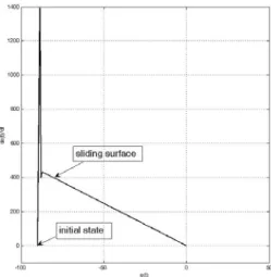
Figure 7 shows the simulation results of the control input signal u . The result in Fig. 8 shows that the system slides with minimum chattering. The simulation results verify that the proposed SMC controller can solve the problem that a conventional SMC cannot overcome when both the system functions and the bound of the disturbance signal are unknown. Additionally, the results verify that the SMC controller improves output chattering.
Fig.7 Simulation result of the control signal u.
Fig.8 Simulation result of sliding using proposed SMC
controller.
4. Experimental equipment and results
A manual SMAW process involves three steps: arc-starting, arcing, and arc-closing. The process begins with the electrode making instantaneous contact with the workpiece, and then being quickly pulled 2~4 mm up from the workpiece, leaving a bright arc between the end of the electrode and the workpiece. This step is called arc-starting. After the arc is initiated, the melting electrode starts to generate a molten pool on the workpiece. The step is called arcing during which the back and forth moving of the electrode in the perpendicular direction to the workpiece is controlled to maintain a fixed arc length, while the electrode is simultaneously moved along the welding path at a constant rate. At the end of welding path, waiting for some while before the arc hole being filled in, the electrode is quickly pulled up until the arc goes out. This step is called arc-closing. After this step, the molten pool cools down and freeze into a welded run that connects two workpieces. There will be some slag
covering on the welded run after the flux is melted. The welding process is completed by removing the slag.
The automatic welding process is similar to its manual operation. During the welding process, the step of arcing plays an important key in that the stability of the arc length is prone to vary from external disturbances to system uncertainties, affecting the final welding quality. It is suggested that a constant sensing and control on the arc current and the back and forth moving rate of the electrode be necessary to provide a stable arcing during the welding process [13]. Fig. 9 shows the experiment set-up of the SMAW system. A Hall-Effect type of current sensor is used to measure the arc current. Analog arc current is converted into digital signals by an A/D interface in the computer, where the proper control force, computed by the proposed controller, is converted to analog control signals by a D/A interface and then fed in the servo motor to control the feed-rate of the electrode. The developed SMAW system forms a closed-loop control system that can maintain not only a stable arc current but also a fixed arc length.
Before the welding experiment is performed, both the electrode and workpiece are not processed with rust-removing, wash-cleaning, and drying processes. The purpose is to introduce some unknown disturbance in the welding process. A SMAW machine with no system identification is used in the welding experiment, as shown in Fig. 10. During the experimental process, the E4313-type of electrode with diameter of 2.6 mm is moving along the welding path at a constant rate of 1mm/sec, and the back and forth moving rate of the electrode is controlled by the computer to ensure a stable arc current that maintains a fixed gap between the electrode and the workpiece.
Fig.9 Experiment set-up of the automatic SMAW system.
Fig.10 An automatic SMAW system without system
identification.
The control goal is that the system output current should be able to track the 100 amp. of arc current at the error convergence rate of e5t. Figure 11 shows the result of the arc current, where arc current xp is represented as thin solid line and the desired signal
d
x is represented as thick solid line. The result shows that the arc current is stable with minimum error. Figure 12 shows the result of the control input signal u .
Fig.11 The experimental result of arc current during the
arcing step.
Figure 12 shows the control input signal u . The experimental results verify that the proposed SMC, under the circumstances of no system identification, performs well in the error convergence and is effective in reducing chattering, which is a common problem in the conventional SMC. 15 20 25 -5 0 5 time c o nt ro l i n pu t
Fig.12 The control input signal u during the arcing step.
As shown in Fig. 13, the welding run on the low-carbon steel plate is of a fine ripple with same height, width, and interval.
Fig.13 Welding result of the automatic SMAW system.
Figure 14 and Fig. 15 show the result of arc current and the photograph of manual welding operation. As shown in Fig. 14, the arc current is far from stable. In Fig. 15, the welding run is somewhere narrow and high and somewhere wide and low, and the melt-drips spatter. It is clear that the results of automatic operation, either on arc current stability or on welding run homogeneity, are much better than that of manual operation.
25 30 35 0 20 40 60 80 100 120 time a rc cu rr e n t
Fig.14 Arc current output of manual welding operation.
Fig.15 Photograph of manual welding operation
5. Conclusions
This study focuses on the SMAW, a widely-used welding process by the industry, and develops an automatic SMAW control system. Simulation and experimental results show that the developed system can maintain a stable arc current and arc length to achieve superior welding quality than does a manual welding operation. Some main contributions of the proposed control system are described as follows:
(1) The capability of real-time measurement and control during welding process makes it easy to estimate working hours and costs, thereby improving welding production and quality while reducing costs.
(2) The automatic welding operation, as opposed to the manual operation, keeps operators far from the welding places, avoiding hazards, such as high-temperature, radiation, burning, and inhaling of toxic metal-chemical smoke, and increasing safety. It is worth to promote the use of automatic welding operation in many applications.
(3) The use of the function estimator, once the unknown function is estimated, help lower the piece-wise control force of the SMC control law and reduce chattering.
(4) When a finite-term Fourier series is used to approximate to any bounded function, some minor errors in the estimation, F~, g~, and Ted
~
may always exist. This kind of error, if existing on the system output, can lead to a minor error in the system or a problem that the control force is insufficient. This study solves this problem by introducing the term sgn(s) where the constant only requires being a small positive number while maintaining the same robustness in error estimation.
In summary, it is clear that a SMAW system is one of the non-deterministic, nonlinear systems. If a SMAW system is controlled by only linear techniques, it is possible that the performance requirements of global region operations will not be met. To improve welding performance, this study applies non-linear control theory on the SMAW process. The authors hope that, through this study, more advanced techniques, such as
intelligent control, image analysis, and robot automation, will be used in the research of SMAW process, facilitating the development of computerized mathematical applications.
Reference
[1] D. Smith, Welding skills and technology, McGraw-Hill, Boston, 1989.
[2] B. C. Howard Modern welding technology, Prentice-Hall, Englewood Cliffs, NJ, 1979.
[3] Leonard Koellhoffer, Shielded Metal Arc Welding, Wiley, 1983.
[4] Thomsen, J. S., Feedback Linearization based Arc Length Control for gas Metal Arc Welding, Proc. Of the American Control Conference (2005) 3568-3573.
[5] I. Tomashchuk, P. Sallamand, J.M. Jouvard, The modeling of dissimilar welding of immiscible materials by using a phase field method, Applied Mathematics and Computation, In Press, Corrected Proof, Available online 22 February 2012.
[6] R. B. Potts, X. -H. Yu, Difference equation modelling of a variable structure system , Computers & Mathematics with Applications, Volume 28, Issues 1-3, August (1994) 281-289.
[7] Yung-Ching Hung, Teh-Lu Liao, Jun-Juh Yan, Adaptive variable structure control for chaos suppression of unified chaotic systems, Applied Mathematics and Computation, Volume 209, Issue 2, 15 March (2009) 391-398.
[8] Chih-Jer Lin, Shyi-Kae Yang, Her-Terng Yau, Chaos suppression control of a coronary artery system with uncertainties by using variable structure control , Computers & Mathematics with Applications, Volume 28, Issues 1-3, August (1994) 281-289.
[9] K. K. Shyu, Y. W. Tsai and C. F. Yung, A Modified Variable Structure Controller. Automatica, Volume 28, Issue 6, November (1992) 1209-1213.
[10] J.-X. Xu, T.H. Lee, M. Wang and X. -H. Yu, Design of Variable Structure Controllers with Continuous Switching Control, International Journal of Control, Vol. 65 (1996) 409-431.
[11] Xiaobing Zhou, Yue Wu, Yi. Li, Hongquan Xue, Adaptive control and synchronization of a novel hyperchaotic system with uncertain parameters, Applied Mathematics and
Computation, Volume 203, Issue 1, 1 September (2008) 80-85.
[12] Mohammad Pourmahmood Aghababa, Mohammad Esmaeel Akbari, A chattering-free robust adaptive sliding mode controller for synchronization of two different chaotic systems with unknown uncertainties and external disturbances, Applied Mathematics and Computation, Volume 218, Issue 9, 1 January (2012) 5757-5768.
[13] Chien-Yi Lee, Pi-Cheng Tung and Wen-Hou Chu, Adaptive fuzzy sliding mode control for an automatic arc welding system, The International Journal of Advanced Manufacturing Technology Vol. 29, No. 5-6 (2006) 481-489.
[14] A.C. Huang and Y.S. Kuo, Sliding Control of Nonlinear Systems Containing Time-Varying Uncertainties with Unknown Bounds, International Journal of Control, Vol.74, No. 3 (2001) 252-264.
[15] W. Rudin, Principles of Mathematical analysis, McGraw-Hill, Inc., New York, 1976.